Efficient Estimation of $k$ for the Nearest Neighbors Class of Methods
- unpublished work from 2011 -

Abstract

The k Nearest Neighbors (kNN) method has received much attention in the past decades, where some theoretical bounds on its performance were identified and where practical optimizations were proposed for making it work fairly well in high dimensional spaces and on large datasets. From countless experiments of the past it became widely accepted that the value of $k$ has a significant impact on the performance of this method. However, the efficient optimization of this parameter has not received so much attention in literature. Today, the most common approach is to cross-validate or bootstrap this value for all values in question. This approach forces distances to be recomputed many times, even if efficient methods are used. Hence, estimating the optimal $k$ can become expensive even on modern systems. Frequently, this circumstance leads to a sparse manual search of $k$. In this paper we want to point out that a systematic and thorough estimation of the parameter $k$ can be performed efficiently. The discussed approach relies on large matrices, but we want to argue, that in practice a higher space complexity is often much less of a problem than repetitive distance computations.

1 Introduction

Since the introduction of the k Nearest Neighbor (kNN) method by Fix and Hodges in 1951 [1] a lot of different variants of it have appeared in order to make it suitable to different scenarios. The most notable improvements were done in terms of adaptive distance metrics [2][3][4], fast access via space partitioning (packed R* trees [5], kd-trees[6], X-trees[7], SPY-TEC [8]), knowledge base (prototype) pruning ([9],[10]) or classification based on sensitive distributed data ([13],[14],[15]). An overview over the state-of-the-art in nearest neighbor techniques is given in [11].

The continuing richness of investigation work into nearest neighbor can be explained with the omnipresence of CBR (Case Based Reasoning) type of problems [12] or just from the practical point of view of its massive parallelizability or simply populartiy. After all nearest neighbor is conceptually easy to understand - many students get to learn the nearest neighbor as the first classifier.

All of the beforehand mentioned advances evolve around the question of how to optimize the kNN’s distance measure for retrieving. The method’s apparent laziness might be the reason why a fast preoptimization of $k$ has not been paid a lot attention to.

The proper choice of $k$ is an important factor for achieving maximum performance of a kNN. However, as we will show, conventional $k$ optimization via cross-validation or bootstrapping is slow and promises potential for being sped up. Therefore, we will devote this paper to the concept of fast $k$ optimization.

There is work addressing this issue in an alternative way by introducing incremental kNN classifiers based on different types of trees. This class of nearest neighbors attempts to eliminate the influence of k by choosing the right $k$ ad hoc. The rationale behind this method is that for classification tasks the exact majority of a specific class label is not necessarily interesting. It is only interesting when nearest neighbor is used as a density estimator. In other cases it is generally enough to feel safe about which class label rules the nearest set. This class of nearest neighbor starts by polling a minimal amount of nearest neighbors. Then it analyzes the labels and if the retrieved collection of labels is indecisive it will poll more nearest neighbors until it considers the collection decisive enough.

Naturally, the method does not scale to small values of $k$, because e.g. a $k=1$ will never be indecisive. This is a problem because we know from experiments that small $k$ are often optimal. Incremental nearest neighbors have their strength in very large databases where typical queries do not need to compute all relative distances. During a lifetime of a large database some distances might not be computed at all. The lazy distance computation make incremental nearest neighbor methods ideal candidates for real time tasks operating on large volatile data. However, in a cross validation setup which needs to compute all distances incremental kNNs cannot play out their strengths. Because of the restrictions and intended use we exempted incremental methods from investigation in this paper.

We organize this paper in three parts. In the first part we will study the options to make the estimation of $k$ as fast as possible, in the second part we will experimentally compare the result with the conventional approach and in the last part we will draw a conclusion.

2 Stating the Problem

The kNN is commonly considered a classifier from the area of supervised learning theory. In this theory there exists a training function $T$ that delivers a model $m$ based on a set of options $o$, a matrix of example values $V$ and a vector of labels $l$ of respective size ($m=T(o,V,l)$). In turn, the model $m$ is used in a classification function $C$ that is presented with a matrix of new examples $V^{\prime}$ and its task is to deliver a vector of new labels $l^{\prime}$ ($l^{\prime}=C(m,V^{\prime})$). $T$ and $C$ must be related but there is no restriction on what the model can be. It can be a set of complex items, a matrix, a vector or just a single value, indeed.

From the perspective of a human the purpose of a model is to make predictions about the future. In order to be able to do this the human brain requires a simplification of the world. Only with the simplification of the world to a reduced number of variables and rules it can compute future states faster than they occur. In case of kNN the model $m$ consists of the data and of the smoothing parameter $k$. This means, that the function $T$ is an identity function between model and parameters. This conflicts with the common notion of a model because the production of models commonly implies reduction. However, the collected data already are a reduction of the world! From a practical point of view they can be considered as representative model states of the world and the data in the model is used to predict the class variable of a new vector before it is actually recorded. This fits perfectly well with the original notion of models. However, the model is only fixed, when $k$ is fixed.

According to the framework, fixing the model (getting the right value for $k$) is the job of the function $T$. Many training techniques in machine learning use optimization strategies developed for real numbers and open parameter spaces. This is not suitable for $k$ as it is an integer value and has known left and right limits: an ideal candidate for full search.

Most frameworks for pattern recognition offer macro optimization for the remaing model parameters that express themself in the initial training options $o$. The structural compatibility of the kNN with the pattern recognition frameworks’ macro optimization functions seduces the users very often to macro optimize $k$. The consequence of this is that kNN must compute distances repetitively as it cannot assume that specific vectors will simply exchange their role between training and testing in the future. In case of kNN this is exceptionally regrettable.

What does macro optimization mean for the computational complexity? Here we assume - but without loose of generality - that the dataset $V$ is of size $n$ ($n$-rows in matrix $V$) and can be exactly divided into $f$ equally sized partitions ready to be rearranged into $f$ different train and test setups. Since everything is being recomputed the computational complexity for this kind of cross-validation of $k$ for a brute kNN is $O\left(\hat{k}\cdot\frac{f-1}{f}\cdot n^{2}\right)$. $\hat{k}$ is the size of the tested range of $k$ and since we are considering full search we accept that $\hat{k}$ depends on the size $n$ of the dataset and the number of folds $f$. This means that the $\hat{k}=n\cdot\frac{f-1}{f}$. The scan of nearest sets yields a partial complexity of $O(\frac{f-1}{f}\cdot n^{2})$. Hence, for full search the total complexity is $O\left(\left(\frac{f-1}{f}\right)^{2}\cdot n^{3}+\frac{f-1}{f}\cdot n^{2}\right)$.

In order to reduce this high complexity it is necessary to optimize kNN within the train function $T$ as it has all necessary information about the relationships among the examples and the labels. This means that $T(o=\{k\},V,l)$ should become $T(o=\{i\},V,l)$ where $i$ is a vector of partition indices of the kind $(0,0,0,...,1,1,1,...,f,f,f...)^{T}$.

Now, the train function $T$ can utilize the fact that no new data will arrive during the training and all possible distance requests can be computed in advance. Distances within the same partition need not be computed as they will be never requested. These fields can be set to infinity (alternatively they can be filled up with the largest value found in the matrix + 1). The lower triangle is symmetrical to the upper triangle of the matrix because vectors between two points have the same norm. The distance matrix $D$ has a structure as shown in figure 1. The size of $D$ is $n\times n\times 2$. By $D(column,row)_{1}$ we mean the component distance and by $D(column,row)_{2}$ we mean the associated label.

Alone this redesign causes the complexity of the distance computations to get reduced to $O\left(\frac{f-1}{f}\cdot\frac{n^{2}}{2}\right)$. However this benefit is achieved at the expense of higher memory use. The brute kNN has a space complexity of $O(n)$, now the space complexity has risen to $O(n^{2})$.

The next step is to sort the vectors horizontally according to their distance. Although collecting the $k$ best solutions would be faster for a single run it means for a range of $k$ that you effectively obtain the insertion sort. Since there exist faster sorting algorithms we choose to sort but by using a different algorithm.

The fastest algorithm for doing so is the quick sort. Its average complexity is $O\left(n\log(n)\right)$. In the worst case scenario the sorting complexity of this method is $O\left(n^{2}\right)$. In that case $n$ rows will be sorted with $O\left(n^{2}\right)$. This means that the worst time complexity so far is $O\left(\frac{f-1}{f}\cdot\frac{n^{2}}{2}+n^{3}\right)$ and average case is $O\left(\frac{f-1}{f}\cdot\frac{n^{2}}{2}+n^{2}\log(n)\right)$.

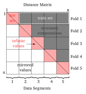
(a) Distance matrix and its computation requiring segments for the cross validation of $k$

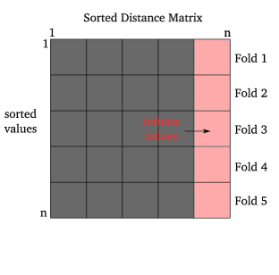
(b) Sorted distance matrix. Values are being sorted big values to the right

Figure 1: The distance matrix consists of tuples of data and label ($(d,l)$). It can be sorted horizontally without loosing the relationship between vector pair and ground truth.

In order to obtain nearest neighbors for each vector indexed by the row a counting matrix $M:=\mathbb{N}^{n\times s}$ is initialized with zeros. $s$ is the number of symbols or classes. For each row in $D$ and $M$ and for the columns $k=1..\frac{f-1}{f}n$ in $D$ the counters for the specific class label is increased. More precisely, for every row $r=1..n$ and for every tested $k$ the counters $M\left(D(k,r)_{2},r\right)$ are updated by $1$. The complexity of this operation is $O\left(\frac{f-1}{f}\cdot n^{2}\right)$. For the overall method this adds up to $O\left(\frac{3}{2}\frac{f-1}{f}\cdot n^{2}\right)$. In parallel the level of correct classification must be computed because after every modification of $M$ the state for the smaller $k$ is lost. Therefore a matrix $A:=\mathbb{N}^{\frac{f-1}{f}n\times f}$ for recording the number of correct classfications is required.

How is this number computed? At every round $k$ of the nearest neighbor candidate computations $M_{k}$ contains in each of its rows a vector that tells how many labels of specific kind are in the nearest neighbors set. The classification label is $l_{rk}^{\prime}=\underset{s}{\operatorname{argmax}}\hskip 2.84544ptM_{kr}$. The complexity for this operation is $O(n^{2}s)$.

This simple method is ambiguous by nature, as there can be many labels that are represented by the same amount of vectors in a nearby set. Computer implementations prefer to return the symbol with the smalest coding. However, it is possible to have a shadow matrix $S:=\mathbb{R}^{n\times s}$ that is the sum of the distances observed for each class label in the set so far. The rule for computing $S$ is the same as for $M$ with the difference that instead of adding ones to the matrix you add distances. When symbol frequency is ambiguous (argmax returns more than one value) it is possible to use $S$ to find which samples are closer overall. Because of the specific interest into fast $k$ optimization the simple argmax processing is used.

Now, every $l_{rk}^{\prime}$ is compared for equality with $l_{r}$ (ground truth) and the binary result is added to $A(k,i_{r})$. The $\underset{k}{\operatorname{argmax}}\hskip 2.84544ptA_{f}$ will return $f$ best $k$. $k^{*}$ is obtained by averaging.

Considering all parts of the algorithm together the overall complexity is $O\left(\frac{3}{2}\frac{f-1}{f}\cdot n^{2}+n^{2}\log(n)+n^{2}s\right)\approx O\left(n^{2}\log(n)\right)$

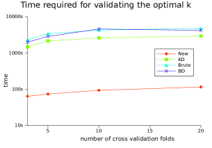
(a)

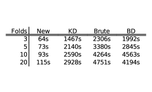
(b)

Figure 2: Experimentally established relationship between the number of folds and the algorithm speed.

3 Experiments

The method for fast $k$ computation (AutokNN) was tested against three other algorithms from the ANN library 1.1[16]: brute, kd-tree and bd-tree kNN with default settings. The AutokNN and its competitors performed a complete cross validation run on the ad, diabetes, gene, glass, heart, heartc, horse, ionosphere, iris, mushrooms, soybean, STATLOG australian, STATLOG german, STATLOG heart, STATLOG SAT, STATLOG segment STATLOG shuttle, STATLOG vehicle, thyroid, waveform and wine datasets with 3, 5, 10 and 20 folds. The goal of the experiment was the measurement of the time required to complete the full course of testing different $k$.

The data was separated into stratified partitions which were used in different configurations in order to obtain a training and a testing set. The AutoKNN computes the classification results for all $k$ while the other algorithms are bound to use a logarithmic search. By logarithmic search the following schema is meant: $k\in\{1,2,3,4,5,6,7,8,10,100,200,...,1000,...,\frac{f-1}{f}n\}$. This schema is practically motivated and rational under the assumption that the influence of additional labels on the result diminishes with higher values of $k$. Practical consideration is primarily test time. Example: while AutokNN required 15,35s for a complete scan based on the ad dataset, on same data exact brute kNN needed 353,7s in logarithmic mode and 19595,7s in full mode. The use of the logarithmic mode makes results with exactly the same values impossible. However, the differences in resulting $k$ and thus in accuracy were absolutely negligible so that the results are directly comparable nonetheless.

We added the experiment times for all databases up to a total for each cross validation size. The results are shown in the figure and the table under 2.

Time measurements were performed on a AMD Phenom II 965 with 8GB of RAM with a Linux 2.6.35 kernel. The algorithms are implemented in C/C++ and were compiled with gcc 4.4.5 with O3 option. Only core algorithm operation was measured and all time for additional I/O was ignored. For best comparability, ANN library sources were statically included.

4 Discussion and Conclusion

The Nearest Neighbor approach is considered user friendly and is frequently used for data mining, classification and regression tasks. It is embedded into many automatic environments that make use of kNN’s flexibility. Although kNN has been used, analyzed and advanced for almost six decades a repeating question can not be answered by current literature: What is the fastest way to estimate the right value for $k$ and what are the expenses for doing so.

The approach chosen here is to move the $k$ esimation away from the meta framework right into the training function $T$. The advantage of this is that additional information about the data can be made. This additional information allows to precompute the distances among all vectors without waste and to reuse them numerous times. From this design change which is known to practitioners but not discussed in literature a reduction in time complexity can be observed from $O\left(\left(\frac{f-1}{f}\right)^{2}\cdot n^{3}+\frac{f-1}{f}\cdot n^{2}\right)$ to $O\left(\frac{3}{2}\frac{f-1}{f}\cdot n^{2}+n^{2}\log(n)+n^{2}s\right)$ in average case. The experiments show, that this has significant impact on the speed of the $k$ estimation task. The comparison between kd-tree kNN and the proposed approach proves moreover that having a better time complexity saves practically more time than an efficient distance measure for this task.

The cost of this improvement is a higher space complexity (now $O(n^{2})$). In order to esimtate the practical impact of this complexity exchange we studied the contents of the UCI repository [17]. The UCI should be a reasonable crossover of the problems people face in real life.

Out of 162 datasets we found that 90% of them have less than 50K examples, 80% of them have less than 10K examples and half of the UCI’s datasets has less than 1000 examples (for exact distribution see Fig. 3). These sizes can be easily handled on higher class commodity computers.

This leads to the conclusion that turning in space complexity for time complexity is a good choice most of the time. Future implementations should offer an integrated $k$ searching. The results also show that the so found values for $k$ can be transfered not only to other exact kNN but also to approximate kNN working on kd-tree and bd-tree models.

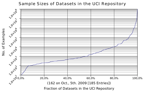
Figure 3: Dataset sizes in the UCI repository

5 Acknowledgments

This work has been made possible through the funding of the PaREn (Pattern Recognition and Engineering [18]) project by the BMBF (Federal Ministry of Education and Research, Germany).

APPENDIX

Appendix 0.A Influence of $k$ on the kNN Performance

The following diagrams are results from kNN based on natural and synthetic datasets. Synthetic datasets were obtained using WGKS [19] The standard deviation was estimated based on a 10x cross-validation. The diagrams are non linear. Sections of little change are compressed, hence x-axis are discontinuous.

See pages - of all_diagrams

References

- [1] Fix, E., Hodges, J.L. Discriminatory analysis, nonparametric discrimination: Consistency properties. Technical Report 4, USAF School of Aviation Medicine, Randolph Field, Texas, 1951.
- [2] Carlotta Domeniconi, Dimitrios Gunopulos, Jing Peng. Adaptive Metric nearest Neighbor Classification. CVPR, Vol. 1, pp.1517 (2000)
- [3] Jing Peng, Douglas R. Heisterkamp, H. K. Dai. Adaptive Kernel Metric Nearest Neighbor Classification. ICPR, Vol. 3, pp.30033 (2002)
- [4] T. Deselaers, R. Paredes, E. Vidal, H. Ney. Learning Weighted Distances for Relevance Feedback in Image Retrieval. ICPR 2008, Tampa, Florida, USA (08/12/2008)
- [5] I. Kamel, C. Faloutsos. On Packing R-trees. Proceedings of the 2nd Conference on Information and Knowledge Management (CIKM), Washington DC (1993)
- [6] Thomas H. Cormen, Charles E. Leiserson, Ronald L. Rivest. Introduction to Algorithms. ch. 10, MIT Press and McGraw-Hill (2009)
- [7] S. Berchtold, D. Keim, H.-P. Kriegel. The X-tree: An index structure for high-dimensional data. In Proceedings of 22th International Conference on Very Large Databases (VLDB’96), pp 28–39, Morgan Kaufmann (1996)
- [8] Dong-Ho Lee, Hyoung-Joo Kim. An Efficient Technique for Nearest-Neighbor Query Processing on the SPY-TEC. IEEE Transactions on Knowledge and Data Engineering, Vol. 15, No. 6, pp. 1472-1486, IEEE Educational Activities Department,Piscataway, NJ, USA (2003)
- [9] Jose Salvador-Sanchez, Filiberto Pla, Francesco J. Ferri. Prototype Selection for the Nearest-Neighbor Rule Through Proximity Graphs. PRL, Vol. 18, No. 6, pp. 507-513 (1997)
- [10] U. Lipowezky. Selection of the optimal prototype subset for 1-NN classification PRL, Vol. 19, No. 10, pp. 907-918 (1998)
- [11] Keith Price Bibliography - Nearest Neighbor Literature Overview http://www.visionbib.com/bibliography/pattern622.html
- [12] David W. Aha. The Omnipresence of Case-Based Reasoning in Science and Application. Journal on Knowledge-Based Systems, Vol 11, pp. 261-273 (1998)
- [13] Young, B., Bhatnagar, R.: Secure K-NN Algorithm for Distributed Databases. University of Cincinnati (2006)
- [14] Shaneck, M., Yongdae, K., Kumar, V.: Privacy Preserving Nearest Neighbor Search. Dept. of Computer Science Minneapolis (2006)
- [15] Kantarcıoglu, M., Clifton, C.: Privately Computing a Distributed -nn Classifier. LNCS, Vol. 3202, 279–290 (2004)
- [16] Mount, D. M.: Approximate Nearest Neighbor Library 1.1, Department of Computer Science and Institute for Advanced Computer Studies, University of Maryland (2010)
- [17] UCI Machine Learning Repository: http://archive.ics.uci.edu/ml
- [18] Pattern Recognition and Engineering (PaREn), DFKI, BMBF Project: http://paren.iupr.com/ (2008 - 2010)
- [19] Janick V. Frasch and Aleksander Lodwich and Faisal Shafait and Thomas M. Breuel A Bayes-true data generator for evaluation of supervised and unsupervised learning methods. Pattern Recognition Letters, volume 32:11, p.1523-1531, 2011, doi: 10.1016/j.patrec.2011.04.010