Modulated phases in external fields: when is reentrant behavior to be expected?

Abstract

We introduce a new coarse grain model capable of describing the phase behavior of two dimensional ferromagnetic systems with competing exchange and dipolar interactions, as well as an external magnetic field. An improved expression for the mean field entropic contribution allows to compute the phase diagram in the whole temperature versus external field plane. We find that the topology of the phase diagram may be qualitatively different depending on the ratio between the strength of the competing interactions. In the regime relevant for ultrathin ferromagnetic films with perpendicular anisotropy we confirm the presence of inverse symmetry breaking from a modulated phase to a homogenous one as the temperature is lowered at constant magnetic field, as reported in experiments. For other values of the competing interactions we show that reentrance may be absent. Comparing thermodynamic quantities in both cases, as well as the evolution of magnetization profiles in the modulated phases, we conclude that the reentrant behavior is a consequence of the suppression of domain wall degrees of freedom at low temperatures at constant fields.

I Introduction

The field versus temperature phase diagram of ultra-thin ferromagnetic films displaying stripe, bubbles and homogeneous phases has attracted attention in recent years, mainly due to the existence of new experimental results from which the phase diagram and other interesting characteristics of the phase transitions have been reported Saratz et al. (2010a, b). Early theoretical results on the phase diagram from an effective model with dipolar interactions were challenged Garel and Doniach (1982) by experiments. The main qualitative difference between early phase diagrams and recent experimental results was the observation of an inverse symmetry breaking (ISB) transition, with a sequence of homogeneous-modulated-homogeneous phases, as the temperature is lowered at fixed external field Saratz et al. (2010a, b). The existence of an ISB transition in such systems had been predicted in the pioneer work of Abanov et alAbanov et al. (1995), using a phenomenological approach. Subsequent theoretical work analyzed the existence of ISB from a scaling hypothesis Portmann et al. (2010); Mendoza-Coto and Stariolo (2012). Reentrant behavior was shown on a coarse-grained model of the Landau-Ginzburg type Cannas et al. (2011), although no attempt was made to explain the nature of the reentrance, mainly due to limitations in the very definition of the model, which was not able to capture the low temperature sector of the phase diagram. Recently, Velasque et. al. studied a mean field version of the dipolar frustrated Ising ferromagnet (DFIF), and showed that the stripe phase in a field presents reentrant behavior Velasque et al. (2014). Furthermore, by comparing the DFIF with two simpler models, the authors concluded that the reentrant behavior in this kind of systems has its origin on the entropy gain from domain walls degrees of freedom of modulated structures.

Inverse freezing in magnetic models has been observed mainly in spin glasses and disordered systems, in which frustration leads to complex entropic contributions Sellitto (2006); Paoluzzi et al. (2010); Silva et al. (2012); Erichsen et al. (2013). Nevertheless, the question of the physical origin of reentrant behavior remains obscured by the inherent complexity of the thermodynamic behavior of disordered systems. Magnetically frustrated systems without quenched disorder, where low temperature phases and ground states display known symmetries, seem to be better candidates for getting a better understanding of ISB Portmann et al. (2010); Cannas et al. (2011); Velasque et al. (2014). Besides ultrathin ferromagnetic systems with dipolar frustration, other frustrated systems without quenched disorder showing inverse transitions are, e.g. the $J_{1}$-$J_{2}$ model in the square lattice Yin and Landau (2009); de Queiroz (2011) and the axial next-nearest-neighbor Ising (ANNNI) model Yokoi et al. (1981).

The aim of the present work is twofold: first, we introduce a new coarse-grain model for ultrathin ferromagnetic films with perpendicular anisotropy which, at variance with previous ones, is valid at any temperature, allowing the computation of the complete phase diagram. By minimizing the corresponding free energy in a mean field approximation, we obtain the magnetic field versus temperature phase diagram showing homogeneous paramagnetic, stripes and bubbles phases. This spans the complete phenomenology observed in experiments Saratz et al. (2010a, b). Furthermore, we show that in the experimentally relevant sector of coupling constants the system shows inverse symmetry breaking, but for general values of the ratio between the competing interactions, this is not always the case. Thus, we concentrate our discussions on two relevant cases, one showing ISB and another without reentrance, and analyze the origin of the different behaviors between them. Second, we discuss the physical origins of inverse symmetry breaking in this kind of systems. We present compelling evidence that the inverse transition is driven by the excess of degrees of freedom present in the domain walls, namely, a basically entropy-driven mechanism. We show that the domain wall structure and evolution with temperature and magnetic field is very different in the two prototypical cases studied, which reinforces the argument on the relevance of domain wall structure for ISB, complementing and expanding the analysis of reference Velasque et al., 2014.

The organization of the paper is as follows: in Section II we introduce the model and the mean field approximation. In III we present the results for the magnetic field versus temperature phase diagrams and analyze the nature of the reentrant behavior and the nature of the phase transitions observed. In Section IV we conclude with a summary of the results.

II Model

Modulated phases in ultrathin ferromagnetic films occur at mesoscopic scales, i.e. the typical length scale of the modulations in the magnetization density are much larger than the lattice spacing, thus justifying a coarse grained description (see, e.g. reference Portmann et al. (2010) for a detailed justification of the coarse grained description in this kind of systems). Then, our starting point is the effective hamiltonian:

$$H[\phi]=\frac{1}{2}\int d^{2}x\;\left(\vec{\nabla}\phi(\vec{x})\right)^{2}+\frac{1}{2}\iint d^{2}xd^{2}x^{\prime}\,J(|\vec{x}-\vec{x}^{\prime}|)\phi({\vec{x}})\phi({\vec{x}^{\prime}})-B\,\int d^{2}x\;\phi({\vec{x}}),$$ (1)

where $\phi({\vec{x}})$ is the out of plane magnetization density, the first term represents the effective short range exchange interaction, the second term is a competing long range dipolar interacion, which in the limit of strong perpendicular anisotropy reduces to the form $J(x)=J/x^{3}$ and the last one is a coupling to an external homogeneous magnetic field $B$ perpendicular to the plane of the film. Within a mean field approximation, we can then construct an effective free energy functional $F[\phi]=H[\phi]-T\,S[\phi]$, which after a minimization respect to the field $\phi$ gives us the equilibrium state ($S[\phi]$ being some properly defined entropy functional). Then, the effective free energy reads

$$F[\phi]=\frac{1}{2}\iint d^{2}xd^{2}x^{\prime}\,A(\left|{\vec{x}}-{\vec{x}}^{\prime}\right|)\phi({\vec{x}})\phi({\vec{x}^{\prime}})-\frac{1}{\beta}\int d^{2}x\;{\cal S}(\phi({\vec{x}})/\phi_{0})-B\,\int d^{2}x\;\phi({\vec{x}})$$ (2)

where ${\cal S}(x)$ is an entropy density, $\phi_{0}$ corresponds to the saturation value of the magnetization, $\beta=(k_{B}T)^{-1}$ and the quadratic kernel $A(\left|{\vec{x}}-{\vec{x}}^{\prime}\right|)$ encodes all the information about the physical interactions in the system. Note that, up to this point, the model defined is quite general. Previously considered coarse grained models have been mainly of the Ginzburg-Landau type, defined by an expansion in powers of the order parameter, typically up to $\phi^{4}$, which limits the validity of results to temperatures near the critical point Portmann et al. (2010); Cannas et al. (2011). Instead, in line with the mean field approximation, we consider an entropy density function to be of the form:

$${\cal S}(x)=\frac{1+x}{2}\log{\frac{1+x}{2}}+\frac{1-x}{2}\log{\frac{1-x}{2}}.$$ (3)

This form imposes saturation values to the order parameter $|\phi(\vec{x})|\leq\phi_{0}$ and allows a computation of the thermodynamic properties for any temperature.

It is well known that the solutions which minimize the effective free energy (2) (at low enough temperatures) correspond to periodic patterns in space in the form of stripes or bubbles Garel and Doniach (1982); Seul and Andelman (1995). The general solution for the order parameter can be written as a Fourier series expansion of the form $\phi(\vec{x})=\sum_{i=0}^{\infty}c_{i}\cos\left(\vec{k}_{i}\cdot\vec{x}\right)$. Different sets of wave vectors will define different patterns, so part of the problem is to choose the appropriate set of wave vectors for constructing the particular solutions expected. Replacing the general solution into Eq.(2), and after a Fourier transformation, the free energy density reads:

$$f[\phi]=\frac{F[\phi]}{V}=\frac{1}{2}\hat{A}(0)\,c_{0}^{2}+\frac{1}{4}\sum_{i}\hat{A}(k_{i})\,c_{i}^{2}-\frac{1}{\beta V}\int d^{2}x\;{\cal S}\left(\sum_{i}c_{i}\cos\left(\vec{k}_{i}\cdot\vec{x}\right)\right)-B\,c_{0},$$ (4)

where $V$ is the total volume (area) of the system. The function $\hat{A}(\vec{k})$ stands for the Fourier transform of $A(x)$ (fluctuation spectrum) and $c_{0}$ represents the amplitude of the zero wave vector mode. Since the function $A(x)$ is the sum of two competing interactions, it turns out that the Fourier transform of the model defined in (1) has a minimum at a nonzero wave vector $k_{0}$. This signals the fact that the competition between exchange and dipolar interactions favors the formation of periodic patterns in the order parameter. The value of $k_{0}$ corresponds to the optimum wave vector for the formation of single mode modulated structures and sets a natural characteristic length scale for the system. Hence, from now on, all wave vectors will be expressed in units of $k_{0}$ ($k_{0}=1$) and all lengths in units of $2\pi/k_{0}$.

It is also useful to express the energy in units of $|\hat{A}(k_{0})|$ and the temperature in units of $|\hat{A}(k_{0})|/k_{B}$, so that

$$f[\phi]=\frac{1}{2}{\cal A}(0)\,c_{0}^{2}+\frac{1}{4}\sum_{i}{\cal A}(k_{i})\,c_{i}^{2}-Ts-h\,c_{0},$$ (5)

where ${\cal A}(k)=\hat{A}(k)/|\hat{A}(k_{0})|$, $h=B/|\hat{A}(k_{0})|$ and $s$ is the entropy per volume unit. The expression above is written in terms of dimensionless variables only, which makes it suitable for numerical work.

In order to develop modulated patterns of typical scale $k_{0}$, $A(k)$ should have a negative minimum. Such condition ensures the necessary stability of those modes near the circumference of radius $k_{0}$, and consequently the formation of modulations in the order parameter. Consequently ${\cal A}(k_{0})=-1$. Considering that the short range part of $A(k)$ is proportional to $k^{2}$ in the long wavelength limit, and that in the same limit the dipolar interaction gives a contribution proportional to $-k$ Czech and Villain (1989); Pighín and Cannas (2007), the appropriate form for ${\cal A}$ for the systems considered here has the general form:

$${\cal A}(k)=-1+a(k-1)^{2}.$$ (6)

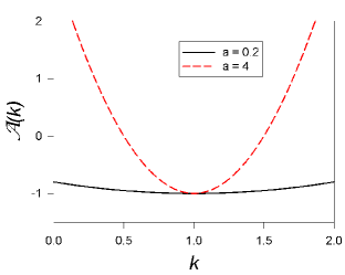
Figure 1: (Color online) The spectrum of fluctuations $A(k)$ of equation (6) for two values of the curvature parameter $a=0.2$ and $a=4$.

The only free parameter in the fluctuation spectrum (6) is the curvature $a$. In figure 1 the fluctuation spectrum is shown for two representative values of the parameter $a$. In the following it will be shown that these two cases have very different phase diagrams.

Regarding the ground states or low energy configurations of these kind of systems, to our knowledge, the only exact results available correspond to the ground states of the square lattice Ising model with ferromagnetic nearest neighbor interactions plus antiferromagnetic dipolar interactions proportional to $1/r^{3}$ Giuliani et al. (2006, 2011), where it has been shown that the ground states at zero external field are striped patterns for large enough ferromagnetic interactions, limit relevant to experimental ultrathin films with perpendicular anisotropy. For finite external fields there are no exact results but, based on experimental evidence of low temperature patterns, a series of interesting works have compared the energetics of striped, bubbles, checkerboard and homogeneous configurations Cape and Lehman (1971); Ng and Vanderbilt (1995); Saratz et al. (2010b). All the theoretical evidence indicates that, at zero temperature and low enough fields, the striped configurations have the lower energy, until a critical field value from where an hexagonal array of bubbles becomes the ground state. At still a higher critical field, the homogeneously magnetized state turns to be the lowest energy state. Then, the relevant equilibrium configurations of the density field $\phi(\vec{x})$ may be of two different types: striped configurations which can be written in the form:

$$\phi_{s}({\vec{x}})=\sum_{i=0}^{\infty}c_{i}\cos(k_{eq}\,\vec{s}_{i}\cdot{\vec{x}}),$$ (7)

with the vectors ${\vec{s}_{i}}=i(1,0)$, and bubble configurations:

$$\phi_{b}({\vec{x}})=\sum_{i=0}^{\infty}c_{i}\cos(k_{eq}\,{\vec{b}}_{i}\cdot{\vec{x}}),$$ (8)

where the set of vectors ${\vec{b}}_{i}$ are defined on a triangular lattice with lattice spacing equal to one. The details of the definitions of the wave vectors forming the bubbles solutions are shown in the Appendix. In both cases $k_{eq}$ represents the equilibrium wave vector that defines the modulation length for each structure. Substituting Eqs.(7) and (8) into Eq.(5) leads to a mean field variational free energy in terms of the infinite set of amplitudes $\{c_{n}\}$ and $k_{eq}$. After truncating Eqs.(7) and (8) to some maximum number of modes $n_{max}$, variational expressions at different levels of approximation for the stripes and bubbles free energies are obtained. Assuming that the only equilibrium states are stripes, bubbles or homogeneous ones, we determined the equilibrium phase diagram by minimizing and comparing the free energies for each type of solution to the same fixed level of approximation $n_{max}$. The functional minimization was performed by the method of Gaussian quadratures.

III Results

In figures 2 and 3 we show the magnetic field ($h$) versus temperature ($T$) phase diagrams for two representative cases: $a=4$ and $a=0.2$. As can be seen, the topology is very different in each case. In both cases, three thermodynamic phases can be possible: stripes, bubbles and uniform, qualitatively similar to observations in experiments. The value of $a$ determines whether the phase diagram will show reentrant behavior or not, both cases being possible. Comparing expression (6) with a more microscopic one, e.g. the spectrum of the dipolar frustrated Ising ferromagnet considered in Pighín and Cannas (2007); Velasque et al. (2014), it can be shown that $a\propto 1/\delta^{2}$, where $\delta=J/g$, $J$ being the strength of the short range exchange interaction and $g$ the intensity of the competing dipolar interaction. In the modulated sector of the dipolar frustrated Ising model, $\delta\gg 1$ and therefore $a$ takes typically a small value. We will see in the following that this leads to reentrant behavior, consistent with what is observed in experiments on ultrathin ferromagnetic films. Nevertheless, for small $\delta$, reentrant behavior is absent, as can be seen in the phase diagram of figure 2.

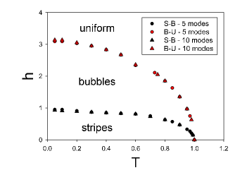
Figure 2: (Color online) External field versus temperature phase diagram for $a=4$ and different degree of approximations $n_{max}$.

As shown in the figure, in this case at low fixed temperature the model goes through two successive transitions as the external field is raised. At zero and low fields the stripe configurations are the equilibrium phase of the model Pighín and Cannas (2007); Cannas et al. (2011); Velasque et al. (2014), but at a critical field the magnetized background triggers an instability towards bubble solutions, which are the equilibrium ones at intermediate fields until a transition to a uniformly magnetized paramagnetic state takes place at a second critical field. As the field is raised the stripes develop a finite magnetization in the form of an asymmetry favoring the direction parallel to the field. This asymmetry grows and eventually leads to the bubble equilibrium phase. Both the asymmetry and modulation length grow with the field in a way similar to what was observed in the dipolar frustrated Ising model in Ref.[Velasque et al., 2014], and seems to diverge at the critical field where the homogenous phase sets in, as it will be discussed later. Remarkably, both transition lines become almost independent of $n_{max}$ for relatively small values of it ($n_{max}=5$) even at very small temperatures. This means that both modulated solutions present basically the same wall structure at all temperatures.

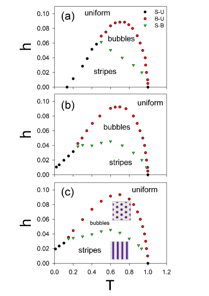
Figure 3: (Color online) External field versus temperature phase diagram for $a=0.2$. Different panels correspond to $n_{max}$ equal to (a) 5, (b) 10, (c) 15.

For small values of $a$, the $h-T$ pase diagram shows reentrant behavior. In figure 3 we show three instances of the phase diagram, depending on the maximum number of modes considered in the stripes and bubbles solutions given by equations (7) and (8). In the bottom panel we show two pictures illustrating the real space stripes and bubbles solutions. For the three cases considered, $n_{max}=5,\,10$ and $15$, the qualitative picture is the same. Nevertheless, it can be seen that the triple point, at which the three different phases meet, drifts to the left as $n_{max}$ grows. Then, it can be expected that, in the limit $n_{max}\to\infty$, this point will either be at $T=0$ or it will simply disappear. Computational limitations prevented us of reaching larger values of $n_{max}$, and then the solutions began to be unreliable at very low temperatures, where more and more modes acquire a finite weight in the variational profiles. This trend is in line with experimental results on the phase diagram for Fe/Cu(001) ultrathin films Saratz et al. (2010a, b).

To get some insight on the nature of the reentrant behavior we first look at the thermodynamic functions. Figure 4 shows the entropy and free energy versus temperature, for $a=0.2$ and fixed external field $h=0.06$, which goes through the bubbles phase for $n_{max}=15$ (see figure 3). The free energy crossing associated with both phase transitions (uniform to bubbles and bubbles to uniform as $T$ increases) appear clearly in Fig.4b. We see that both phase transitions result from a subtle balance of both the energy $E$ and the entropy $S$ ($f=E-TS$) as indicated by color codes in the figure. At temperatures $T<0.55$ both the energy (not shown) and the entropy of the bubbles phase are larger than the corresponding quantities in the uniform phase. At very low temperatures the influence of the energy is stronger than the influence of the entropy and the uniform phase is the stable one. At the ISB transition point ($T\approx 0.3$) such balance inverts and the bubbles phase becomes the stable one. Hence, the behavior of the entropy becomes crucial to the appearance of the ISB transition. On the other hand, at the direct transition from bubbles to uniform ($T\approx 0.9$) the roles played by energy and entropy are interchanged: the uniform phase has both larger entropy and energy than the bubbles. At the transition point the decrease in the internal energy of the uniform phase counterbalances the larger entropy of the bubbles. Consistently, the same behavior is observed in Fig.5 when $a=4$, in the non reentrant regime. In this case, the entropy of the uniform phase is larger than in the bubbles one at all temperatures, so the only relevant thermodynamical quantity is the energy, at least as far as the phase transition is concerned.

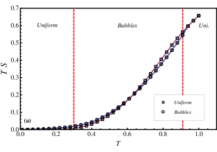
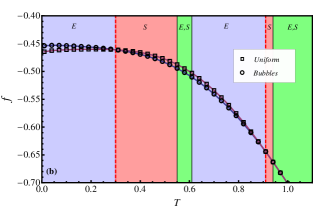
Figure 4: (Color online) Thermodynamic functions of the bubbles and uniform phases for $a=0.2$, $h=0.06$ and $n_{max}=15$. The dashed red lines mark the different transition temperatures for the present field. (a) $T\,S$ as a function of $T$. (b) Free energy as a function of $T$. The background colors indicate whether the free energy balance favors the stable phase as a result of having both smaller internal energy and larger entropy than the other (E,S), larger entropy only (S) or smaller energy only (E).

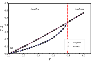
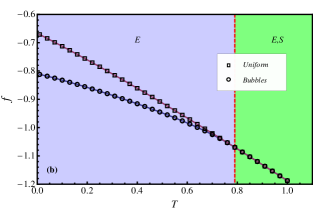
Figure 5: (Color online) Thermodynamic functions of the bubbles and uniform phases for $a=4$, $h=2$ and $n_{max}=15$. The dashed red lines mark the transition temperature for the present field(a) $T\,S$ as a function of $T$. (b) Free energy as a function of $T$. The background colors indicate whether the free energy balance favors the stable phase as a result of having both smaller internal energy and larger entropy than the other (E,S) or just smaller energy (E).

In reference [Velasque et al., 2014] it was suggested that the excess entropy of domain walls degrees of freedom was responsible for the reentrant behavior seen in the dipolar frustrated Ising model in the stripes phase. Here, we confirm that expectation. It is again instructive to compare the behavior of characteristic quantities for the cases with and without reentrance in our model. In figure 6 we show two dimensional cuts of the bubbles magnetization profiles in the two cases $a=4$ (top panel) and $a=0.2$ (bottom panel) at a fixed value of the magnetic field, characteristic in each phase diagram, and $n_{max}=15$. In each panel two profiles, corresponding to two characteristic temperatures, are shown. The temperatures were chosen to be near the high temperature transition and a sufficient low temperature in each case. It is possible to see that the profiles change little between both temperatures in the model without reentrance. The domain wall width is large, of the order of the modulation length $\lambda=2\pi/k_{eq}$, both at high and low $T$. On the contrary, in the model with ISB the profile changes qualitatively from high to low $T$. At high $T$ the profile is more sinusoidal; few modes have finite weight in the Fourier expansion. As the temperature is lowered more and more modes acquire a finite weight, and the profile evolves to a square wave-like one. At exactly zero temperature, the profile will be exactly a square wave, which has zero entropy. From the entropic contribution perspective, this means that while for the $a=4$ model the entropy contribution of domain walls is nearly the same in the whole temperature range, for the $a=0.2$ model the walls rapidly loose entropy as the temperature approaches low values. In the inset of the bottom panel in figure 6 we show the change in domain wall width relative to the modulation length. Our conclusion is that this important loss of entropy of domain walls is responsible for the inverse symmetry breaking phenomenon observed in ultrathin ferromagnetic films. Also note that, according to figure 1, for large values of the inverse curvature $a$, the low energy physics is dominated by a few modes around the minimum of Eq.(6). This is reflected in a weak temperature dependence of the modulation length and wall width, as shown in the top panel of figure 6. At variance with this behavior, for a large curvature (small $a$ values), the spectrum of fluctuations is shallow, implying that many modes can be accommodated with a moderate change in energy/temperature. This is again reflected in the bottom panel of figure 6, where a sharp change in the magnetization profiles of the bubbles phase is observed as the temperature is changed.

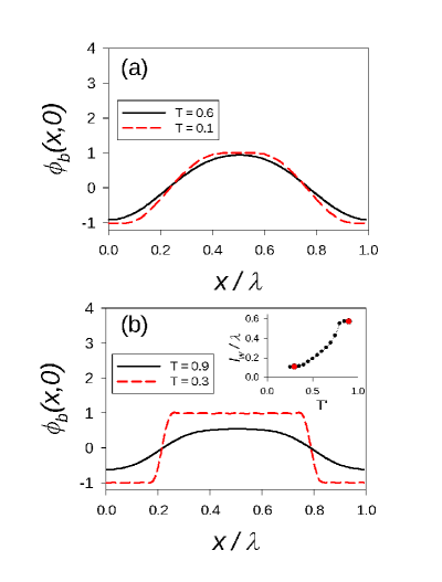
Figure 6: (Color online) Domain wall width behavior in the bubbles magnetization profiles for $n_{max}=15$. (a) Non reentrant region $a=4$ and $h=2$. (b) Reentrant region $a=0.2$ and $h=0.06$. The inset shows the domain wall width $l_{w}$ to wave length $\lambda$ ratio ($\lambda=2\pi/k_{eq}$) as a function of the temperature. Red circles mark the boundaries of the bubbles phase.

Another result of particular interest for the model is the nature of the transition from the bubbles phase to the homogeneous one at the critical field $h_{c}$. In figure 7 we show the evolution of the modulation length at fixed temperature $T=0.8$ as the critical field is approached from the bubbles phase for different values of $n_{max}$, in the $a=0.2$ model. The behavior for $a=4$ and other values of $T$ is qualitatively similar. Previous works suggested that the critical field lines correspond to first order phase transitions Cannas et al. (2011), with a discontinuous jump in the modulation length and magnetization. Nevertheless, as anticipated in an analysis of the stripes solutions for the dipolar frustrated Ising model Velasque et al. (2014), the transitions turn out to be continuous in the whole critical line when the limit of large number of modes is reached. Figure 7 shows, for $T=0.8$, that for any finite value of $n_{max}$ the modulation length $\lambda$ first grows as the field approaches the critical one, but eventually saturates at a finite value, suggesting a discontinuous jump at $h_{c}$. Nevertheless, the saturation value grows itself as $n_{max}$ grows. In order to get an estimation of the asymptotic behavior, we have fitted the data (shown in log-log scale) with hyperbolic functions. A scaling analysis of the saturation value of $\lambda$ (not shown) suggests that it diverges with the power law $(h_{c}-h)^{-0.4}$. The dashed line (in red) shows this asymptotic behavior, implying that, in the limit $n_{max}\to\infty$, the modulation length grows continuously as $h_{c}$ is approached and the homogeneous phase emerges as the limit $\lambda\to\infty$. A confirmation of the continuous character of the phase transition to the uniform phase comes from an analysis of the size of the jump in the magnetization at the critical field. In figure 8 we show the difference between the magnetizations of the homogeneous and bubbles ($m_{u}-m_{b}$) solutions at $T=0.8$ and $h_{c}$ versus $n_{max}$. A fit of the five points available in logarithmic scale shows that the jump goes to zero as $n_{max}\to\infty$ with a power law $n_{max}^{-1.56}$. Preliminary results indicate that the bubbles-paramagnetic transition is continuous in the whole critical line, determination of critical exponents along the line is left for future work.

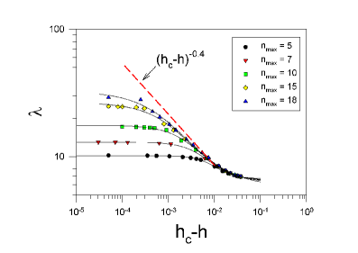
Figure 7: (Color online) Bubbles modulation wavelength $\lambda$ as the transition field $h_{c}$ is approached from the bubbles phase at fixed temperature $T=0.8$ and different values of $n_{max}$, in the $a=0.2$ model. The continuous lines are fittings using hyperbolic functions in the log-log scale.

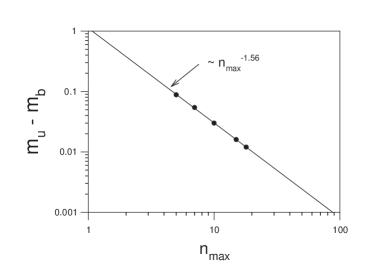
Figure 8: (Color online) Magnetization jump at the critical field between the bubbles and uniform phases for $T=0.8$ versus $n_{max}$ in log-log scale, in the $a=0.2$ model.

IV Conclusions

We introduced a coarse grained model for stripe forming systems (such as ultrathin magnetic films), that generalizes the usual Landau–Ginzburg one. The inclusion of a complete mean field entropic form (instead of its expansion) allowed us to obtain the $(h,T)$ phase diagram at any temperature, not only close to the critical one. The method is completed by proposing variational modulated solutions, namely bubbles and stripes, in the form of appropriately truncated Fourier expansions.

After an appropriated rescaling, the fluctuation spectrum of the model can be characterized by a single parameter, namely, the inverse curvature at the minimum of the spectrum, $a$. We found that $a$ determines the existence or not of ISB transition. For ultrathin magnetic films models, large values of $a$ mean small values of $\delta$, namely, the exchange to dipolar couplings ratio. We found that for large values of $a$ the phase diagram does not display ISB. This behavior is therefore consistent with previous Monte Carlo simulation results Cannas et al. (2011); Díaz-Méndez and Mulet (2010) for small values of $\delta$, where no ISB were observed.

For small enough values of $a$ the ISB transition emerges and the phase diagram displays (in the limit $n_{max}\to\infty$) the same topology observed experimentally in Fe on Cu filmsSaratz et al. (2010a, b). Moreover, when $a$ is small enough, an ISB transition is observed not only between the uniform and the bubbles solution, but also between stripes and bubbles for large enough values of $n_{max}$ (see Fig.3), an experimentally verified factSaratz et al. (2010a). Our results also show the presence of a triple point between bubbles, stripes and uniform phases for finite values of $n_{max}$. However, such point moves towards lower temperatures as $n_{max}$ increases suggesting that, in the $n_{max}\to\infty$ limit, either it is driven to $T=0$ or it simply disappears. In other words, it would be probably an spurious effect of the finite mode approximation. This last scenario would be consistent with the ground state calculations of Ref.[Saratz et al., 2010b]. On the other hand, our results appear to be consistent with the existence of a triple point between the three phases at $(T,h)=(T_{c},0)$, for any value of $a$, in the sense that, within our numerical resolution, both transition lines join at such point and are independent of $n_{max}$ in its neighborhood.

We observed a clear correlation between the appearance of the ISB transition and the low temperature domain wall behavior at the modulated phases. In the non reentrant regime, i.e. when $a$ is large, the magnetization profiles in the modulated phases exhibit extended domain walls whose width (relative to the modulation length) varies very little with the temperature, down to very low values of $T$. On the contrary, when the ISB transition is present the domain wall width shows a strong variation with temperature, becoming very sharp as the temperature decreases approaching the ISB. Such phenomenon is completely consistent with the phenomenological scaling hypothesis stated in Ref.[Portmann et al., 2010], according to which a change in the nature of the domain walls should be enough to explain the appearance of ISB. The change in magnetization profile is consistent with a shallow spectrum around its minimum (small values of $a$), since the system can accommodate a large number of modes (necessary condition to develop sharp domain walls) with a moderate change in energy/temperature. Finally, our results suggest that (at least at the mean field level) the whole transition line between the modulated and non modulated phases (i.e., bubbles and uniform) is continuous with continuously diverging wave length, consistently with the results of Ref.[Velasque et al., 2014].

IV.1 Construction of the bubbles solution

In this appendix we discuss in some detail how the bubbles solution is constructed and which are its features. In the kind of systems under study here, the bubble pattern is composed by a triangular regular array of circular bubbles, distributed over a background of homogeneous magnetization. The bubbles are magnetized contrary to the background in order to minimize the dipolar energy cost in the free energy functional.

From first principles we know that we can construct our bubble solution $\phi_{b}({\vec{x}})$ as a superposition of one dimensional modulations with the correct set of wave vectors. In this way we can write the solution in the form:

$$\phi_{b}({\vec{x}})=\sum_{i=0}^{\infty}c_{i}\cos(k_{eq}\,{\vec{b}}_{i}\cdot{\vec{x}}),$$ (9)

where the wave vectors $\{\vec{b}_{i}\}$ are selected as forming a triangular lattice with lattice size equal one. At the same time, since we have a regular array in which all bubbles are identical, we need to impose some conditions to the Fourier amplitudes of our solution. This condition implies that all those Fourier amplitudes corresponding to wave vectors $\vec{b}_{i}$’s related by symmetry operations of the triangular lattice are equal.

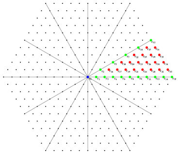
Figure 9: (Color online) Lattice of wave vectors for a bubbles pattern considering $n_{\mathrm{max}}=10$. Each dot represents a different wave vector $\vec{b}_{i}$ considered to build our solution.

In this way, once we have chosen the maximum number of modes in the principal directions $n_{\mathrm{max}}$, it is automatically defined how many independent Fourier amplitudes we need to consider. In Figure 9 we show the case of $n_{\mathrm{max}}=10$. For this particular choice, of the initial set of $331$ Fourier amplitudes corresponding to the set ${\vec{b}_{i}}$, after considering the symmetry arguments we are left with only $35$ independent components, as shown in Fig. 9 with bigger points. This reduction in the number of Fourier coefficients greatly simplifies the numerical work. Moreover, as can be observed from Fig. 9, our set of independent Fourier amplitudes can be split in three groups of modes, characterized by different degeneracies of its components. The first group consists only of the zero mode, which have degeneracy equal to one. The second group is composed by those modes with angular orientation $\theta=0$ and $\theta=\pi/6$, having a degeneracy of $6$, and the third group is formed by those vectors with $\theta\in(0,\pi/6)$ which has degeneracy $12$. Taking this fact into account it is possible to write the original free energy of our solution in terms of the independent Fourier amplitudes.

References

- Saratz et al. (2010a) N. Saratz, A. Lichtenberger, O. Portmann, U. Ramsperger, A. Vindigni, and D. Pescia, Phys. Rev. Lett. 104, 077203 (2010a).
- Saratz et al. (2010b) N. Saratz, U. Ramsperger, A. Vindigni, and D. Pescia, Phys. Rev. B 82, 184416 (2010b).
- Garel and Doniach (1982) T. Garel and S. Doniach, Phys. Rev. B 26, 325 (1982).
- Abanov et al. (1995) A. Abanov, V. Kalatsky, V. L. Pokrovsky, and W. M. Saslow, Phys. Rev. B 51, 1023 (1995).
- Portmann et al. (2010) O. Portmann, A. Gölzer, N. Saratz, O. V. Billoni, D. Pescia, and A. Vindigni, Phys. Rev. B 82, 184409 (2010).
- Mendoza-Coto and Stariolo (2012) A. Mendoza-Coto and D. A. Stariolo, Phys. Rev. E 86, 051130 (2012).
- Cannas et al. (2011) S. A. Cannas, M. Carubelli, O. V. Billoni, and D. A. Stariolo, Phys. Rev. B 84, 014404 (2011).
- Velasque et al. (2014) L. A. Velasque, D. A. Stariolo, and O. V. Billoni, Phys. Rev. B 90, 214408 (2014).
- Sellitto (2006) M. Sellitto, Phys. Rev. B 73, 180202(R) (2006).
- Paoluzzi et al. (2010) M. Paoluzzi, L. Leuzzi, and A. Crisanti, Phys. Rev. Lett. 104, 120602 (2010).
- Silva et al. (2012) C. F. Silva, F. M. Zimmer, S. G. Magalhaes, and C. Lacroix, Phys. Rev. E 86, 051104 (2012).
- Erichsen et al. (2013) R. Erichsen, W. K. Theumann, and S. G. Magalhaes, Phys. Rev. E 87, 012139 (2013).
- Yin and Landau (2009) J. Yin and D. P. Landau, Phys. Rev. E 80, 051117 (2009).
- de Queiroz (2011) S. L. A. de Queiroz, Phys. Rev. E 84, 031132 (2011).
- Yokoi et al. (1981) C. S. O. Yokoi, M. D. Coutinho-Filho, and S. R. Salinas, Phys. Rev. B 24, 4047 (1981).
- Seul and Andelman (1995) M. Seul and D. Andelman, Science 267, 476 (1995).
- Czech and Villain (1989) R. Czech and J. Villain, J. Phys. : Condensed Matter 1, 619 (1989).
- Pighín and Cannas (2007) S. A. Pighín and S. A. Cannas, Phys. Rev. B 75, 224433 (2007).
- Giuliani et al. (2006) A. Giuliani, J. L. Lebowitz, and E. H. Lieb, Phys, Rev. B 74, 064420 (2006).
- Giuliani et al. (2011) A. Giuliani, J. L. Lebowitz, and E. H. Lieb, Phys. Rev. B 84, 064205 (2011).
- Cape and Lehman (1971) J. A. Cape and G. W. Lehman, J. Appl. Phys. 42, 5732 (1971).
- Ng and Vanderbilt (1995) K.-O. Ng and D. Vanderbilt, Phys. Rev. B 52, 2177 (1995).
- Note (1) Of course, more realistic patterns are observed in experiments or obtained in computational simulations. The perfect stripes or bubbles patterns considered here are mean field approximations to the real solutions, in the sense that fluctuations and defects are not taken into account. Nevertheless, they represent a good qualitative approximation to the real situation.
- Díaz-Méndez and Mulet (2010) R. Díaz-Méndez and R. Mulet, Phys. Rev. B 81, 184420 (2010).