Ensemble-free configurational temperature for spin systems

Abstract

An estimator for the dynamical temperature in an arbitrary ensemble is derived in the framework of Bayesian statistical mechanics and the maximum entropy principle. We test this estimator numerically by a simulation of the two-dimensional XY-model in the canonical ensemble. As this model is critical in the whole region of temperatures below the Berezinski-Kosterlitz-Thouless critical temperature $T_{BKT}$, we use a generalization of Wolff’s uni-cluster algorithm. The numerical results allow us to confirm the robustness of the analytical expression for the microscopic estimator of the temperature. This microscopic estimator has also the advantage that it gives a direct measure of the thermalization process and can be used to compute absolute errors associated to statistical fluctuations. In consequence, this estimator allows for a direct, absolute and astringent test of the ergodicity of the underlying Markov process, which encodes the algorithm used in a numerical simulation.

I Introduction

The concept of dynamical, or configurational temperature was made explicit for Hamiltonian systems in the microcanonical ensemble by Rugh in 1997Rugh1997 . Given a particle system governed by a Hamiltonian $\mathcal{H}(\vec{q},\vec{p})$, under the hypothesis of ergodicity, a microscopic functional which depends only on the position $\vec{q}$ is found to be an efficient estimator for the inverse temperature, $\beta=1/k_{B}T$. Further discussion of this idea and a generalization of the original arguments is found in Rugh1998 ; Jepps2000 ; Rickayzen2001 . Applications and testing in molecular dynamics simulations can be found in Butler1998 ; Baranyai2000 .

An interesting generalization of the concept of dynamical temperature to classical Heisenberg spin systems was achieved by Nurdin and Schotte Nurdin_Schotte . As the fundamental variables in spin systems are not the standard canonical conjugate $\vec{q}$ and $\vec{p}$ variables but the three components of the spin vector $\vec{S}$, which is a constraint quantity, they used the generalized Hamilton dynamics formalism introduced in 1973 by Nambu Nambu1973 . Using spin dynamics, the proposed numerical estimator for the microcanonical temperature is successfully tested in a paramagnetic spin chain.

Further application of dynamical temperature to spin systems is reported in Ref. Nurdin2002 . In that article, the XY-model in one dimension (chain) as well as in a cubic fcc lattice is numerically studied by using an over-relaxation algorithm in the microcanonical ensemble. The microscopic estimator for the temperature gives quite reliable results and allows to perform a severe finite size analysis in the fcc-lattice close to the first order phase transition as well as in the three dimensional spin system close to the second order phase transition. They also pointed out that the estimators for temperature and other observables are not unique, which has useful and practical consequences when computing thermal averages.

In the light of the previous results, it would be desirable to have such temperature estimators for other ensembles, in addition to the microcanonical one. Interestingly, a generalization and extension of the concept of dynamical temperature can be obtained in the framework of Bayesian statistics and the Maximum Entropy (MaxEnt) principle. One of the more attractive features of the Bayesian interpretation of statistical mechanics, proposed long ago by Jaynes Jaynes1957 , is that it provides a general framework for setting up the probability distribution by maximizing the information entropy $S(F_{1},F_{2},..F_{m})$, based on partial macroscopic knowledge represented by the $F_{i}$ quantities. This maximization of the entropy, constrained by the given set of $F_{i}$, leads to the different probability distributions known as the different statistical ensembles.

In order to address the issue of defining an estimator for the temperature independent of the statistical ensemble, we use the concept of conjugate variables introduced by Davis and Gutiérrez Davis2012 . The main idea is to derive some general relations among expectations of microscopic functions connected with the Lagrange multipliers $\lambda_{i}.$ These relations are derived from the so-called conjugate variable theorem (CVT). Useful generalized relations for the macroscopic quantities $\lambda_{i}$ are obtained choosing suited “trial” microscopic functions. These microscopic quantities correspond to estimators of the macroscopic ones, and the obtained relations correspond to generalized hyper-virial identities.

In this paper, based on the Conjugate Variables TheoremDavis2012 , we extend the concept of dynamical temperature to an arbitrary ensemble, both for particle and spin systems. In the last case we build an explicit estimator and, in the canonical ensemble, we test its performance in a Monte Carlo simulation of the two-dimensional XY model. The paper is organized as follows: in Sec. II an ensemble-independent microscopic estimator for the inverse temperature is deduced using the framework of Bayesian statistics and the MaxEnt principle. In Sec. III the explicit analytical expression for the inverse temperature is derived for the two dimensional XY-model. The numerical results of the Monte Carlo simulation for this model are presented in Sec. IV, which include a consistency check of the statistical independence of the data obtained and a binning analysis. Finally, some essential consequences of having an ensemble-free microscopic estimator for the inverse temperature are discussed in Sec. V.

II Temperature estimator independent of the statistical ensemble

Let us consider a statistical microscopic system whose configurations are defined by the set of $N$ variables $(x_{1},x_{2},...,x_{N})$, or in a compact notation $\vec{x}$, on a region $\Omega\in\mathbb{R}^{N}$. The aim of the statistical mechanics is to find the probability distribution of the configurations $P(\vec{x})$ and the physical properties in equilibrium of many microscopic states, compatible with a given set of macroscopic constraints $F_{1},F_{2},..F_{m}$. As it is well known, the solution to this problem can be expressed in terms of the maximization of the Shannon-Jaynes entropy, in which the constraints are included by the method of the Lagrange multipliers. The formal solution is given by the expression

$$P(\vec{x})=\frac{\exp(-\vec{\lambda}\cdot\vec{f})}{Z(\vec{\lambda})}.$$ (1)

where $Z(\vec{\lambda})$ is the partition function defined by

$$Z(\vec{\lambda})=\int_{\Omega}d\vec{x}\exp(-\vec{\lambda}\cdot\vec{f}).$$ (2)

The vector $\vec{f}$ is the microscopic counterpart of the macroscopic quantity $\vec{F}$ in the sense that its expectation value with respect to the distribution $P(\vec{x})$ is precisely $\vec{F}$, i.e. $\langle\vec{f}(\vec{x})\rangle=\vec{F}$. The Lagrange multipliers are obtained implicitly through derivatives of the entropy $S$

$$\vec{\lambda}=\frac{\partial S(\vec{F})}{\partial\vec{F}}$$ (3)

where the entropy is obtained as the Legendre transform of $\ln(Z)$, $S=\ln Z+\vec{\lambda}\cdot\vec{F}$.

Now, equipped with the probability distribution given by Eq. (1), the expectation value of an arbitrary scalar quantity $A(\vec{x})$ is given by the integral

$$\langle A(\vec{x})\rangle=\frac{1}{Z}\int_{\Omega}d\vec{x}A(\vec{x})\exp(-\vec{\lambda}\cdot\vec{f}).$$ (4)

By making the particular choice $A(\vec{x})=\nabla\cdot\vec{v}$ and demanding that the probability distribution vanishes on the boundary of its support, i.e. $P(\vec{x})=0$ for $\vec{x}\in\partial\Omega=\Sigma$, a straightforward use of the divergence theorem leads to the relation:

$$\langle\nabla\cdot\vec{v}(\vec{x})\rangle=-\langle\vec{v}\cdot\nabla\ln P(\vec{x})\rangle.$$ (5)

which is called conjugate variables theorem in Ref.Davis2012 . Note that this identity, as written above, is not only valid for $P(\vec{x})$ given by Eq. 1 but for an arbitrary distribution Davis2016 .

Now we consider the particular case in which $P$ depends on the configurations $\vec{x}$ through the Hamiltonian of the system $\mathcal{H}$: $P(\vec{x})=\rho(\mathcal{H}(\vec{x}))$, which leads to the identity:

$$\langle\hskip 2.84544pt\nabla\cdot\vec{v}(\vec{x})\hskip 2.84544pt\rangle_{\rho}=\langle\hskip 2.84544ptB(\mathcal{H}(\vec{x})\hskip 2.84544pt)\vec{v}\cdot\nabla\mathcal{H}\hskip 2.84544pt\rangle_{\rho}.$$ (6)

where $B(\mathcal{H})=-(d/dE)\ln\rho(E)\mid_{E=\mathcal{H}(\vec{x})}$ and $\big{<}\cdot\big{>}_{\rho}$ represents an average over the ensemble characterized by $\rho$. Making the suited choice $\vec{v}=\vec{\omega}/(\vec{\omega}\cdot\nabla\mathcal{H})$, the above equation goes into

$$\langle\hskip 2.84544ptB\hskip 2.84544pt\rangle_{\rho}=\langle\hskip 2.84544pt\nabla\cdot\frac{\vec{\omega}}{\vec{\omega}\cdot\nabla\mathcal{H}}\hskip 2.84544pt\rangle_{\rho},$$ (7)

which is the key equation for our analysis. It is worth emphasizing this equation is independent of the particular ensemble $\rho$ used to describe the system.

In particular, if we restrict our analysis to the microcanonical ensemble,

$$P_{mc}(\vec{x})=\frac{\delta(E-\mathcal{H}(\vec{x}))}{\Omega(E)},$$ (8)

we see that $P$ has the form $P=\rho(\mathcal{H})$ so the analysis right above Eq. 7 holds. For this case RickayzenRickayzen2001 , in a generalization of Rugh’s resultRugh1997 , has previously shown that

$$\Big{<}\nabla\cdot\frac{\vec{\omega}}{\vec{\omega}\cdot\nabla\mathcal{H}}\Big{>}_{E}=\beta_{mc}(E).$$ (9)

Note that $\beta_{mc}(E)$ is the usual definition of inverse temperature in the microcanonical ensemble,

$$\beta_{\text{micro}}(E)=\frac{d}{dE}\ln\Omega(E),$$ (10)

which is consistent with the interpretation of $\big{<}B\big{>}_{\rho}$ as the inverse temperature in an arbitrary ensemble.

For the canonical ensemble,

$$P_{c}(\vec{x})=\frac{\exp(-\beta\mathcal{H}(\vec{x}))}{Z(\beta)},$$ (11)

the probability distribution depends on the Hamiltonian as well, and therefore the expression of Eq. (7) holds. Now, using the particular choice $\vec{\omega}=\nabla\cal{H},$ one obtains an equation for the inverse temperature as an average of the microscopic estimator in the canonical ensemble, which turns out to be the same expression obtained in the microcanonical ensemble:

$${\beta}=\Big{\langle}\hskip 2.84544pt\nabla\cdot\frac{\nabla\mathcal{H}}{\parallel\nabla\mathcal{H}\parallel^{2}}\hskip 2.84544pt\Big{\rangle}_{\beta}\;.$$ (12)

Two comments are in order about these results. First, Eq. (7) represents a generalization of Rugh’s idea of measuring the temperature of a Hamilton dynamical system -restricted to the microcanonical ensemble- allowing to perform numerical simulations in any arbitrary statistical ensemble, Secondly, Eq. (12) represents, for the particular case of the canonical ensemble, a direct measure of the temperature. It is obtained by computing a configuration average of this estimator weighted by the Gibbs factor, which contains precisely the inverse temperature. In practice, one can have a computer simulation in the canonical ensemble (Monte Carlo for example), obtaining $\beta$ as a thermal average of the microscopic estimator

$$\hat{\beta}=\nabla\cdot\frac{\nabla\mathcal{H}}{\parallel\nabla\mathcal{H}\parallel^{2}}$$ (13)

Moreover, this relation allows for a direct computation of the absolute errors associated to the numerical computation of thermal averages, i.e. the efficiency of the simulation algorithm, and gives also information about the thermalization process. We will illustrate these features in the case of a spin system.

III Inverse temperature estimator for the XY Model

The important feature of having an ensemble-free microscopic estimators will be shown by performing a canonical Monte Carlo simulation of the two-dimensional XY-model. This model is defined by the Hamiltonian

$$\mathcal{H}=-J\sum_{<i,j>}\vec{S}_{i}\cdot\vec{S}_{j},$$ (14)

where the angle variables $\theta_{i}$ describe the orientation of the unit vectors $\vec{S}_{i}$ defined on a periodic square lattice of lattice size $La$ and $J>0$ is the ferromagnetic interaction constant between nearest neighbors denoted as $<i,j>$. From now on we put $J=1$ and $a=1$, which sets the energy and length scales of the system. Our idea is to compare the input inverse temperature $\beta_{I},$ which is used as entry value in the Monte Carlo simulation, with the measured inverse temperature, $\beta_{M},$ obtained as the thermal average of the microscopic estimator, given by Eq. (13).

It is well known that the XY-model has a topological phase transition at the Berezinski-Kosterlitz-Thouless temperature $T_{BKT}$ Itzykson1989 ; LeBellac1991 . Above this value, the relevant physical excitations are the pairs of vortex-antivortex degrees of freedom, which destroy the quasi-order of the low temperature region, and the correlation function decays exponentially with the correlation length. Below $T_{BKT}$ the relevant degrees of freedom are the spin waves and a Renormalization Group (RG) analysis shows that the theory is critical in the whole range of temperature $T<T_{BKT}$, as the correlation length diverges in the thermodynamic limit. This particular feature of the model in $d=2$, which leads to the so-called critical slowing down effect in algorithms of local update motivates the use of cluster algorithms as the one implemented in the present paper (for a comprehensive discussion of this issue see Ref. Binney1992 ). Nevertheless, as cluster algorithms generally lose their efficiency at very low temperatures, other algorithms like over relaxation-MC should be used Palma2016 . Thus, this model is a demanding test for our purpose to check that the microscopic estimator works.

In order to measure inverse temperature, we need to express the Rugh’s estimator for the inverse temperature, Eq.(13), in terms of the spin variables $\vec{S}_{i}$. In the case of the two-dimensional XY-model, each spin is constrained to move in a circle, so that the full state of the system can be expressed in terms of a vector of $N$ planar angles $\theta=(\theta_{1},\ldots,\theta_{N})$. The Hamiltonian written in terms of these angles has the form

$$\mathcal{H}(\theta)=-J\sum_{<i,j>}\cos(\theta_{i}-\theta_{j}),$$ (15)

and for this Hamiltonian the computation of Eq. (13) is straightforward. Moreover, we will avoid the use of the Nurdin estimator Nurdin_Schotte , which is written in terms of derivatives of the Cartesian spin coordinates and involves the differential operator $\vec{S}\times\nabla$ in order to implement the geometric constraints.

An explicit computation of the derivatives appearing in Eq. (13) yields

$$\frac{\partial\mathcal{H}}{\partial\theta_{i}}=J\sum_{<j\neq i>}\sin(\theta_{i}-\theta_{j}),$$ (16)

for the gradient of the Hamiltonian, and

$$\frac{\partial^{2}\mathcal{H}}{\partial\theta_{i}\partial\theta_{j}}=\begin{cases}J\sum_{<k\neq i>}\cos(\theta_{i}-\theta_{k})&\text{if}\ i=j,\\ -J\cos(\theta_{i}-\theta_{j})&\text{if}\;$i$\;\text{and}\;$j$\;\text{are nearest neighbors},\\ 0&\text{otherwise,}\end{cases}$$ (17)

for the Hessian matrix of the Hamiltonian. We finally obtain for the estimator of $\beta$,

$$\hat{\beta}(\theta)=\frac{1}{|\nabla\mathcal{H}|^{2}}\left[\sum_{i}\frac{\partial^{2}\mathcal{H}}{\partial\theta_{i}^{2}}-\frac{2}{|\nabla\mathcal{H}|^{2}}\sum_{i,j}\left(\frac{\partial\mathcal{H}}{\partial\theta_{i}}\frac{\partial\mathcal{H}}{\partial\theta_{j}}\frac{\partial^{2}\mathcal{H}}{\partial\theta_{i}\partial\theta_{j}}\right)\right],$$ (18)

which satisfies $\Big{<}\hat{\beta}(\theta)\Big{>}_{\beta}=\beta$. By introducing the notation

$$g_{i}=\frac{\partial\mathcal{H}}{\partial\theta_{i}},\hskip 28.45274pth_{ij}=\frac{\partial^{2}\mathcal{H}}{\partial\theta_{i}\partial\theta_{j}},\hskip 28.45274ptG=\sum_{i}g_{i}^{2}$$ (19)

we can write the microscopic estimator in Eq. 18 in a form more suitable for direct implementation in computer code, as follows

$$\hat{\beta}=\frac{1}{G}\left(\sum_{i}h_{ii}-\frac{2\sum_{i,j}g_{i}g_{j}h_{ij}}{G}\right).$$ (20)

IV Results and consistency tests

We perform a canonical Monte Carlo simulation with the Wolff uni-cluster algorithm Wolff1989 for several values of $\beta_{I}$, corresponding to temperature $T$ between 0.1 and 2.5, with $n$=1$\times$10⁷ Monte Carlo steps each. We have measured the inverse temperature by using the corresponding estimator $\hat{\beta}$ given by Eq. 20. The errors were estimated by using its standard deviation.

IV.1 Performance of the inverse temperature estimator

The input inverse temperature $\beta_{I}$ and the average of the estimator $\hat{\beta}$, which is the measured inverse temperature $\beta_{M}$ are shown in Table 1, together with the absolute error. It can be observed that they agree up to an error less than 0.07 %.

$\beta_{I}$	$\beta_{M}=\big{<}\hat{\beta}\big{>}$	Absolute error (%)
10.000000	10.001192	0.007395
5.000000	5.000141	0.005751
4.450002	4.450225	0.005660
4.000000	4.000208	0.005387
3.333333	3.333091	0.005116
3.000030	2.999870	0.005054
2.500000	2.499854	0.004678
2.000000	1.999990	0.004396
1.666667	1.666558	0.004485
1.428571	1.428484	0.004429
1.250000	1.250058	0.004150
1.111111	1.111117	0.004567
1.000000	1.000063	0.005505
0.909091	0.909065	0.011031
0.833333	0.833320	0.019836
0.769231	0.769018	0.023217
0.714286	0.714686	0.028197
0.666667	0.666893	0.032786
0.625000	0.625210	0.037673
0.588235	0.587817	0.042746
0.555556	0.555349	0.046284
0.526316	0.526175	0.049962
0.500000	0.500110	0.050039
0.476190	0.476198	0.054856
0.454545	0.454362	0.058008
0.434783	0.435149	0.059603
0.416667	0.416707	0.069333
0.400000	0.399700	0.066258

Table 1: Comparison of input values of temperature and averages of the estimator $\hat{\beta}$ for $n$=1$\times$10⁷ Monte Carlo steps.

The plot of Fig. 1 shows the measured values of $\beta_{M}$ given by Eq. 12 for each input value $\beta_{I}$ used in the simulations, as well as their standard deviations, which are given by the expression

$$\Delta\beta=\sqrt{\frac{1}{n-1}\sum_{i=1}^{n}\left(\hat{\beta_{i}}-\Big{<}\hat{\beta}\Big{>}\right)^{2}}.$$ (21)

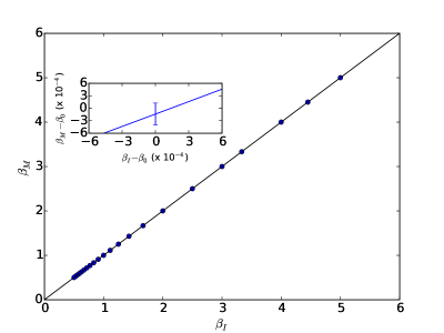
Figure 1: Measured value $\beta_{M}$ as a function of $\beta_{I}$. The inset shows a typical error bar, of order $10^{-4}$, which is not observable in the main plot.

The remarkable agreement between $\beta_{I}$ and the average of its microscopic estimator lets us conclude that the microscopic estimator $\hat{\beta}$ is indeed a trustable and robust quantity to check whether the thermal averages indeed correspond to the equilibrium values of the corresponding observables.

IV.2 Evolution towards thermal equilibrium

An advantage of our approach is that the estimator for $\beta$, given by Eq. 20, can be used to monitor the stochastic evolution towards equilibrium of the system. In Fig. 2 we show a typical thermalization process for systems of size $L$=16, $L$=32 and $L$=64 at a temperature $T$=0.4.

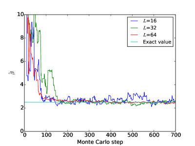
Figure 2: (Color online) Thermalization path of the dynamical temperature estimator $\hat{\beta}$ for system sizes of $L$=16, $L$=32 and $L$=64 at $T$=0.4.

We can see that the average of our estimator yields the correct inverse temperature associated to the equilibrium system, which corresponds to the input value $\beta_{I}$. In all cases equilibration occurs quickly, well within 500 Monte Carlo steps. It also holds that the larger the system, the smaller the fluctuation, as one would expect from finite-size scaling arguments. As Fig. 2 shows, the thermalization process turned out to be faster for larger systems at $T=0.4$, in spite of the general statement that larger systems require a larger number of thermalization sweeps LeBellac2004 ; Janke2008 .

The instantaneous value at every Monte Carlo step could be interpreted as the evolution of the system towards equilibrium. This is an interesting feature because, in a standard simulation, even if the average of some observable reaches a stationary regime, it does not necessarily correspond to the true equilibrium average. This may occur, for instance, in metastable systems, such as non-extensive systems Pluchino2004 . Our estimator provides an astringent test that the simulated system has thermalized, in the sense that the averages are compatible with the ones computed using the Gibbs distribution.

IV.3 Statistical independence and consistency checks

Due to the fact that the 2$d$ XY-model is critical in the whole region below $T_{BKT}$, i.e. it has infinite correlation length in the thermodynamic limit, we have used a Wolff uni-cluster algorithm aiming to reduce critical slowing down. In order to ensure the statistical independence of the generated configurations, we have implemented different tests of consistency.

IV.3.1 Autocorrelation

Firstly, the autocorrelation function of the magnetization, energy and inverse temperature were measured, from which we have obtained an estimation for the decorrelation time. For two values of temperature, namely $T$=0.2 and $T$=0.7, we performed longer simulations, with $n$=8$\times$10⁷ Monte Carlo sweeps. We have, for these temperatures, samples of energy, magnetization and $\beta$ which are known to be correlated because of the intrinsic Markov dynamics implemented in the Monte Carlo simulation. For every observable $O$, in our case the energy $E$, the magnetization $M$, and the inverse temperature $\beta$, we first computed the autocorrelation function

$$C_{O}(t)=\frac{\Big{<}O_{i}O_{i+t}\Big{>}-\Big{<}O\Big{>}^{2}}{\Big{<}O^{2}\Big{>}-\Big{<}O\Big{>}^{2}},$$ (22)

which is plotted as a function of $t$ in Fig. 3. We note that, in all cases, the correlation becomes negligible for $t\geq 2^{10}$. Also, the estimator of $\beta$ takes slightly more time to lose correlation than the other observables. In this sense, it is a more astringent estimator for statistically independence of the data.

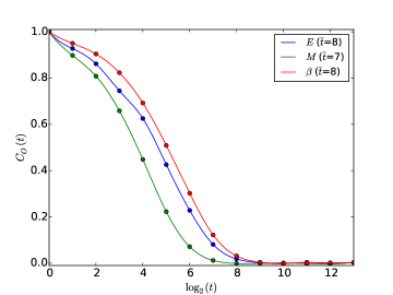
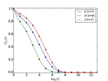
Figure 3: (Color online) Autocorrelation function $C_{O}(t)$ for energy $E$, magnetization $M$ and inverse temperature $\beta$ as a function of $\log_{2}(t)$ for temperature $T$=0.2 (upper panel) and $T$=0.7 (lower panel).

IV.3.2 Binning analysis and central limit theorem

In order to study the statistical properties of the estimator $\hat{\beta}$, we have performed, as a second independent test, a binning analysis according to the method outlined for instance, in Refs. Kawashima1994 ; Palma2015 , for temperatures $T$=0.2 and $T$=0.7.

In this method, we divide the sequence of values of an observable $O$ into blocks of size $k$, so that the total number of blocks is $N_{B}=\text{int}(n/k)$, where the int function returns the integer part of its argument. If we denote the average of the values in the $i$-th block by $\bar{O}_{i}$, the variance of these block averages is

$${\sigma_{B}}^{2}(k)=\frac{1}{N_{B}-1}\sum_{i=1}^{N_{B}}(\bar{O}_{i}-\bar{\bar{O}})^{2}.$$ (23)

where $\bar{\bar{O}}$ is the average of all block averages,

$$\bar{\bar{O}}=\frac{1}{N_{B}}\sum_{i=1}^{N_{B}}\bar{O}_{i}.$$ (24)

Under the assumption of statistical independence between the different blocks, the variance ${\sigma_{B}}^{2}(k)$ should be inversely proportional to $k$, and therefore ${\sigma_{B}}^{2}(k)/N_{B}$ should reach a constant value. As we increase $k$, we expect that we approach the regime where the block averages are really independent from each other. This gives a practical test for the minimal block size $k$ that achieves statistical independence. Fig. 4 shows this analysis for the observables $E$, $M$, and $\beta$. We see that, as we increase $k$, around $k$=2¹³=8192 the quantity ${\sigma_{B}}^{2}(k)/N_{B}$ normalized by ${\sigma_{B}}^{2}(1)$ reaches a plateau, which is consistent with a decorrelation time $t\approx$ 2¹⁰=1024.

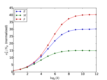
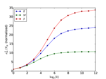
Figure 4: (Color online) Binning analysis for energy $E$, magnetization $M$ and inverse temperature $\beta$, for $T$=0.4 (upper panel) and $T$=0.7 (lower panel).

Finally, to test that the sizes of the thermal averages were large enough to produce independent statistics, we have computed the probability density function of the set of values obtained for the average of the magnetization. We checked the distribution of block averages by constructing histograms of those averages with block size $k$=2¹³, which are shown in Fig. 5. It can be observed that the histograms approach a Gaussian distribution as predicted by the central limit theorem. This criterion gives an estimation for the decorrelation time $\tau$, which is consistent with the one obtained by the binning analysis.

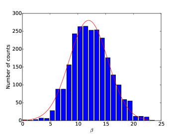
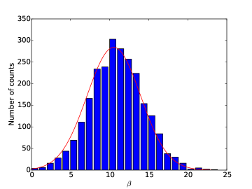
Figure 5: (Color online) Histograms of block averages of $\hat{\beta}$ for $T$=0.4 (upper panel) and $T$=0.7 (lower panel) compared to the corresponding Gaussian distribution represented by the full, red line.

V Conclusions

In this article we have shown how to construct ensemble-free microscopic estimators for the inverse temperature. We have demonstrated the practical usefulness of this estimator by simulating the two dimensional XY-model in the canonical ensemble. Among other advantages, measuring this estimator directly as a thermal average over configurations allows to monitor the transit to equilibrium of the underlying Markov process used in the Monte Carlo simulation.

The robustness of the microscopic estimator can be assessed by comparing the inverse temperature $\beta_{I}$ and $\beta_{M}$, resulting in a remarkable agreement in the whole region of relevant temperatures. The error bars turned out to be very small, and they represent absolute errors, which give valuable information about the efficiency of the algorithm utilized and about the stochastic dynamics.

The idea of constructing ensemble-free microscopic estimators could be extended to other intensive properties such as pressure, chemical potential and magnetic field, which may be useful to monitor equilibrium properties of metastable systems.

References

- (1) H. H. Rugh. Dynamical approach to temperature. Phys. Rev. Lett., 78:772, 1997.
- (2) H. H. Rugh. A geometric, dynamical approach to thermodynamics. J. Phys. A: Math. Gen., 31:7761–7770, 1998.
- (3) O. G. Jepps, G. Ayton, and D. J. Evans. Microscopic expressions for the thermodynamic temperature. Phys. Rev. E, 62:4757–4763, 2000.
- (4) G. Rickayzen and J. G. Powles. Temperature in the classical microcanonical ensemble. J. Chem. Phys., 114:4333, 2001.
- (5) B. D. Butler, G. Ayton, O. G. Jepps, and D. J. Evans. Configurational temperature: Verification of Monte Carlo simulations. J. Chem. Phys., 109:6519, 1998.
- (6) A. Baranyai. On the configurational temperature of simple fluids. J. Chem. Phys, 112:3964–3966, 2000.
- (7) W. B. Nurdin and K. D. Schotte. Dynamical temperature for spin systems. Phys. Rev. E, 61:3579, 2000.
- (8) Y. Nambu. Generalized hamiltonian dynamics. Phys. Rev. D, 7, 1973.
- (9) W. B. Nurdin and K.-D. Schotte. Dynamical temperature study for classical planar spin systems. Physica A, 308:209–226, 2002.
- (10) E. T. Jaynes. Information theory and statistical mechanics. Phys. Rev., 106:620–630, 1957.
- (11) S. Davis and G. Gutiérrez. Conjugate variables in continuous maximum-entropy inference. Phys. Rev. E, 86:051136, 2012.
- (12) S. Davis and G. Gutiérrez. Applications of the divergence theorem in Bayesian inference and MaxEnt. arXiv:1602.02544 [cond-mat.stat-mech], 2016.
- (13) C. Itzykson and J. M. Drouffe. Statistical Field Theory. Cambridge University Press, 1989. Cambridge Monographs on Mathematical Physics.
- (14) M. Le Bellac. Quantum and Statistical Field Theory. Oxford University Press, New York, 1991.
- (15) J. J. Binney, N. J. Dowrick, A. J. Fisher, and M. E. J. Newman. The theory of Critical Phenomena and Introduction to the Renormalization Group. Oxford University Press, 1992.
- (16) G. Palma, F. Niedermayer, Z. Rácz, A. Riveros, and D. Zambrano. Finite-size corrections to scaling of the magnetization distribution in the 2d xy-model at zero temperature. arXiv:1604.00948 [cond-mat.stat-mech], 2016.
- (17) U. Wolff. Collective Monte Carlo updating for spin systems. Phys. Rev. Lett., 62:361–364, 1989.
- (18) M. Le Bellac, F. Mortessagne, and G. G. Batrouni. Equilibrium and Non-Equilibrium Statistical Mechanics. Cambridge University Press, UK, 2004.
- (19) W. Janke. Monte Carlo methods in classical statistical physics. In Lecture Notes in Physics, volume 739, pages 79–140. Springer, 2008.
- (20) A. Pluchino, V. Latora, and A. Rapisarda. Metastable states, anomalous distributions and correlations in the HMF model. Physica D, 193:315–328, 2004.
- (21) N. Kawashima, J. E. Gubernatis, and H. G. Evertz. Loop algorithms for quantum simulations of fermion models on lattices. Phys. Rev. B, 50:136, 1994.
- (22) G. Palma and A. Riveros. Meron-cluster simulation of the quantum antiferromagnetic Heisenberg model in a magnetic field in one- and two-dimensions. Condensed Matter Physics, 18:23002, 2015.