Relativistic quasi-solitons and embedded solitons with circular polarization in cold plasmas
Abstract
The existence of localized electromagnetic structures is discussed in the framework of the 1-dimensional relativistic Maxwell-fluid model for a cold plasma with immobile ions. New partially localized solutions are found with a finite-difference algorithm designed to locate numerically exact solutions of the Maxwell-fluid system. These solutions are called quasi-solitons and consist of a localized electromagnetic wave trapped in a spatially extended electron plasma wave. They are organized in families characterized by the number of nodes of the vector potential and exist in a continuous range of parameters in the plane, where is the velocity of propagation and is the vector potential angular frequency. A parametric study shows that the familiar fully localized relativistic solitons are special members of the families of partially localized quasi-solitons. Soliton solution branches with are therefore parametrically embedded in the continuum of quasi-solitons. On the other hand, geometric arguments and numerical simulations indicate that solitons exist only in the limit of either small amplitude or vanishing velocity. Direct numerical simulations of the Maxwell-fluid model indicate that the quasi-solitons (and embedded solitons) are unstable and lead to wake excitation, while quasi-solitons appear stable. This helps explain the ubiquitous observation of structures that resemble solitons in numerical simulations of laser-plasma interaction.
pacs:
52.27.Ny, 52.35.Sb, 52.38.-r, 52.65.-yI Introduction
Relativistic solitary waves are localized structures consisting of a light wave trapped in a self-generated plasma cavity. They have received considerable attention over the past decade both due to their theoretical interest and their experimental relevance. Relativistic solitary waves have been found as exact solutions of the Maxwell-fluid model both in 1-dimension, with circular Kozlov et al. (1979); Kaw et al. (1992); Esirkepov et al. (1998); Farina and Bulanov (2001); Sánchez-Arriaga et al. (2011, 2011), and linear Sánchez-Arriaga et al. (2015) polarization as well as in 2-dimensions Sánchez-Arriaga and Lefebvre (2011). As observed in numerical simulations Bulanov et al. (1992, 1999); Esirkepov et al. (2002); Wu et al. (2013) and experiments Borghesi et al. (2002); Chen et al. (2007); Pirozhkov et al. (2007); Sarri et al. (2010); Sylla et al. (2012), these structures are easily excited during the interaction of high-intensity lasers with plasmas. Although the underlying mathematical model is non-integrable, they are normally referred as solitons instead of solitary waves, a term that will be used in this work.
This work studies 1-dimensional circularly polarized solitons, which are probably the solutions that received the greatest attention in the past. In Ref. Esirkepov et al. (2002) an analytical solution for standing solitons was found in the case of immobile ions. It was shown that this solution exists within the continuous range , where is the normalized frequency of the vector potential (Sect. II discusses our normalizations). Ref. Farina and Bulanov (2001) showed that solitary waves with velocity are organized in branches in the plane for both mobile and immobile ions. Each branch corresponds to a solution with a different number of zeros or nodes of the vector potential. A large number of branches were computed in Refs . Poornakala et al. (2002); Xie and Du (2006). The maximum amplitude of the waves, where the branches end, correspond to nonlinear wave breaking. This mechanism has been proposed to generate fast ions Farina and Bulanov (2001). Ion (electron) dynamics is behind the wave breaking of the low-node-number (high-node-number) waves.
The continuous spectrum of single-humped () standing waves () Esirkepov et al. (2002) and the discrete spectrum of moving () waves Farina and Bulanov (2001) led to a natural question: does a smooth transition exist between both cases? The results of Ref. Farina and Bulanov (2001) indicated a negative answer, since no moving solitons with were identified. On the other hand, in Ref. Poornakala et al. (2002), the authors gave a positive answer on the basis of numerical studies and concluded that a continuous spectrum exists for moving solitary waves with . In other words, it was claimed that, for a given value of the velocity, finite amplitude solitons moving with finite velocity exist within a certain frequency range. In the limit this family would be a continuation of the solitons (which exist for ), while in the small amplitude limit it would be a continuation of nonlinear Schrödinger equation (NLS) solitons. While later works Farina and Bulanov (2005); Saxena et al. (2006, 2007) accepted the existence of a continuous spectrum of solitons, we show in Sec. III that such a spectrum would contradict general geometric arguments from the theory of reversible dynamical systems Champneys (1998); Mielke et al. (1992). Through a detailed numerical study we show that a continuous spectrum of moving solitons exists only in one of the two integrable limits of the cold fluid model: (1) of small amplitude solutions, (2) of vanishing velocity .
A further question then arises: how are we to reconcile the ubiquitous observation of finite-amplitude structures that resemble moving solitons in numerical simulations with the fact that such solutions only exist in the small amplitude limit? As we show in Sec. IV, a more general class of partially localized solutions of the Maxwell-fluid system exists. The electromagnetic field in these solutions is localized; however, the plasma density depression exhibits non-vanishing oscillations at its tail. By analogy to similar solutions that have been observed in nonlinear optics, we refer to such solutions as quasi-solitons. The familiar soliton solution branches are parametrically embedded inside the continuous spectrum of quasi-soliton solutions. Moreover, our numerical simulations indicate that quasi-solitons are stable; this helps shed light to the abundance of such structures in laser-plasma interaction simulations.
This paper is organized as follows. Section II introduces the Maxwell-fluid model and the dynamical system associated with solitons with fixed ions. The properties of this dynamical system are summarized with emphasis at its conservative and reversible character. These properties are used in Sec. III.1 to justify the organization of the solitons in branches. Section III.2 introduces a useful algorithm that can be used to locate all the branches of solitons and shows that solitons (and the continuous spectrum) only exist in the small amplitude limit. These results are extended to plasmas with mobile ions in the Appendix. In Sec. IV a numerical algorithm to locate exact solutions is formulated and used to locate new families of quasi-solitons. It is shown that the branches of solitons are parametrically embedded inside the continuous spectrum of quasi-solitons. The stability of these structure is explored in Sec. IV.3 and our conclusion are presented in Sec. V.
II The fluid model
We consider a plasma consisting of electrons and immobile ions. For convenience, length, time, velocity, momentum, vector and scalar potentials and density are normalized by , , , , and , respectively. Here , , and are the unperturbed plasma density, the electron plasma frequency, the electron mass and the speed of light. Maxwell (in the Coulomb gauge) and plasma equations then read in the laboratory frame
| (1a) | |||
| (1b) | |||
| (1c) | |||
| (1d) |
where and are the vector and scalar potentials, is the electron plasma density, , and and are the electron momentum and velocity, respectively.
Assuming 1-dimensional () solitons, one finds from Eq. (1d) that , and
| (2a) | |||
| (2b) | |||
| (2c) | |||
| (2d) | |||
| (2e) |
We are interested in solutions of the form
| (3) |
with
| (4) |
, , and and boundary conditions , , and as (or ). Under these assumptions Eq. (2a) and (2e) become two ordinary differential equations Kozlov et al. (1979); Kaw et al. (1992); Farina and Bulanov (2001)
| (5a) | |||
| (5b) |
where the prime denotes derivative with respect to and we introduced the auxiliary functions
| (6) |
and
| (7) |
Once and are known, the fluid variables are computed from
| (8) | ||||
| (9) | ||||
| (10) |
Equations Eqs. (5a)–(5b) have several properties that are useful when discussing the existence of solitary waves. First, they result from the Hamiltonian
| (11) |
where the momenta are and . Since does not depend on explicitly, it is a conserved quantity. For our boundary conditions we have . In addition, the system is reversible in the sense defined by Devaney Devaney (1976): there is a reversing involution (a discrete symmetry operation) which fixes half the phase variables and under which the system is invariant under -reversal (). In other words, writing Eqs. (5a)-(5b) as with , there is an involution that satisfies
| (12) |
where the subspace is called the symmetric section of reversibility. Equations 5a-5b have two involutions. The first one is
| (13) |
with symmetric section
| (14) |
and the second
| (15) |
with symmetric section
| (16) |
Note also that the subspace , corresponding to pure electrostatic excitations, is invariant.
Equations (5a)–(5b) are singular when . For such a case, one readily finds from Eq. (2b) and (2e) that and . Using these results in Eq. (2d) gives the invariant
| (17) |
that provides a relation between and . A differential equation for the latter is found by combining Eq. (2a) and (2c) to yield
| (18) |
Equation (18) has the first integral
| (19) |
and also admits the two involutions and . Equation (18) admits the solitary wave solution Esirkepov et al. (2002)
| (20) |
with maximum amplitude
| (21) |
These standing solutions exist for . The soliton with maximum amplitude, exhibiting zero electron density at its center, has .
III Organization of solitons in parameter space
III.1 Geometric Arguments
Solitons of the cold fluid model described by Sys. (2e) can be found as homoclinic orbits of Eqs. (5a)–(5b), i.e. solutions that are asymptotic to a fixed point in both . Even without computing them analytically or numerically, their organization in parameter space can be anticipated by using arguments based on the dimension of the phase space, the number of conserved quantities, reversibility properties, and the dimensions of the stable and unstable manifolds of the fixed point. We recall that the stable (unstable ) manifold of a fixed point is the set of forward (backward) in trajectories that terminate at the fixed point. Since the solitons are homoclinic orbits that connect to as , these orbits lie in the intersection of and . Moreover, the solitons studied here are invariant under the -reversion transformations or [Eqs. (13)–(15)] and this implies that and have to intersect on one of the sections or defined by Eqs. (14)–(16). In Ref. Farina and Bulanov (2001) the solitons are clasified according to the number of zeros of the vector potential (number of nodes). Solitons with an even (odd) number of nodes are invariant under () and thus intersect with (). This later result will be used hereafter to discuss the existence of solitons. Interested readers can find an excellent review of the theory in Ref. Champneys (1998).
Let us first examine the case . Linearizing Eqs. (5a)–(5b) about the fixed point gives
| (22) |
| (23) |
Looking for solutions of the form , one finds that Eqs. 22 and 23 have eigenvalues and , respectively. Hereafter we restrict the analysis to , when the fixed point is a saddle-center and solitons can exist. For such a case, the stable and unstable manifolds of the fixed point are one-dimensional. By -reversibility one can see that if the unstable manifold intersects any of the symmetric sections or , then the stable manifold has to also intersect it at the same point (in fact, this implies that since both manifolds are one-dimensional). Therefore, the condition for existence of a homoclinic orbit is that the one-dimensional (or ) intersect the two-dimensional section within the three-dimensional energy shell . In general Champneys (1998), such an intersection is expected to occur for specific parameter values that form branches in the - parameter space.
For , the dynamics is governed by Eq. (18) and the phase space is two-dimensional. One readily verifies that is a fixed point with eigenvalues . If , then is a saddle and the dimensions of and are both equal to 1. The intersection of the one-dimensional unstable manifold with the one-dimensional section within the two-dimensional phase space is robust against parameter variations. This implies that solitons exist within a continuous range of . This is in agreement with the analytical solution [Eq. (20)] that exists within the frequency domain .
The previous discussion highlights the crucial difference between standing and moving solitons: the existence of the invariant if [Eq. (17)] which restricts the dimensionality of phase-space and leads to a continuous spectrum in that case. Equations (5a)-(5b) share a set of properties that are compatible with the hypothesis assumed in Ref. Mielke et al. (1992): Hamiltonian structure, reversibility, saddle-center fixed point and the invariant subspace . In addition to the cascade of homoclinic orbits and a rigorous investigation of the structure of the set made by parameter values yielding localized structures, Ref. Mielke et al. (1992) also proved the existence of families of periodic orbits and Smale horseshoes in nearby level sets of the Hamiltonian function. The latter proves that the system is not integrable globally. For this reason a global invariant in the case that could play the role of Eq. (17) for is not possible.
III.2 Numerical method to locate solitons
This section introduces a procedure to locate solitons and explains why past works concluded that there is a region in the plane with a continuous spectrum. For any given value of the parameters and we carried out integrations of Eqs. 5a and 5b with a symplectic fourth order Runge-Kutta-Nystrom method. We took an initial condition that belongs to the linear approximation of the unstable manifold of . This approximation reads
| (24) |
with a small parameter. The integrations were stopped at , when the orbit intersects the section with a tolerance smaller than . The algorithm used a fixed -step (), except at the last point of the orbit. For the latter, the Newton-Raphson method was used to find a such that was satisfied with the prescribed tolerance. All the calculations were carried with and in order to check the convergence of the results.
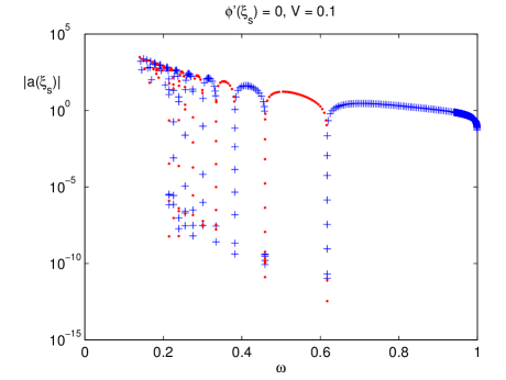
Figure 1 shows the magnitude of versus for integrations started with the initial condition Eq. (24) and parameter values ( and ) that belong to the domain where a continuous spectrum has been predicted. As shown in Fig. 1, for the distance from the symmetric section remains constant. If a soliton existed for this set of parameters, the magnitude of should vanish as . We remark that any computational method with a tolerance above would interpret this orbit, which is not homoclinic, as a soliton.
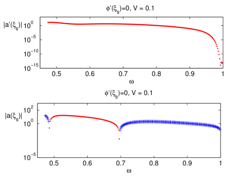
In order to investigate further the organization of the solitary waves in the plane we fixed , and carried out integrations for several values and initial conditions given by Eq. (24) with . Again we stopped the integration at , i.e. when the orbit intersected the section . At each value we recorded the value of . Figure 2 shows the absolute value of in logarithm scale versus . Crosses (dots) were used to present positive (negative) values of . The figure shows that, for , the sign of changes at several values, with the interval between two sign changes becoming smaller as decreases. Obviously, at each change of sign, there is an value, say , that makes and this designates a trajectory that intersects the section (p is even), i.e. a soliton. Since solitons occur at discrete values of for a given , the solitons are organized in branches in the plane.
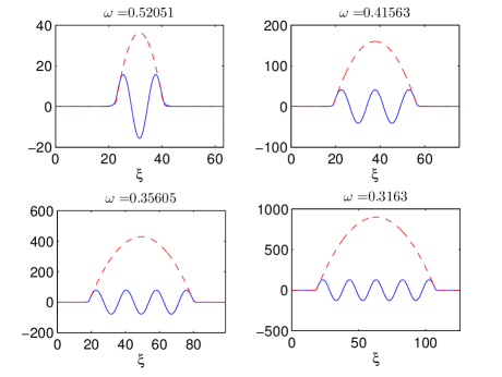
The diagram shown in Fig. 2 can be used to compute the branches with even . Once a change of sign of is detected, the value of can be computed easily with a bisection method. Figure 3 displays four examples at computed with this method. Each soliton in Fig. 3 belongs to a different branch. Branches with lower value of have a vector potential with a higher number of zeros and also much higher amplitudes.
As approaches to , decreases monotonically (see Fig. 2) but we do not observe a clear indication of an intersection with the symmetric section . Beyond a certain , say , the monotonic decrease of appears to be disrupted and we observe erratic changes in sign of . A detail of this part of the diagram is shown in Fig. 4, which contains calculations with and . We find that the onset of this effect appears at a larger for smaller and therefore is a consequence of the truncation of the infinite domain in our calculation, i.e. the finite value of in Eq. 24. The numerical integrations were started at a distance from and along a linear approximation of the unstable manifold. For this reason, we cannot expect that the behavior of versus will be smooth for . For instance, for and the erratic behavior starts when reaches about and , respectively. In order to investigate the dynamics with even closer to 1, we need to reduce more but then we are limited by the finite precision in our computations. To overcome this obstacle we use the arbitrary precision capabilities of Mathematica in order to perform computations with 30 digits of precision. We use the built-in adaptive symplectic integrator with an (absolute) error tolerance of 25 digits. This allows to verify the results obtained with with an independent code and also to perform computations with as shown in Fig. 4. We observe that the onset of erratic behavior of the sign of is now at even larger while becomes of the order of .
The trend of the curve and the geometric arguments of Sec. III.1 seem to rule out the existence of a continuous spectrum of finite amplitude solitons. In particular, there appears to be no -independent value signifying transition to such a continuous spectrum. What the behavior of as seems to indicate is that solitons exist in the small amplitude limit. Indeed, in the limit of (small solution amplitude) a nonlinear Schrödinger equation (NLS) limit of the Maxwell-fluid model exists Siminos et al. (2014) which supports soliton solutions. However, one has to note that the NLS equation is integrable, possesses infinitely many integrals of motion, thus naturally leading to the existence of solitons.
Plotting the absolute value of (instead of ) versus in logarithm scale and using crosses and dots to denote positive and negative values of reveals the organization of the solitons with odd (see Fig. 5). These are orbits that intersect the section. There are many changes of sign of and, at the particular values that make , there are branches of solitons with an odd number of nodes in the vector potential. Some of these orbits are shown in Fig. 6.
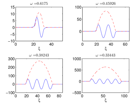
Tables 1 and 2 summarize some of the numerical results for . It contains branches of solutions with the number of zeros of the vector potential from 1 to 20 as well as the frequency values which give rise to localized solitons.
| p | ||
|---|---|---|
| 2 | 0.52050770 | |
| 4 | 0.41562715 | |
| 6 | 0.35604770 | |
| 8 | 0.31629641 | |
| 10 | 0.28736027 | |
| 12 | 0.26509070 | |
| 14 | 0.24727222 | |
| 16 | 0.23259912 | |
| 18 | 0.22024540 | |
| 20 | 0.20965960 |
| p | ||
|---|---|---|
| 1 | 0.61749714 | |
| 3 | 0.45926068 | |
| 5 | 0.38242601 | |
| 7 | 0.33443103 | |
| 9 | 0.30080027 | |
| 11 | 0.27555955 | |
| 13 | 0.25572137 | |
| 15 | 0.23960230 | |
| 17 | 0.22617167 | |
| 29 | 0.21475857 |
IV Quasi-solitons and embedded solitons
As we now show, the solitons computed in Sec. III are special members of a new family of delocalized solutions named quasi-solitons. The latter do not only provide a broader understanding of the former but also have an interesting physical meaning. In general, quasi-soliton are weakly non-localized solutions with a soliton-like core and non-vanishing oscillatory tails Boyd (1998). In the present case, the quasi-solitons that we will find are partially localized: the electromagnetic field is localized but the longitudinal quantities, e.g. and exhibit oscillatory tails.
From a dynamical system point of view, a quasi-soliton is an homoclinic orbit that connects at with a periodic orbit. In a reversible Hamiltonian system like Eq. (5a)-(5b), the existence of a quasi-soliton requires the intersection of the 2-dimensional unstable manifold of the periodic orbit with the 2-dimensional symmetric section. Hence, symmetric quasi-solitons are persistent under parameter variations and they would appear in a continuous region of the plane Champneys (1998). As shown in the context of nonlinear optics Yang et al. (1999), the amplitudes of the oscillating tails of the quasi-solitons can exactly vanish at a discrete set of parameter values. In other words, for certain relations these solutions are truly localized and correspond to branches of true solitons. For this reason, such solitons are said to be parametrically embedded in the family of delocalized quasi-soliton.
Before we explore if this mechanism also applies in our problem we note that since we found Eqs. (5a)-(5b) from Eqs. (2a)-(2e) by imposing the boundary conditions , , and as , only solutions of Eqs. (5a)-(5b) connecting with the equilibrium point correspond to solutions of the fluid system given by Eqs. (2a)-(2e). However, quasi-solitons connect with a periodic orbit and not with . For this reason, we will compute quasi-soliton solutions directly from Eqs. (2a)-(2e) with an extension to of the finite-difference algorithm presented in Ref. Sánchez-Arriaga et al. (2015).
IV.1 Numerical algorithm to locate quasi-solitons
Since this work deals with traveling waves, we introduce a boosted frame that moves with constant velocity along the -axis. Four-vectors , , and with the electron charge and current densities given by and transform according to Lorentz transformations. Equations Eqs. (2a)–(2e) in the boosted frame read
| (25a) | |||
| (25b) | |||
| (25c) | |||
| (25d) | |||
| (25e) |
where we used a prime to denote the variables in the boosted frame and introduced the normalized distance and time
| (26) |
For numerical convenience we also introduced the parameters and , which allow to work in a computational box and .
Quasi-solitons are spatially- and temporally-periodic solutions of Eq. (25e) with unknown spatial period and angular frequency . We note that we do not impose a restriction on the functional form of these solutions as we did in writing Eq. (3). In our algorithm the computational box is discretized with and regularly spaced points. A vector of unknowns with and with the values of the variables at the grid points is constructed. After using second order finite-difference formulae to approximate the spatial and temporal derivatives and imposing periodic boundary conditions in space and time, one finds from Eq. (25e) a large set of nonlinear algebraic equations of the form
| (27) |
for the unknowns ( and are treated as fixed parameters). This is solved iteratively with a Newton-Raphson method, using as initial guesses the soliton solutions computed in Sec. III or the analytical solution given in Eq. (20). Our algorithm takes advantage of the sparsity of the Jacobian of , which was computed analytically, and it carries out its LU factorization using parallel computation. In our calculations we used , and a solution was accepted as valid if the tolerance of the Newton method, i.e. the residual of Eq. (27), was smaller than .
IV.2 Quasi-soliton solutions
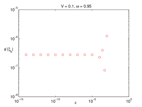
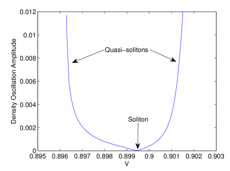
We now provide examples of the use of the numerical algorithm of Sec. IV.1 in order to locate quasi-solitons. Using the method introduced in Sec. III we find that, for , there is a soliton solution with at . We then use these parameter values and , with the code described in Sec. IV.1 and compute a solution using as initial guess the spatiotemporal profile found through the integration of Eqs. (5a)–(5b) and the use of Eq. (3) and (8)-(10). We then use the velocity as continuation parameter to compute quasi-solitons with . At each value of , the code used as initial guess the quasi-soliton solution found at the previous velocity value.
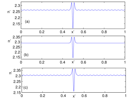
Figure 7 shows the relative (mean value was subtracted) amplitude of the density oscillations at the quasi-soliton tail versus the velocity at . The amplitude of the density oscillations at the tail is equal to at . The limiting factor in our computations is the discretization error in space which is . Therefore, this result is in agreement with the solution of Eqs. (5a)–(5b), i.e. a fully localized solution at . Panels (a)-(c) in Fig. 8 display the electron density profile of quasi-solitons with and velocity and , respectively. The oscillations at the tail except at a particular value of [panel (b)] are evident. The wavelengths of the oscillations at the tail are in agreement with the linear analysis of Sec. III.1. They are about , i.e. they correspond to the eigenvalues that are associated with small amplitude oscillations of according to Eq. (23). These numerical calculations demonstrate that the branches of solitons are parametrically embedded at the continuous spectrum of the quasi-soliton.
.
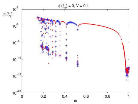
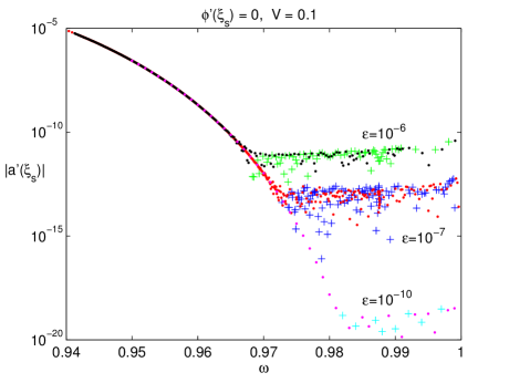
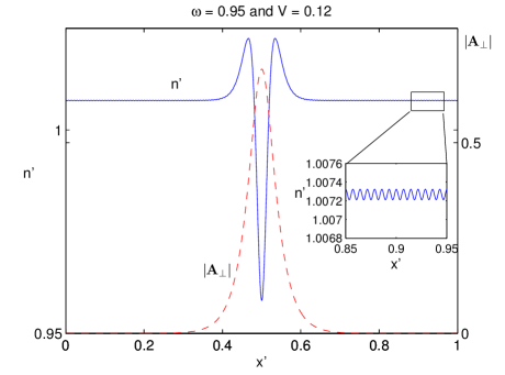
The existence of quasi-solitons with finite velocity was also investigated with the finite-difference code. For these calculations we set , and used as a continuation parameter. The analytical solution given by Eq. (20) was used as initial guess. Solutions where found in a continuous range of ; as an example, we show in Fig. 9 a quasi-soliton with , thus giving numerical evidence of the existence of this special type of quasi-soliton. The inset shows that small amplitude oscillations with a high-wavevector exist at the tail. This result is again in agreement with the linear analysis of Sec. III.1. As the wavelength of the tail oscillation () vanishes. As a consequence, numerical difficulties arise at this particular limit, which requires a high resolution to capture the structure of the solution appropriately.
IV.3 Stability of the quasisoliton solutions
In this section we study numerically the stability of the quasi-soliton solutions. Since these solutions are calculated with finite precision, the residual in Eq. (27) acts as a perturbation of the exact solution. Thus, integrating the Maxwell-fluid model Eq. (1d) with quasi-soliton solutions determined using the algorithm of Sec. IV.1 as initial condition provides information on their stability.
The numerical integration is performed in the lab-frame with the pseudo-spectral code described in Ref. Siminos et al. (2014). For the spatial dependence of the field and plasma quantities, Fourier space discretization is used, while time stepping is handled by an adaptive fourth order Runge-Kutta scheme. In order to ensure numerical stability a filter in Fourier space of the form is used. This prevents the growth of aliased high- modes, while the dynamics of the physically relevant modes are not affected. The solutions found in the boosted frame with the algorithm of Sec. IV.1 are transformed to the lab frame using Lorentz transformations in order to obtain the initial conditions required for the direct numerical integration.
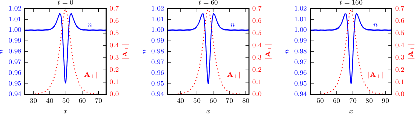
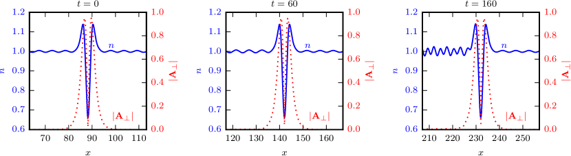
In Fig. 10 we show snapshots from the evolution of a quasi-soliton with and . We observe that the quasi-soliton remains essentially unchanged up to , indicating stability. In Fig. 11 we show the evolution of a quasi-soliton with and . An instability develops in the trailing edge of the density profile. This instability is similar to the one observed in fluid simulations of solitons Saxena et al. (2006) and connected to the forward stimulated Raman scattering instability Saxena et al. (2007). The disturbance of the wake leads to radiation of part of the electromagnetic field of the soliton. We note that ion motion, not included here, is expected to also play a role in quasi-soliton evolution, in particular for small , as already seen in studies of soliton stability at the ion time scale Lehmann et al. (2006). A more comprehensive study of the stability of quasi-solitons is beyond the scope of this work and will be presented in a future publication.
V Conclusions
We have shown that quasi-soliton solutions of the Maxwell-fluid model exist in continuous domains of the plane. These solutions consist of a localized electromagnetic pulse with number of nodes of the vector potential trapped in a plasma density cavity with oscillations at its tails. Our study also sheds light to the organization in parameter space of the circularly polarized relativistic solitons identified in previous studies. The solitons with turn out to be special members of the corresponding quasi-soliton family for which the density tail-oscillations vanish. Therefore, such solitons exist for specific values , i.e. they form branches in the plane. This is consistent with the geometric arguments of the theory of dynamical systems which were used in Sec. III.1 to formulate a method to locate these branches. Although the values of which give rise to localized solitons are found numerically and with a finite accuracy, the bisection method developed proves rigorously their existence because it is based on zero-crossings of (even ) or (odd ). This allows to rule out the existence of a continuous spectrum for finite amplitude and finite velocity, solitons. Such a continuous spectrum only exists in either of the integrable limits of the Maxwell-fluid model, i.e. for or . However, the only proper finite amplitude and velocity solitary waves with are the quasi-solitons presented here.
Our stability study suggests that quasi-solitons are stable while ones with are unstable. This could help explain the abundance of single-humbed soliton-like structures in laser-plasma interaction. It appears rather natural that during the process of excitation of such structures, non-vanishing tail oscillations (’wakes’) are also excited by the driving laser pulse. We therefore expect that our study will prompt the identification of quasi-solitons structures in laser-plasma simulations and experiments.
Acknowledgements.
This work was supported by the Ministerio de Economía y Competitividad of Spain (Grant No RYC-2014-15357) and by the Knut and Alice Wallenberg Foundation (pliona project).Appendix A Solitons with mobile ions
For mobile ions Eqs. (5a)-(5b) read Kozlov et al. (1979)
| (28a) | |||
| (28b) |
where , and . In our calculations we will take . The system admits the Hamiltonian
| (29) | ||||
| (30) |
and the involutions Eq. (13) and Eq. (15). Since the equilibrium has eigenvalues and , solitons are expected to be organized in branches in the plane. The same numerical method used for fixed ions was used to investigate the spectrum of the solitons with mobile ions. The main difference is the initial condition that now reads
| (31) |
Figure 12 shows the Poincare maps () of (top panel) and (bottom panel ) versus for . Since the variable does not vanish, we conclude that solitons do not exist. The two zeros of correspond to the branch of solutions that has a turning point in the plane (see Ref. Farina and Bulanov (2001)).
References
- Kozlov et al. (1979) V. A. Kozlov, A. G. Litvak, and E. V. Suvorov, Soviet Journal of Experimental and Theoretical Physics 49, 75 (1979).
- Kaw et al. (1992) P. K. Kaw, A. Sen, and T. Katsouleas, Phys. Rev. Lett. 68, 3172 (1992).
- Esirkepov et al. (1998) T. Z. Esirkepov, F. F. Kamenets, S. V. Bulanov, and N. M. Naumova, Soviet Journal of Experimental and Theoretical Physics Letters 68, 36 (1998).
- Farina and Bulanov (2001) D. Farina and S. V. Bulanov, Phys. Rev. Lett. 86, 5289 (2001).
- Sánchez-Arriaga et al. (2011) G. Sánchez-Arriaga, E. Siminos, and E. Lefebvre, Phys. Plasmas 18, 082304 (2011).
- Sánchez-Arriaga et al. (2011) G. Sánchez-Arriaga, E. Siminos, and E. Lefebvre, Plasma Phys. Control. Fusion 53, 045011 (2011).
- Sánchez-Arriaga et al. (2015) G. Sánchez-Arriaga, E. Siminos, V. Saxena, and I. Kourakis, Phys. Rev. E 91, 033102 (2015).
- Sánchez-Arriaga and Lefebvre (2011) G. Sánchez-Arriaga and E. Lefebvre, Phys. Rev. E 84, 036403 (2011).
- Bulanov et al. (1992) S. V. Bulanov, I. N. Inovenkov, V. I. Kirsanov, N. M. Naumova, and A. S. Sakharov, Phys. Fluids B 4, 1935 (1992).
- Bulanov et al. (1999) S. V. Bulanov, T. Z. Esirkepov, N. M. Naumova, F. Pegoraro, and V. A. Vshivkov, Phys. Rev. Lett. 82, 3440 (1999).
- Esirkepov et al. (2002) T. Esirkepov, K. Nishihara, S. V. Bulanov, and F. Pegoraro, Phys. Rev. Lett. 89, 275002 (2002).
- Wu et al. (2013) D. Wu, C. Y. Zheng, X. Q. Yan, M. Y. Yu, and X. T. He, Phys. Plasmas 20, 033101 (2013).
- Borghesi et al. (2002) M. Borghesi, S. Bulanov, D. H. Campbell, R. J. Clarke, T. Z. Esirkepov, M. Galimberti, L. A. Gizzi, A. J. MacKinnon, N. M. Naumova, F. Pegoraro, H. Ruhl, A. Schiavi, and O. Willi, Phys. Rev. Lett. 88, 135002 (2002).
- Chen et al. (2007) L. M. Chen, H. Kotaki, K. Nakajima, J. Koga, S. V. Bulanov, T. Tajima, Y. Q. Gu, H. S. Peng, X. X. Wang, T. S. Wen, H. J. Liu, C. Y. Jiao, C. G. Zhang, X. J. Huang, Y. Guo, K. N. Zhou, J. F. Hua, W. M. An, C. X. Tang, and Y. Z. Lin, Phys. Plasmas 14, 040703 (2007).
- Pirozhkov et al. (2007) A. S. Pirozhkov, J. Ma, M. Kando, T. Z. Esirkepov, Y. Fukuda, L.-M. Chen, I. Daito, K. Ogura, T. Homma, Y. Hayashi, H. Kotaki, A. Sagisaka, M. Mori, J. K. Koga, T. Kawachi, H. Daido, S. V. Bulanov, T. Kimura, Y. Kato, and T. Tajima, Phys. Plasmas 14, 123106 (2007).
- Sarri et al. (2010) G. Sarri, D. K. Singh, J. R. Davies, F. Fiuza, K. L. Lancaster, E. L. Clark, S. Hassan, J. Jiang, N. Kageiwa, N. Lopes, A. Rehman, C. Russo, R. H. H. Scott, T. Tanimoto, Z. Najmudin, K. A. Tanaka, M. Tatarakis, M. Borghesi, and P. A. Norreys, Phys. Rev. Lett. 105, 175007 (2010).
- Sylla et al. (2012) F. Sylla, A. Flacco, S. Kahaly, M. Veltcheva, A. Lifschitz, G. Sánchez-Arriaga, E. Lefebvre, and V. Malka, Phys. Rev. Lett. 108, 115003 (2012).
- Poornakala et al. (2002) S. Poornakala, A. Das, A. Sen, and P. K. Kaw, Phys. Plasmas 9, 1820 (2002).
- Xie and Du (2006) B.-S. Xie and S.-C. Du, Phys. Scripta 74, 638 (2006).
- Farina and Bulanov (2005) D. Farina and S. V. Bulanov, Plasma Phys. Control. Fusion 47, A260000 (2005).
- Saxena et al. (2006) V. Saxena, A. Das, A. Sen, and P. Kaw, Phys. Plasmas 13, 032309 (2006).
- Saxena et al. (2007) V. Saxena, A. Das, S. Sengupta, P. Kaw, and A. Sen, Phys. Plasmas 14, 072307 (2007).
- Champneys (1998) A. R. Champneys, Physica D 112, 158 (1998).
- Mielke et al. (1992) A. Mielke, P. Holmes, and O. O’Reilly, J. Dyn. Differ. Equ. 4, 95 (1992).
- Devaney (1976) R. L. Devaney, T. Am. Math. Soc. 218, 89 (1976).
- Siminos et al. (2014) E. Siminos, G. Sánchez-Arriaga, V. Saxena, and I. Kourakis, Phys. Rev. E 90, 063104 (2014).
- Boyd (1998) J. Boyd, Weakly Nonlocal Solitary Waves and Beyond-All-Orders Asymptotics, Mathematics and Its Applications, Vol. 442 (Springer, 1998).
- Yang et al. (1999) J. Yang, B. A. Malomed, and D. J. Kaup, Phys. Rev. Lett. 83, 1958 (1999).
- Lehmann et al. (2006) G. Lehmann, E. W. Laedke, and K. H. Spatschek, Phys. Plasmas 13, 092302 (2006).