Ensemble Distribution for Immiscible Two-Phase Flow in Porous Media

Abstract

We construct an ensemble distribution to describe steady immiscible two-phase flow of two incompressible fluids in a porous medium. The system is found to be ergodic. The distribution is used to compute macroscopic flow parameters. In particular, we find an expression for the overall mobility of the system from the ensemble distribution. The entropy production at the scale of the porous medium is shown to give the expected product of the average flow and its driving force, obtained from a black-box description. We test numerically some of the central theoretical results.

I Introduction

Multiphase flow in porous media poses interesting problems to engineers and scientists in diverse fields b88 . Understanding the nature of multiphase flow is relevant to understand the flow of particles in bifurcating blood vessels, or to categorizing liquid transportation through cellulose. Other interesting areas concern diffusion of pollutants in soil, and the flow of hydrocarbons and water in oil reservoirs.

It is apparent from this wide range of applications of porous flow, that the length scale of relevant processes can range from few nanometers to several kilometers. In geological transport processes such as aquifers and oil reservoirs, this fact is especially important, as the processes that occur at the pore scale (micron scale) remain important in attempting to understand the processes at the reservoir scale (kilometer scale).

When two immiscible fluids flow simultaneously in a rigid porous medium, the state-of-the-art description is given by the relative permeability equations, which are considered to be the effective medium equations. The relative permeability approach views each fluid as moving in a pore space that is constrained by the other fluid. Hence, each fluid will experience a lowered effective permeability since it experiences a diminished pore space in which to move. The ratio between the effective permeabilities of each fluid and the single-fluid permeability of the porous medium are the relative permeabilities. The relative permeabilities are thought only to depend on the fluid saturations (which are the volumes of each fluid relative to the pore volume). In addition to the relative permeabilities, a capillary pressure field that models the interfacial tension between the two fluids is introduced wb36 .

The concept of relative permeability is simple. However, different laboratory methods, e.g. the Penn State or the Hassler method orkhb51 yield different results for the measurement of relative permeability. This signals that the relative permeability equations do not offer a complete description of the problem. These weaknesses have been known for a long time and it is not controversial to state that the relative permeability approach should and probably will be replaced by a better framework. Several attempts have been made to replace this framework, see e.g., lsd81 ; g89 ; hg90 ; hg93a ; hg93b ; gh98 ; h98 ; g99 ; hb00 ; h06a ; h06b ; h06c ; hr09 ; hd10 ; nbh11 ; dhh12 ; habgo15 ; h15 ; vd16 ; gsd16 ; hsbksv16 .

Techniques for recording and reconstructing the pore structure of porous media has developed tremendously over the last years bbdgimpp13 . It is now possible to render detailed maps of the structure of porous media at the sub-pore level.

Numerical techniques to calculate the flow properties have also developed and branched over the years. There are several approaches. Bryant and Blunt bb92 were the first to calculate relative permeabilities from a detailed network model. Aker et al. amhb98 ; kah02 developed a network model which was extended to include film flow by Tørå et al. toh12 . The model is today being combined with a Monte Carlo technique sshbkv16 to speed up the calculations considerably. A recent review summarizes the status of this class of models, see jh12 . A very different approach is the Lattice Boltzmann method rob10 ; rino12 , see also broglekawbw16 ; acbrsb16 . Whereas the network models are ideal for large network without detailed knowledge of the presice shape of each pore, the Lattice Boltzmann method has the opposite strength. It goes well with the detailed pore spaces that are now being reconstructed but is less useful in large networks. Other methods than the Lattice Boltzmann one which resolve the flow at the pore level are e.g. smoothed particle hydrodynamics tm05 ; op10 ; ll10 , and density functional hydrodynamics abdekks16 .

The goal of any theory of immiscible two-phase flow in porous media must be to bind together the physics at the pore level with a description at scales where the porous medium may be seen as a continuum. We illustrate this viewpoint through the relative permeability equations that attempt to do exactly this:

$$\vec{\nu}_{w}=-\frac{K}{\mu_{w}}\ k_{r,w}\ \vec{\nabla}P_{w}\;,$$ (1)

and

$$\vec{\nu}_{n}=-\frac{K}{\mu_{n}}\ k_{r,n}\ \vec{\nabla}P_{n}\;.$$ (2)

Here $\nu_{w}$ and $\nu_{n}$ are the Darcy velocities of the wetting and non-wetting fluids, $\mu_{w}$ and $\mu_{n}$ the viscosities of the wetting and non-wetting fluids, $K$ is the permeability of the porous medium. $k_{r,w}(s)$ and $k_{r,n}(s)$ are the relative permeabilities of the wetting and non-wetting fluids. $s$ is the non-wetting saturation. One distinguishes between the pressure in the wetting fluid $P_{w}$ and in the non-wetting fluid $P_{n}$. They are related through the capillary pressure $P_{c}(s)$ by

$$P_{n}-P_{w}=P_{c}\;.$$ (3)

The relative permeabilities and the capillary pressure are assumed to be functions of the non-wetting fluid saturation $s$ alone. These equations treat the porous medium as a continuum. There are three functions entering these three equations that are determined by the physics at the pore level: $k_{r,w}(s)$, $k_{r,n}(s)$ and $P_{c}(s)$.

An alternate recent theory hsbksv16 based on thermodynamics kb08 ; kbjg10 proposes the relations

$$\frac{d\vec{\nu}}{ds}=\vec{\nu}_{n}-\vec{\nu}_{w}\;,$$ (4)

and

$$s\ \frac{d\vec{\nu}_{n}}{ds}+(1-s)\ \frac{d\vec{\nu}_{w}}{ds}=0\;,$$ (5)

where $\vec{\nu}=s\vec{\nu}_{n}+(1-s)\vec{\nu}_{w}$ is the saturation-weighted average Darcy velocity. The pore-level physics enters the picture through the constitutive equation $\vec{\nu}=\vec{\nu}(s,\vec{\nabla}P)$, where $P$ is the pressure.

The functions $k_{r,w}(s)$, $k_{r,n}(s)$, $P_{c}(s)$, or in the last case $\vec{\nu}=\vec{\nu}(s,\vec{\nabla}P)$ are macroscopic functions; they are defined at the continuum level. Other theories will have other macroscopic functions that connect the pore level physics to the continuum level. Such functions are the results of the collective behavior of the fluids in vast numbers of pores. To be able to calculate the precise behavior of the fluids in a small number of pores as done when using Lattice Boltzmann method is not enough to determine fully the physics on large scales. This is well-known in other fields such as statistical mechanics where longe-range correlations that are generated by the short-range interactions between the microscopic components may dominate the behavior.

It is therefore tempting to develop a statistical mechanics for immiscible two-phase flow in porous media. The goal of statistical mechanics is precisely to bind the microscopic and the macroscopic worlds together, and it has been very successful doing this in the past. We will in this paper attempt to take the first steps in this direction.

In the 1950s through 60s, work was done on a statistical description of flow in porous media cc50 ; s54 ; s65 ; a66 . Since the late 80s, a theory of two-phase flow using a thermodynamic approach has been developed and employed by Hassanizadeh and Gray hg90 ; gh98 ; g99 ; g89 . More recently, Valavanides and Daras vd16 employ tools from statistical mechanics to describe flow. Hansen and Ramstad hr09 proposed to develop a thermodynamical description of immiscible two-phase flow in porous media based on the configurations of the fluid interfaces, an approach that is related to that of Valavanides and Daras.

In the spirit of Hansen and Ramstad hr09 , we aim to develop a statistical description of the flow of two immiscible fluids through a two-dimensional network by constructing a macroscopic description that applies to the ensemble-averaged behavior of all connected links. Sinha et al. shbk13 derived a statistical description of steady state two-phase flow in a single capillary tube. They showed that the well-known Washburn equation could be derived from the entropy production in the tube. They verified that the system was ergodic and derived an analytical expression for the ensemble distribution. The ensemble distribution is the probability distribution of finding the center of mass of a bubble of the non-wetting liquid at a particular position in the tube. The ensemble distribution in the one-dimensional case was found to be inversely proportional to the velocity of the non-wetting bubble. Given that a slow bubble stays proportionally longer in a link, this velocity dependence is self-evident. This idea was developed further, by demonstating in sshbkv16 that the probability for a given configuration of interfaces in a network, not just a one-dimensional one, is proportional to the inverse of the total flow through the network. This probability distribution was then used to form the basis for a Markov chain Monte Carlo method for sampling configurations in a network model.

Whereas the configurational probability distribution that was derived in Savani et al. sshbkv16 , gave the probability density for the interfaces between the fluids forming a given configuration in the entire network, we will here construct an ensemble distribution for the individual links. That is, we will derive the joint probability density for any link in the network to have a given saturation, that the non-wetting fluid it contains will have its center of mass at a given position and that its radius will have a given value.

We consider here for concreteness a network of pores each characterized by a length and a radius. We define flow velocity and saturations for each link and set up the joint statistical distribution between these and the radius distribution. We will assume that the porous medium — the network of pores — is homogeneous. This implies that if there are two statistically similar networks, the combined system will have the same properties as the separate systems.

The paper is organized as follows. In section II we describe the porous medium model we will use for the theoretical derivations. We use a biperiodic square lattice where the links model the pores. This simplifies the theoretical discussion while retaining the complexity of the flow. Section III introduces the ensemble distribution that provides the joint probability distribution for pore radius, pore saturation, and the position of bubbles in the pores. The first of these variables characterizes the porous medium whereas the other two characterize the flow. We go on to demonstrate that the ensemble distribution is inversely proportional to the volume flow through the links. We also demonstrate that the system is ergodic. The next section IV connects the ensemble distribution with dfferent macroscopic quantities, namely the fractional volume flow, the saturation, the pressure difference and the entropy production. In section V we test numerically some of the central results of the previous sections. Our conclusions are given in section VI.

II Defining the Variables Characterizing the Flow and the Porous Medium

In the same way as Bakke and Øren bo97 ; s11 extracted a network from the pore space of a porous medium, we replace the original porous medium by a network representing its pore space. All our variables will be defined with reference to the links in this network.

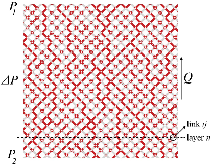
In this paper, however, we go one step further and consider a lattice in the form of a square grid. This is of course a considerable and unrealistic simplification compared to the topology of a real pore network. However, as the goal of this work is not to consider a given structure but to develop a general theory, it is convenient to use the square network. It simplifies the discussion while retaining the important subtleties. The square lattice is periodic in both directions. We orient it so that the main axes form $45^{\circ}$ with the average flow direction, see Fig. 1. There are $L\times L$ distinct links in the lattice. This means that there are $L$ distinct layers of links, see Fig. 1. For a square lattice, the total number of nodes is then $L^{2}/2$ and a link between two neigboring nodes $i$ and $j$ is denoted by $ij$ where $i,j\in[0,L^{2}/2]$.

We assume that all links in the network have the same length $l$. The radius $r_{0,ij}$ varies from link to link and is drawn from a spatially uncorrelated distribution $f_{r}(r_{0,ij})$.

A volume flow $Q$ across the network in the vertical direction generates a pressure difference across one layer $\Delta P/L$ depending on $s$ in the opposite direction, see Fig. 1.

We define the non-wetting saturation $s_{ij}$ in link $ij$ as

$$s_{ij}\equiv\frac{v_{n,{ij}}}{v_{ij}}\;,$$ (6)

where $v_{n,ij}$ refers to the volume of non-wetting fluid in the link and $v_{ij}$ is the total volume of the link.

Figure 1: The square network with a typical steady-state configuration of wetting (white) and non-wetting (red) fluids. We control the volume flow $Q$ through the network. This generates a pressure difference $\Delta P=P_{1}-P_{2}$ which depends on the saturation $s$, between the top and bottom of the network. Note that the network is biperiodic: fluid which escapes at the top enters the corresponding node at the bottom and fluid which leaves to the right enters at the left.

We assume that the wetting fluid does not wet the pores completely so that it does not form films. The non-wetting fluid will form bubbles that fill the cross-sectional area of the links. The position of the bubbles may be characterized by one number since they cannot pass or change their distance from each other. We characterize their motion through the time derivative of one position variable $x_{b,ij}$ which signifies e.g. the position of their center of mass measured along the link of length $l$. Hence $0\leq x_{b,ij}\leq l$.

We will consider steady-state flow esthfm13 . Experimentally, this is attained when the two immiscible fluids are injected simultaneously into the porous medium with all control parameters kept constant and all measured macroscopic quantities fluctuate around well-defined and constant averages. In our square lattice, the steady state is attained when the fluids are allowed to circulate long enough in the biperiodic network. The steady state does not imply that the interfaces at the pore level are static. Rather, $\Delta P$ may be so high that all interfaces move and the system would still be in the steady state.

III Ensemble Distribution

At a given moment in time, there is a certain configuration of the two fluids in the network. The ensemble distribution is derived from this snapshot and is considered to be a time-independent probability distribution of the two fluids over the ensemble of links since the flow appears under steady-state conditions. The exact nature of the ensemble distribution is still unknown, however, the aim of this work is to derive some of its properties. Such knowledge will enable the integration across the network for determining various properties of interest. For instance, we are interested in the average pressure difference and the fractional volume flow of the wetting and the non-wetting fluids when the total volume flow $Q$ and $s$ are imposed. In particular we are interested in the total volume flows of each of the single fluids. Thermodynamics on the macroscopic level has recently been used to relate these quantities hsbksv16 . However, this approach is entirely macroscopic. Using an ensemble distribution, we can build a bridge between the properties of a single link and the overall performance of the network. We aim to develop a new method that can solve the up-scaling problem in the context of immiscible multi-phase flow in porous media.

The ensemble distribution we develop in the following is at the indivual link level. That is, pick a link in the network at random. What is the joint probability density that this link has a given radius, saturation and the center-of-mass position of the non-wetting bubbles it contains is at a certain position.

As was stated in the introduction, this is different from the configurational probability distribution, that is the probability density for the interfaces between the two fluids takes on a given configuration in the network, that was derived in Savani et al. sshbkv16 and used to construct a Markov chain Monte Carlo algorithm for sampling configurations in network models.

III.1 The One-Dimensional Distribution

Working towards the goal to determine the ensemble distribution beyond one dimension, we start with conclusions from a one-dimensional sequence of links shbk13 . We have reported earlier that the probability that a bubble has a certain position $x_{b,ij}$ in the link, is inversely proportional to the velocity $dx_{b}/dt$ of the fluid in that link

$$\Pi(x_{b})=\frac{1}{\tau}\frac{1}{dx_{b}/dt}=\frac{1}{l}\frac{\langle q\rangle}{q(x_{b})}\;,\text{ \ \ \ for \ \ }0<x_{b}<l\;,$$ (7)

where $\tau=\pi{r_{0}}^{2}l/\langle q\rangle$ is the average time the bubble takes to move from one end of the link to the other end, and $\langle q\rangle$ is the average volume flow. This ensemble distribution expresses the sensible fact that the time a bubble spends in a link, is inversely proportional to its velocity.

The system characterized by ensemble distribution in equation (7) is by construction ergodic shbk13 . The time average of a function $g=g(x_{b})$ is $\overline{g}$, and we have

$$\overline{g}=\frac{1}{\tau}\ \int_{0}^{\tau}dt\ g\left(x_{b}(t)\right)=\int_{0}^{l}\ dx_{b}\ \frac{g(x_{b})}{\tau dx_{b}/dt}=\int_{0}^{l}dx_{b}\ \Pi(x_{b})\ g(x_{b})=\langle g\rangle\;.$$ (8)

Hence, the time average of any function equals its ensemble average — which is the definition of ergodicity.

III.2 Ensemble distribution in higher dimesions

In higher dimensions, at any instance, the state of a link can be characterized by the center-of-mass position of the bubbles in it, $x_{b,ij}$, the saturation $s_{ij}$, and the radius $r_{0,ij}$ of the link. In the course of time, a single link will see the passage of many bubbles with different sizes. One may calculate the time average of $q_{ij}$ for each individual link.

A subsequent average over the radii of the links returns the average volume flow $\langle q\rangle$ in the links. A fast bubble will spend proportionally less time in a given link than a slow bubble. This is true whether the link is part of a one-dimensional or a multi-dimensional network. This suggests that also in the multi-dimensional case, the ensemble distribution, $\Pi(x_{b,ij},s_{ij},r_{0,ij})$, will be inversely proportional to the volume flow $\left|{q_{ij}(x_{b,ij},s_{ij},r_{0,ij})}\right|$. By the same argument that led to equation (8) and hence, ergodicity, the multidimensional system must be ergodic.

A general form of the ensemble distribution is

$$\Pi(x_{b,ij},s_{ij},r_{0,ij}) =\frac{\langle\left|q\right|\rangle}{\left|q_{ij}(x_{b,ij},s_{ij},r_{0,ij})\right|}f(x_{b,ij},s_{ij},r_{0,ij})$$ (9)

$$\text{for}\ 0<x_{b,ij}<l\ \text{and}\ 0<s_{ij}<1\;,$$

where $f(x_{b,ij},s_{ij},r_{0,ij})$ is assumed to be normalized. The distribution $f(x_{b,ij},s_{ij},r_{0,ij})$ may, in principle, depend on the volume flow $q_{ij}(x_{b,ij},s_{ij},r_{0,ij})$. If $f(x_{b,ij},s_{ij},r_{0,ij})$ does not depend on $x_{b,ij}$ via its flow dependence, the implication is that $f(x_{b,ij},s_{ij},r_{0,ij})$$=f(s_{ij},r_{0,ij})/l$. It then follows that the ensemble distribution takes the form

$$\Pi(x_{b,ij},s_{ij},r_{0,ij}) =\frac{1}{l}\frac{\langle\left|q\right|\rangle}{\left|q_{ij}(x_{b,ij},s_{ij},r_{0,ij})\right|}f(s_{ij},r_{0,ij})$$

$$\text{for}\ 0<x_{b,ij}<l\ \text{and}\ 0<s_{ij}<1\;.$$ (10)

The function $f(s_{ij},r_{0,ij})$, which is also normalized, gives the joint distribution of the saturation and the link radii.

IV From ensemble distribution to macroscopic quantities

The aim of this section is to calculate the fractional volume flow of the non-wetting fluid, the saturation, the pressure drop and the entropy production, all macroscopic variables, from the ensemble distribution.

IV.1 Average Absolute Volume and Fractional Volume Flows

The average absolute volume flow is given by

$$\langle\left|q\right|\rangle\ =\int_{0}^{\infty}dr_{0,ij}\int_{0}^{1}ds_{ij}\int_{0}^{l}dx_{b,ij}\ \Pi(x_{b,ij},s_{ij},r_{0,ij})\left|q_{ij}(x_{b,ij},s_{ij},r_{0,ij})\right|\;.$$ (11)

The form can be verified by introducing the general ensemble distribution in equation (9), and using that $f$ is normalized. It turns out that the form of the general ensemble distribution in equation (9) is sufficient to obtain this result.

The total absolute volume flow in the direction of the pressure difference through one layer (see Fig. 1) is equal to

$$\left|Q^{\prime}\right|\equiv\sum_{ij}\ \left|q_{ij}(x_{b,ij},s_{ij},r_{0,ij})\right|\;,$$ (12)

where the summation is over all the links $ij$ in that particular layer.

The total absolute volume flow through the cross section or through each layer is the same for incompressible fluids. Hence $\left|Q^{\prime}\right|=\left|Q\right|$. The average is equal to

$$\langle\left|Q\right|\rangle=L\langle\left|q\right|\rangle\;,$$ (13)

where $L$ is the number of links in a layer. The last equality expresses the fact that the links in a layer form an ensemble of links with the ensemble distribution given in equation (10.)

We proceed to calculate the absolute fractional flow through the system. The average of the total absolute volume flow of the non-wetting fluid in the direction of the overall pressure difference is equal to,

$$\begin{split}\langle\left|Q_{n}\right|\rangle&\equiv L\langle\left|q_{n,ij}(x_{b,ij},s_{ij},r_{0,ij})\right|\rangle\\ &=L\langle s_{ij}\left|q_{ij}(x_{b,ij},s_{ij},r_{0,ij})\right|\rangle\;.\end{split}$$ (14)

With the help of the ensemble distribution, the absolute flow of the non-wetting fluid equals

$$\begin{split}\langle\left|Q_{n}\right|\rangle&=L\int_{0}^{\infty}dr_{0,ij}\int_{0}^{1}ds_{ij}\int_{0}^{l}dx_{b,ij}\\ &\times\Pi(x_{b,ij},s_{ij},r_{0,ij})s_{ij}\left|q_{ij}(x_{b,ij},s_{ij},r_{0,ij})\right|\\ &=L\langle\left|q\right|\rangle\int_{0}^{\infty}dr_{0,ij}\int_{0}^{1}ds_{ij}\int_{0}^{l}dx_{b,ij}\\ &\times s_{ij}f(x_{b,ij},s_{ij},r_{0,ij})\\ &=L\langle\left|q\right|\rangle\langle s\rangle\;.\end{split}$$ (15)

The non-wetting fraction of the absolute volume flow is then equal to

$$F\equiv\frac{\langle\left|Q_{n}\right|\rangle}{\langle\left|Q\right|\rangle}=\int_{0}^{\infty}dr_{0,ij}\int_{0}^{1}ds_{ij}\int_{0}^{l}dx_{b,ij}s_{ij}f(x_{b,ij},s_{ij},r_{0,ij})=\langle s\rangle\;.$$ (16)

The fraction of the total absolute non-wetting volume flow, is therefore equal to the ensemble average of the degree of saturation. Again, the form of the general ensemble distribution equation (9) is sufficient to obtain this result. The relation can be tested numerically and experimentally with information of the distributions. We show that it is obeyed for a particular network in the end of the paper.

Equation (16) is at a first glance surprising. However, it should be remembered that the average saturation is per link and not per volume.

IV.2 Average Saturation

The volume average of the saturation of the links in any layer is given by

$$\begin{split}s&\equiv\frac{V_{n}}{V}=\frac{\sum_{j}v_{ij}s_{ij}}{\sum_{j}v_{ij}}\\ &=\frac{\int_{0}^{\infty}dr_{0,ij}\int_{0}^{1}ds_{ij}\int_{0}^{l}dx_{b,ij}v_{ij}s_{ij}\Pi(x_{b,ij},s_{ij},r_{0,ij})}{\int_{0}^{\infty}dr_{0,ij}\int_{0}^{1}ds_{ij}\int_{0}^{l}dx_{b,ij}v_{ij}\Pi(x_{b,ij},s_{ij},r_{0,ij})}\\ &=\frac{\langle vs\rangle}{\langle v\rangle}\;.\end{split}$$ (17)

In the one-dimensional sequence of links, all the links have the same volume $v_{ij}=\pi lr_{0,ij}^{2}$, so that $\langle s\rangle=s$. This implies that the fraction of the total absolute non-wetting volume flow is given by $F=s$. This is generally not the case in multi-dimensional systems, except when there are no capillary forces.

An interesting observation is that when the distribution of the saturation and the radius are not correlated, it follows that

$$f(s_{ij},r_{0,ij})\equiv\int_{0}^{l}dx_{b,ij}f(x_{b,ij},s_{ij},r_{0,ij})=f_{s}(s_{ij})f_{r}(r_{0,ij})\;.$$ (18)

This implies that

$$F=\langle s\rangle=s\;.$$ (19)

At high capillary numbers, one has that $F=s$ since the capillary forces play no role. This implies equation (19) is valid in the high-capillary number regime.

IV.3 Average Pressure Difference

In experiments or simulations in which the volume flow is controlled, the pressure difference cannot be fixed. The fluctuating driving force follows from equation (30)

$$\begin{split}&\Delta p_{ij}(x_{b,ij},s_{ij},r_{0,ij})-p_{c,ij}(x_{b,ij},s_{ij},r_{0,ij})\\ &=-\frac{8\mu_{av,ij}(s_{ij})}{\pi r_{0,ij}^{4}}q_{ij}(x_{b,ij},s_{ij},r_{0,ij})\;,\end{split}$$ (20)

where $p_{c,ij}(x_{b,ij},s_{ij},r_{0,ij})$ is the capillary pressure drop due to interfaces in the link and $\Delta p(x_{b,ij},s_{ij},r_{0,ij})$ is the pressure drop across the link and $\mu_{av,ij}=s_{ij}\mu_{n}+(1-s_{ij})\mu_{w}$ is the volume-weighted average viscosity. Using the ensemble distribution, the absolute average driving force is given by

$$\begin{split}&\left\langle\left|\Delta p-p_{c,ij}\right|\right\rangle=\frac{8}{\pi}\int_{0}^{\infty}dr_{0,ij}\int_{0}^{1}ds_{ij}\int_{0}^{l}dx_{b,ij}\\ &\times\Pi(x_{b,ij},s_{ij},r_{0,ij})\frac{\mu_{av,ij}(s_{ij})}{r_{0,ij}^{4}}\left|q_{ij}(x_{b,ij},s_{ij},r_{0,ij})\right|\;.\end{split}$$ (21)

By introducing equation (9) for the ensemble distribution, we obtain

$$\begin{split}\langle\left|\Delta p-p_{c,ij}\right|\rangle&=\frac{8}{\pi}\langle\left|q\right|\rangle\int_{0}^{1}ds_{ij}\int_{0}^{\infty}dr_{0,ij}\\ &\times\frac{\mu_{av,ij}(s_{ij})}{r_{0,ij}^{4}}f(s_{ij},r_{0,ij})\;.\end{split}$$ (22)

Using this expression, one can find the overall mobility $\mathrm{M}$ of the fluids in the network

$$\mathrm{M}=\frac{\langle\left|q\right|\rangle}{\langle\left|\Delta p-p_{c,ij}\right|\rangle}\;,$$ (23)

which corresponds to Darcys law for the system.

IV.4 The Entropy Production

In non-equilibrium thermodynamics, the second law is formulated in terms of the entropy production in the system kb08 ; kbjg10 . The entropy production quantifies the energy dissipated in the form of heat in the surroundings. In the present case, this amounts to the viscous dissipation. According to the second law, the dissipation is always positive. The expression for the entropy production in terms of the ensemble distribution must obey this condition at a local level, i.e. at the scale of a single link. For the whole system, we can find the average entropy production using equation (10),

$$\begin{split}T&\left\langle\frac{dS_{\text{irr}}}{dt}\right\rangle=-\int_{0}^{\infty}dr_{0,ij}\int_{0}^{1}ds_{ij}\int_{0}^{l}dx_{b,ij}\\ &\times\Pi(x_{b,ij},s_{ij},r_{0,ij})q_{ij}(x_{b,ij},s_{ij},r_{0,ij})\\ &\times\left(\Delta p_{ij}-p_{c,ij}(x_{b,ij},s_{ij},r_{0,ij})\right)\\ &=\langle\left|q\right|\rangle\int_{0}^{\infty}dr_{0,ij}\int_{0}^{1}ds_{ij}\int_{0}^{l}dx_{b,ij}\\ &\times f(x_{b,ij},s_{ij},r_{0,ij})\left|\Delta p_{ij}-p_{c,ij}(x_{b,ij},s_{ij},r_{0,ij})\right|\\ &=\langle\left|q|\right\rangle\left\langle|\Delta p-p_{c,ij}\right|\rangle\;.\\ \end{split}$$ (24)

In the second equality we used that ${q}_{{\large ij}}$ and $(\Delta p-p_{c,ij})$ have the opposite signs in accordance with the second law of thermodynamics. We see that the local as well as the global entropy production have the correct bilinear form. This confirms that the ensemble distribution given in equation (9) is the correct choice.

V Numerical Verification

We test and develop numerically some of the main results of the previous sections using the network model described in the Appendix.

The network was initialized with a random configuration of bubbles for a desired saturation $s$. Measurements were started only after the system had reached steady state.

We used a spatially uncorrelated uniform distribution on the interval $[0.1,0.4]$ mm for the radii. The length of the links was 1 mm. The non-wetting and wetting model fluids were given the same viscosity $\mu$ = 0.1 Pa s. The surface tension $\gamma$ between the fluid was set to $30$ mN/m.

The simulations were performed for two different volume flows that were kept constant throughout the simulations, $Q=26\text{mm}^{3}$/s and $Q=260\text{mm}^{3}$/s. They corresponded to a capillary number, defined as

$$\text{Ca}\equiv\frac{Q\mu}{A\gamma}\;,$$ (25)

where $A$ is defined as the cross-section of the network given by $\sum_{ij}\pi r_{0,ij}^{2}$ where the sum runs over a layer. The capillary numbers were Ca = 0.01 and 0.1. The system size was $L\times L=40\times 40$ except in Figs. 4, 5 and 6 where also $L\times L=20\times 20$ were used. Results are averaged over $10$ samples for each series of measurements with different Ca.

Figure 2: Joint histogram $N_{s,r}$ for $r_{0,ij}$ and $s_{ij}$ for the given ranges of $q_{ij}$ for Ca = 0.01 and $s=0.2$.

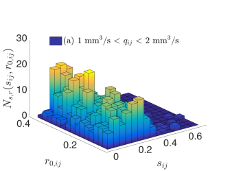
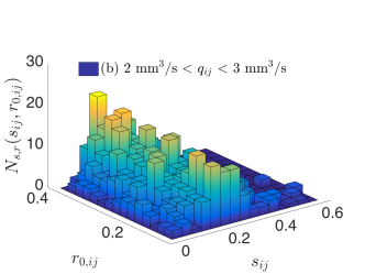
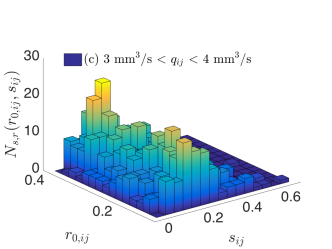
In equation (9) we give the general form of the configurational probability. In Fig. 2, we show histograms $N_{s,r}$ proportional to the joint probability distribution for $s_{ij}$ and $r_{0,ij}$ when only those links fall within a narrow range of volume flows are counted. That is, we record only those links for which (a) 1 mm³/s $<q_{ij}<$ 2 mm³/s, (b)2 mm³/s $<q_{ij}<$ 3 mm³/s, (c) 3 mm³/s $<q_{ij}<$ 4 mm³/s, and (d) 4 mm³/s $<q_{ij}<$ 5 mm³/s. The volume flows $q_{ij}$ ranged roughly between -2.5 mm³/s and 7.5 mm³/s. If equation (10) were true, i.e., $f(x_{b,ij},s_{ij},r_{0,ij})=f(s_{ij},r_{0,ij})$, then the histograms in the four figures should be identical. We see that even though the features are similar, they are not. Hence, there is an $x_{b,ij}$ dependence in $f(x_{b,ij},s_{ij},r_{0,ij})$ for Ca = 0.01.

Figure 3: A cloud plot of $|q_{ij}|$, $s_{ij}$ and $r_{0,ij}$ for Ca = 0.01 and $s=0.5$.

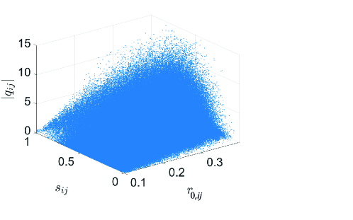
We may transform the distribution in equation (9) from a distribution in $x_{b,ij}$ to a distribution in $|q_{ij}|$,

$$\Pi_{q}(|q_{ij}|,s_{ij},r_{0,ij})=\frac{\langle\left|q\right|\rangle}{\left|q_{ij}\right|}f(x_{b,ij}(|q_{ij}|,s_{ij},r_{0,ij}),s_{ij},r_{0,ij})\ \left[\frac{\partial}{\partial|q_{ij}|}\right]x_{b,ij}(|q_{ij}|,s_{ij},r_{0,ij})\;.$$ (26)

We show in Fig. 3 the cloud of values measured in the system for Ca = 0.01 and $s=0.5$. It is this cloud that equation (26) describes.

Figure 4: Histogram $N_{q}(|q|)$ of volume flow in links when $0.4<s_{ij}<0.5$ and $0.2$ mm $<r_{0,ij}<0.3$ mm for $Ca=0.1$ and (a) $s=0.3$ or (b) $s=0.4$.

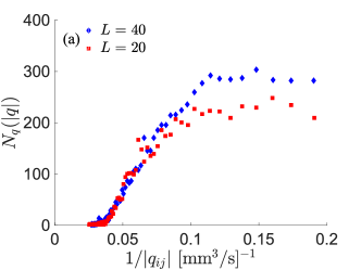
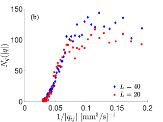
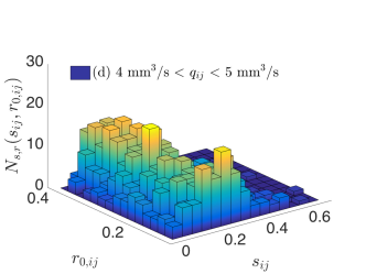
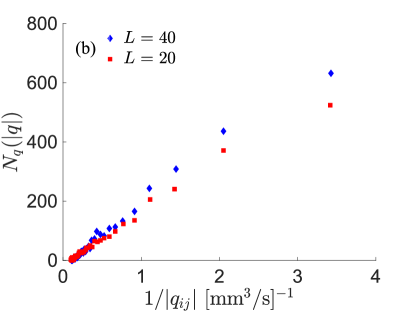
We show in Fig. 4 histograms $N_{q}$ proportional to $\Pi_{q}$ for Ca = 0.1 and for two different system sizes, $L\times L=20\times 20$ and $L\times L=40\times 40$. The volume flows $Q$ have been adjusted so that the capillary numbers are the same for the two system sizes. Only those links with the values of the other two parameters, $s_{ij}$ and $r_{0,ij}$ within a truncated range have been recorded. In Figs. 5 and 6 we show the corresponding histograms for Ca = 0.01. The histograms for Ca = 0.1 show a gap for small values of $1/|q_{ij}|$, and for increasing values of $1/|q_{ij}|$ a somewhat linear region before an essentially flat region occurs. It is not possible from the results for the two system sizes to infer a clear trend that could make it possible to extrapolate the result to infinite system size. The corresponding histograms for the Ca = 0.01 case are in Figs. 5 and 6. They are qualitatively different from the histograms for Ca = 0.1, Fig. 4. There is still a gap for small values of $1/|q_{ij}|$, but from a smallest value, $1/|q_{0,ij}|=1/|\max_{ij}q_{ij}|$, the histogram raises linearly. We also note that the $L=40$ data gives a straighter line that the $L=20$ data. Since the volume flow $Q$ is kept fixed, there is a largest possible link volume flow in the system: $\max_{ij}|q_{ij}|=|Q|$, which would occur if $Q$ in its entirety passed through one link, a possibility that would be more and more likely the smaller the capillary number due to capillary blocking. Hence, for Ca = 0.01, $\Pi_{q}(|q_{ij}|)$ takes the form

$$\Pi_{q}(|q_{ij}|)=g(s_{ij},r_{0,ij})\left[\frac{1}{|q_{ij}|}-\frac{1}{|Q|}\right]\;,$$ (27)

where

$$g(s_{ij},r_{0,ij})=\langle|q|\rangle f(x_{b,ij}(|q_{ij}|,s_{ij},r_{0,ij}),s_{ij},r_{0,ij})\ \left[\frac{\partial}{\partial|q_{ij}|}\right]x_{b,ij}(|q_{ij}|,s_{ij},r_{0,ij})\;.$$ (28)

Figure 5: Histogram $N_{q}(|q|)$ of volume flow in links when $0.3<s_{ij}<0.4$ and $0.2$ mm $<r_{0,ij}<0.3$ mm for $Ca=0.01$ and $s=0.3$.

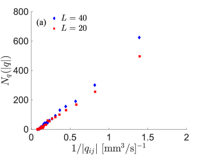
The $|Q|$ dependence in equation (27) comes from the use of the constant-$Q$ ensemble. If each run had been done with $\Delta P$, the pressure drop across the network, kept constant, the $1/|Q|$ term may have vanished. It was shown in Batrouni et al. bhn87 that the choice of ensemble; constant-$Q$ or constant-$\Delta P$ had a profound influence on the high-current end of the current histogram in the random resistor network, a system that shares some similarity to the present one.

It should be noted that the immiscible two-phase flow problem undergoes a phase transition when the saturation is tuned rho09 . For the square lattice, they found the critical saturation to be $s_{c}=a+b\log_{10}\rm Ca$, where $a=0.8$ and $b=0.063$. For Ca = 0.01, this places the critical point at around $s_{c}\approx 0.67$. In analogy with the random resistor network at the percolation threshold, we expect $\Pi_{q}(|q_{ij}|)$ to have a much more complex form than suggested in equation (28) arc85 ; bhl96 , namely that of a multifractal. This has recently been suggested in connection with immiscible two-phase counterflow in porous media zjgz14 .

Figure 6: Histogram $N_{q}(|q|)$ of volume flow in links when $0.4<s_{ij}<0.5$ and $0.2$ mm $<r_{0,ij}<0.3$ mm for $Ca=0.01$ and $s=0.5$.

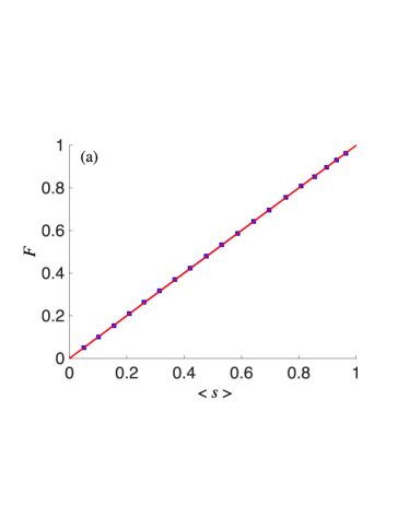
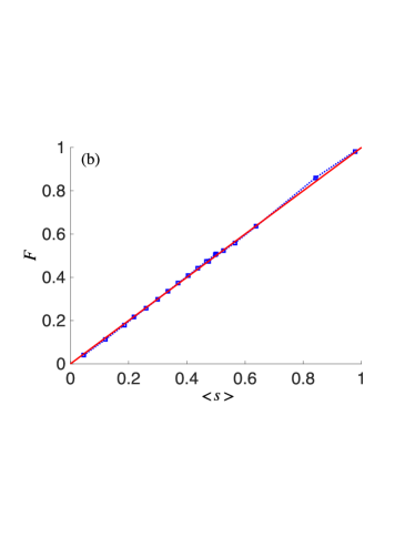
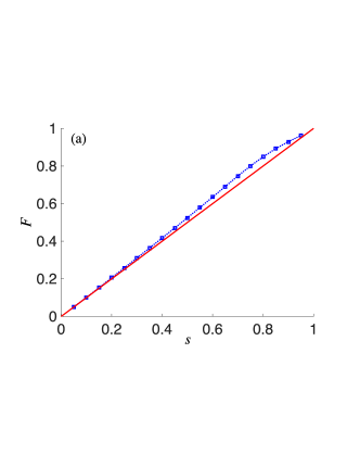
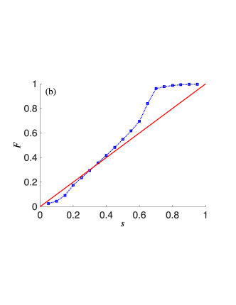
In section IV it was shown that $F=\langle s\rangle$, equation (16), even if capillary forces are important. We demonstrate the validity of this calculation in Fig. 7. In Fig. 8 we show $F$ as a function of volume-weighted average of the saturation $s$. As expected, we see that $F$ is a non-trivial function of $s$. However, for larger capillary numbers, $F$ is closer to the diagonal compared to smaller capillary numbers: compare Fig. 8a with 8b.

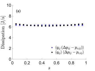
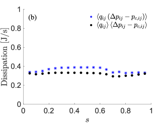
Lastly, we check equation (24) in section IV.4 in Fig. 9. That is, we plot $\langle q_{ij}(\Delta p_{ij}-p_{c,ij})\rangle$ and $\langle|q_{ij}|\rangle\langle|(\Delta p_{ij}-p_{c,ij})|\rangle$ as a function of the saturation $s$. The prediction of equation (24) is that the two quantities should be the same. For Ca=0.1 (Fig. 9a), this works well. For the smaller capillary number Ca=0.01 (Fig. 9b), they match to within some 15% or better.

Figure 7: The non-wetting fractional flow defined in equation (16) $F$ vs. the saturation averaged over the links, $\langle s\rangle$ for (a) Ca = 0.1 and (b) Ca = 0.01. According to this equation, we expect $F=\langle s\rangle$. This is also what we observe.

Figure 8: The non-wetting fractional flow defined in equation (16) $F$ vs. the volume averaged saturation $s$ defined in equation (17) for (a) Ca = 0.1 and (b) Ca = 0.01.

Figure 9: The dissipation $\langle q_{ij}(\Delta p_{ij}-p_{c,ij})\rangle$ and $\langle|q|\rangle\langle|\Delta p-p_{c,ij}|\rangle$ plotted against the non-wetting saturation for (a) Ca =0.1 and (b) Ca = 0.01. Equation (24) predicts that the two data sets should be equal.

VI Conclusion and Perspective

We have presented a statistical mechanical analysis of immiscible two-phase flow in porous media through the introduction and analysis of the ensemble distribution $\Pi(x_{b,ij},s_{ij},r_{0,ij})$ which gives the joint probability density between center-of-mass position of the bubbles, the saturation and the radius of any link in the network that models the porous medium. With the ensemble distribution, any quantity that does not require the relative positions of the links to be taken into account may be calculated. We have presented a few examples in section IV, among them the fractional flow, the average saturation, the average pressure difference leading to the effective mobility, and lastly the entropy production or dissipation. Questions that cannot be answered within this approach are e.g., the relative statistical weight of a given configuration of interfaces within the system which e.g. comes up in connection with the construction of the Markov chain Monte Carlo for sampling fluid configurations. For such questions, the configurational probability density is necessarysshbkv16 .

The ensemble distribution $\Pi(x_{b,ij},s_{ij},r_{0,ij})$ introduced here relates the dynamics of the system to a probability distribution that does not contain time. This is possible due to the ergodicity of the system, see section III. However, since the probability distribution does not contain time, it cannot answer questions that have to do with time explicity, e.g., questions concerning correlation time is outside the realm of this approach.

The ensemble distribution may be transformed into the link volume flow distribution $\Pi_{q}(|q_{ij}|,s_{ij},r_{0,ij})$. This has a surprisingly simple form for moderate capillary numbers, see equation (27). This probability distribution is a close relative of the current distribution function in the random resistor network that was extensively studied and shown to be multifractal in the eighties arc85 ; bhl96 . We expect to find similar complications in the present system when the saturation is at the critical point studied by Ramstad et al. rho09 .

Appendix A Network Model

We use the network model shown in Fig. 1 amhb98 ; kah02 to test some of the central ideas presented in this work. The links represent cylindrical tubes of varying average radii, containing the volume of both the pores and the pore throats of the porous medium. Each link is hour-glass shaped so that the capillary pressure due to an interface at position $0\leq x\leq l$ in the link given by

$$|p_{c,ij}(x)|=\frac{2\gamma\cos\theta}{r_{0}}\left[1-\cos\left(\frac{2\pi x}{l}\right)\right]\;,$$ (29)

where $\gamma$ is the surface tension. The volume flow in each link is related to the pressure difference across it by the Washburn equation

$$q_{ij}=-\frac{\pi r_{0,ij}^{4}}{8\mu_{av,ij}}(\Delta p_{ij}-p_{c,ij})\;,$$ (30)

$\Delta p_{ij}$ is the pressure difference across the link and $p_{c,ij}$ is the sum of the capillary pressure contribution from all the interfaces in the link. For a link with a single bubble with center-of-mass position $x_{b,ij}$ and saturation $s_{ij}$, and surface tension $\gamma$, the capillary pressure on the bubble is given by shbk13

$$p_{c,ij}(x_{b,ij},s_{ij},r_{0,ij})=\frac{4\gamma}{r_{0,ij}}\sin(\pi s_{ij})\sin(\frac{2\pi x_{b,ij}}{l})\;,$$ (31)

At each node volume flow is conserved. This implies that the sum of the contributions from equation (30) are conserved at the nodes. This results in a matrix equation for the pressure field. After solving this equation we can use equation (30) to calculate the flow in each link. From the flow, we can calculate the velocity $u_{ij}=q_{ij}/\pi r_{0,ij}^{2}$ of the fluids. We then move every bubble an amount $\Delta x_{ij}=u_{ij}\Delta t$, where the time step $\Delta t$ is chosen such that no bubble moves more than 10% of the link length.

When the fluid reaches the end of a link, it is redistributed into connected links in proportion to the local flow. If at any given point there are more than three bubbles present in a link, the closest two are merged such that the center of mass of the merged bubbles is conserved. Further details can be found in amhb98 ; kah02 .

References

- (1) J. Bear, Dynamics of fluids in porous media (Dover, Mineola, 1988).
- (2) Wyckoff, R.D. and Botset, H. G., J. of Appl. Phys. 7, 325 (1936).
- (3) J. S. Osoba, J. G. Richardson, J. K. Kerver, J. A. Hafford and P. M. Blair, Petr. Trans. AIME, 192, 47 (1951).
- (4) R. G. Larson, L. E. Scriven and H. T. Davis, Chem. Eng. Sci. 36, 57 (1981).
- (5) W. G. Gray, Int. J. Multiphase Flow, 15, 81 (1989).
- (6) S. M. Hassanizadeh and W. G. Gray, Adv. Wat. Res. 13, 169 (1990).
- (7) S. M. Hassanizadeh and W. G. Grey, Adv. Wat. Res. 16, 53 (1993).
- (8) S. M. Hassanizadeh and W. G. Grey, Wat. Res. Res. 29, 3389 (1993).
- (9) W. G. Gray and S. M. Hassanizadeh, Adv. Wat. Res. 21, 261 (1998).
- (10) R. Hilfer, Phys. Rev. E, 58, 2090 (1998).
- (11) W. G. Gray, Adv. Wat. Res. 22, 521 (1999).
- (12) R. Hilfer and H. Besserer, Physica B, 279, 125 (2000).
- (13) R. Hilfer, Physica A, 359, 119 (2006).
- (14) R. Hilfer, Phys. Rev. E, 73, 016307 (2006).
- (15) R. Hilfer, Physica A, 371, 209 (2006).
- (16) A. Hansen and T. Ramstad, Comp. Geosci. 13, 227 (2009).
- (17) R. Hilfer and F. Döster, Transp. Por. Med. 82, 507 (2010).
- (18) J. Niessner, S. Berg and S. M. Hassanizadeh, Transp. Por. Med. 88, 133 (2011).
- (19) F. Döster, O. Hönig and R. Hilfer, Phys. Rev. E, 86, 016317 (2012).
- (20) R. Hilfer, R. T. Armstrong, S. Berg, A. Georgiadis and H. Ott, Phys. Rev. E, 92, 063023 (2015).
- (21) S. M. Hassanizadeh in Handbook of Porous Media, 3rd edition, edited by K. Vafai (CRC Press, Boca Raton, 2015).
- (22) M. S. Valavanides and T. Daras, Entropy, 18, 54 (2016).
- (23) B. Ghanbarian, M. Sahimi and H. Daigle, Water Res. Res. 52, 5025 (2016).
- (24) A. Hansen, S. Sinha, D. Bedeaux, S. Kjelstrup, I. Savani and M. Vassvik, arXiv:1605.02874 (2016).
- (25) M. J. Blunt, B. Bijeljic, H. Dong, H. Gharbi, S. Iglauer, P. Mostaghimi, A. Paluzny and C. Pentland, Adv. Water Res., 51, 197 (2013).
- (26) S. Bryant and M. J. Blunt, Phys. Rev. A, 46, 2004 (1992).
- (27) E. Aker, K. J. Måløy, A. Hansen and G. G. Batrouni, Transp. Por. Med. 32, 163 (1998).
- (28) H. A. Knudsen, E. Aker and A. Hansen, Transp. Por. Med. 47, 99 (2002).
- (29) G. Tørå, P. E. Øren and A. Hansen, Transp. Por. Med. 92, 145 (2012).
- (30) I. Savani, S. Sinha, D. Bedeaux, S. Kjelstrup and M. Vassvik, arXiv:1606.09339; to appear in Transp. Por. Med.
- (31) V. Joekar-Niasar and S. M. Hassanizadeh, Crit. Rev. in Env. Sci. and Tech. 42, 1895 (2012).
- (32) T. Ramstad, P. E. Øren and S. Bakke, SPE J. 15, 917 (2010).
- (33) T. Ramstad, N. Idowu, C. Nardi and P. E. Øren, Transp. Por. Media, 94, 487 (2012).
- (34) S. Berg, M. Rücker, H. Ott, A. Georgiadis, H. van der Linde, F. Ensmann, M. Kersten, R. T. Armstrong, S. de With, J. Becker and A. Wiegmann, Adv. Wat. Res. 90, 24 (2016).
- (35) R. T. Armstrong, J. E. McClure, M. A. Berrill, M. Rücker, S. Schlüter and S. Berg, Phys. Rev. E, 94, 043113 (2016).
- (36) A. M. Tartakovsky and P. Meakin, J. Comp. Phys. 207, 610 (2005).
- (37) S. Ovaysi and M. Piri, J. Comp. Phys. 229, 7456 (2010).
- (38) M. B. Liu and G. R. Liu, Arch. Comp. Meth. Eng. 17, 25 (2010).
- (39) R. T. Armstrong, S. Berg, O. Dinariev, N. Evseev, D. Klemin, D. Koroteev and S. Safanov, Transp. Por. Med. 112, 577 (2016).
- (40) S. Kjelstrup and D. Bedeaux, Non-Equilibrium Thermodynamics of Heterogeneous Systems (World Scientific, Singapore, 2008).
- (41) S. Kjelstrup, D. Bedeaux, E. Johannesen and J. Gross, Non-Equilibrium Thermodynamics for Engineers, (World Scientific, Singapore, 2010).
- (42) E. C. Childs and N. Collis-George, Proc. Roy. Soc. London, 201, 392 (1950).
- (43) A. E. Scheidegger, J. Appl. Phys. 25, 994 (1954).
- (44) A. E. Scheidegger, Trans. Soc. Rheol. 9, 313 (1965).
- (45) R. H. Aranow, Phys. Fluids, 9, 1721 (1966).
- (46) S. Sinha, A. Hansen, D. Bedeaux and S. Kjelstrup, Phys. Rev. E, 87, 025001 (2013).
- (47) S. Bakke and P. E. Øren. SPE Journal 2, 136 (1997). (2003).
- (48) M. Sahimi, Flow and Transport in Porous Media and Fractured rock, 2nd ed. (Wiley-VCH, Wentheim, 2011).
- (49) M. Erpelding, S. Sinha, K. T. Tallakstad, A. Hansen, E. G. Flekkøy and K. J. Måløy, Phys. Rev. E, 88, 053004 (2013).
- (50) T. Ramstad, A. Hansen and P. E. Øren, Phys. Rev E, 79, 036310 (2009).
- (51) G. G. Batrouni, A. Hansen and M. Nelkin, J. Physique, 48, 771 (1987).
- (52) L. de Arcangelis, S. Redner and A. Coniglio, Phys. Rev. B, 31, 4725 (1985).
- (53) G. G. Batrouni, A. Hansen and B. Larson, Phys. Rev. E, 53, 2292 (1996).
- (54) L. Zhu, N. Jin, Z. Gao and Y. Zong, Petr. Sci. 11, 111 (2014).