A Dipole on the Sky : Predictions for Hypervelocity Stars from the Large Magellanic Cloud
Abstract
We predict the distribution of hypervelocity stars (HVSs) ejected from the Large Magellanic Cloud (LMC), under the assumption that the dwarf galaxy hosts a central massive black hole (MBH). For the majority of stars ejected from the LMC the orbital velocity of the LMC has contributed a significant fraction of their galactic rest frame velocity, leading to a dipole density distribution on the sky. We quantify the dipole using spherical harmonic analysis and contrast with the monopole expected for HVSs ejected from the Galactic Center (GC). There is a tendril in the density distribution that leads the LMC which is coincident with the well-known and unexplained clustering of HVSs in the constellations of Leo and Sextans. Our model is falsifiable, since it predicts that Gaia will reveal a large density of HVSs in the southern hemisphere.
1. Introduction
A hypervelocity star (HVS) is any star whose velocity in the galactic rest frame exceeds the local escape speed of the Milky Way (MW). Several routes have been suggested for their production, the first being reported by Hills (1988) who theorised that the tidal disruption of a stellar binary during a close encounter with the massive black hole (MBH) at the centre of the MW could accelerate one member of the binary, in what is now known as the Hills mechanism.
The first candidate HVS, a B-type star travelling with a galactic rest frame velocity of , was discovered by Brown et al. (2005). Subsequent surveys have discovered dozens of further candidates. The recent review paper Brown (2015) gives a summary, whilst there are subsequent papers by Theissen & West (2014); Savcheva et al. (2014); Hawkins et al. (2015); Kunder et al. (2015); Li et al. (2015); Vickers et al. (2015); Favia et al. (2015). It was noticed early on that the candidate HVSs exhibited significant spatial anisotropy on the sky with 8 out of the 14 HVSs at that time being located in two constellations despite a fifth of the sky having been surveyed (Brown et al., 2009b).
It is a natural extension of the Hills mechanism to ask where else it may occur. For instance Lu et al. (2007) and Sherwin et al. (2008) suggest the central MBHs of M31 and M32 as possible sites. The recent discovery of a red supergiant runaway candidate of M31 by Evans & Massey (2015) suggests these two possibilities may soon be testable. The Large Magellanic Cloud (LMC) is the most massive of the MW’s dwarf satellites and thus there is the potential for the LMC to host a central MBH. The Hills mechanism could accelerate large numbers of stars to a few above the escape speed from the LMC. The LMC has an orbital velocity of (van der Marel & Kallivayalil, 2014), thus alignment of these velocity vectors could result in HVSs that have been ejected from the LMC and are travelling at the escape speed of the MW. The location of the LMC on the sky and orientation of its velocity vector could explain the spatial anisotropy in the observed HVSs.
2. Method
To test the hypothesis that there is a significant number of HVSs ejected from the LMC, we require a prediction for the observables of such a population and a reference population of HVSs from the Galactic Center (GC). We consider three models; HVGC is a model that produces stars from the GC and is identical to HV3 from Kenyon et al. (2014), HVLMC-A is a population from the LMC, and HVLMC-B is identical to HVLMC-A but has the initial ejection velocity cut by to approximate the escape velocity from the centre of the LMC. All three models consider HVSs, which have a typical main sequence lifetime of , since there is a large sample of B-type stars in the HVS literature we can compare to (Brown, 2015). We simulate the process of ejection from the centre of the LMC by seeding HVSs along the orbit of the LMC over the past , with a velocity which is the sum of the orbital velocity of the LMC and the ejection velocity due to the Hills mechanism. These stars are then evolved through a potential model of the MW until a randomly selected observation time, at which point we record the position and velocity in the galactic rest frame. To allow for cross-comparisons with Kenyon et al. (2014), we assume that the Sun is at a position relative to the GC where , and is travelling with a velocity where .
2.1. LMC black hole mass
Observations of dwarf galaxy hosts of MBHs have recently been carried out by Reines et al. (2013), who specifically reference these galaxies as being in the mass range of the LMC. For dwarf galaxies with stellar masses in the range they find MBH masses of , with a median of . Since the dependence of the mean of the ejection velocity from the Hills mechanism is only weakly dependent on the MBH mass (), see Section 2.2, a factor of 10 in MBH mass is only a factor of in the mean ejection velocity. Using Equation 2.2 from Section 2.2, we see that the mean ejection velocity for the binaries with a separation of is , thus MBHs which are times less massive are still capable of ejecting HVSs at velocities of . We thus assume a fiducial value , similar to the median of Reines et al. (2013).
2.2. Hills mechanism
We first require the initial positions and velocities of the candidate HVSs in a frame co-moving with the MBH from which they were ejected. This section uses the prescription of Kenyon et al. (2014), itself based on the Hills mechanism algorithm of Bromley et al. (2006), which we briefly describe here to aid clarity. At the time of their ejection the stars are uniformly distributed across the surface of a sphere with radius centered on the MBH and given an initial outwardly radial trajectory. Thus the only free parameters not yet determined are the magnitude of the velocity , the age of the star when it is ejected , and the age of the star when it is observed .
Suppose that an equal mass binary with separation interacts at a closest approach with a MBH of mass . One star of the system will be ejected by the Hills mechanism with probability
| (1) |
where
| (2) |
The probability that a star is ejected is drawn from a uniform distribution between 0 and 1. If the star is ejected, then following Kenyon et al. (2014), the velocity is drawn from the distribution
| (3) |
where and is given by
| (4) |
We only consider equal mass binaries so . Note that is a normalisation factor (Kenyon et al., 2014)
| (5) |
Since we are interested in all possible equal mass binary systems that can result in an ejection we sample from distributions of and . The separation of the binary is drawn from
| (6) |
where for stars of mass and . The closest approach has
| (7) |
where and .
Both the age of the star at the time of ejection and observation are drawn from the uniform distribution
| (8) |
where and and the main sequence lifetime for stars of mass . The time of flight of the star from ejection to observation is then defined by .
We discard any sampled star that does not satisfy , and . Note that is chosen to minimise the computation time spent on stars that will be difficult to observe. For the HVGC model this corresponds to stars that will remain in the GC so . For stars in the HVLMC-A and HVLMC-B models, we choose to ensure we only include stars that escape the LMC.
2.3. Large Magellanic Cloud orbit
For stars ejected from the centre of the MW, the position and velocity vectors in the galactic rest frame satisfy and . However, for stars ejected from the LMC
| (9) |
where and are the position and velocity vectors of the LMC years ago.
These definitions require knowledge of the position and velocity of the LMC over the past , for which we use an orbit of the LMC around the MW taken from Jethwa et al. (2016), who rewound the orbit of the LMC from the present position including the effect of dynamical friction. The potential used by Jethwa et al. (2016) for the MW is an Navarro, Frenk & White (1996, hereafter NFW) halo with mass and concentration and a Miyamoto & Nagai (1975) disk with radial scale-length and vertical scale-length and a mass chosen to give the solar circular velocity at the position of the sun. The LMC has an NFW halo with mass and concentration and a Plummer bulge with scale-length and a mass chosen to satisfy the mass constraint of van der Marel & Kallivayalil (2014).
2.4. Milky Way potential
For the MW, we use the potential from Kenyon et al. (2008), which was optimised to reproduce the galactic potential at both parsec scales near the MBH Sgr A∗ and at scales of tens of kiloparsecs in the halo. This potential consists of four components
| (10) |
where
| (11) |
is the Keplerian potential of the central MBH with ,
| (12) |
is the Hernquist (1990) potential of the bulge with and ,
| (13) |
is the Miyamoto-Nagai potential of the disk with , and , and
| (14) |
is the NFW potential of the dark matter halo with and . The values for each parameter are from Kenyon et al. (2014).
3. Discussion
3.1. All sky density plots
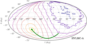
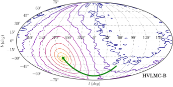
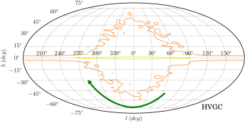
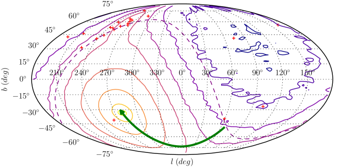
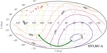
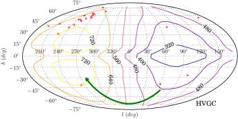
The density distribution of HVSs can be illustrated by an all-sky plot in galactic coordinates, using the equal-area Mollweide projection. We consider only stars with heliocentric distance , since the distance of the LMC is (van der Marel & Kallivayalil, 2014) and this range covers the well-known clustering of HVSs near the constellations of Leo and Sextans reported by Brown et al. (2009b), however the kinematics in the distance bin are broadly similar. Figure 2 suggests that the expected distribution of LMC HVSs on the sky is a dipole, which contrasts with the monopole shown by HVSs from the GC. Note that for the HVGC model the first few contours aren’t shown, since there are HVSs from the GC in our population across the entire sky.
We emphasise that the density contours are not normalised to the ejection rate from either MBH. Brown (2015) justifies an ejection rate of for the MW MBH, but the ejection rate from a MBH at the centre of the LMC will depend significantly on the internal dynamics and star formation rate of the LMC as well as the mass of the MBH. We postpone these considerations to a companion paper, but speculate that the large contribution of the orbital velocity makes an observable signal of LMC HVSs plausible.
In the discovery paper of HVS11, Brown et al. (2009a) commented that that star was within of the Sextans dwarf galaxy while the typical angular separation of HVSs from Local Group dwarf galaxies is . Brown et al. (2009a) ruled out an association with Sextans based on the relative velocity of HVS11 towards Sextans, however the initial instinct that coincidence on the sky is a requirement for association is challenged by Figure 2. The LMC HVSs are distributed across a wide region of the sky.
Figure 1 highlights an intriguing extension of the distribution that leads the LMC and is coincident with the clump observed by Brown et al. (2009b). This is the only area of the sky which is both densely populated in our LMC HVSs models and well-covered by HVS surveys, since almost all of these surveys have covered solely the northern hemisphere, partially due to the footprint of SDSS. The one HVS plotted in Figure 1 that lies in the southern celestial hemisphere is HE 0437-5439 which was discovered by Edelmann et al. (2005), who noted that the flight time was longer than the main sequence lifetime for the star and hence either it is a blue straggler and was ejected as a binary from the GC or has its origin in the LMC.
Brown et al. (2009b) discusses previous attempts to explain the anisotropy, including selection effects, contamination by runaway companions to supernovae, tidal debris from disruption of a dwarf galaxy, temporary intermediate mass black hole companions to the central MBH of the MW, and interactions between two stellar discs near the central MBH which imprint their geometry on the ejected HVSs. Brown (2015) states that the anisotropy is still unexplained and that it will require a southern hemisphere survey to resolve the issue.
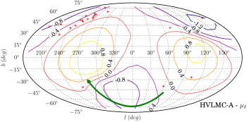
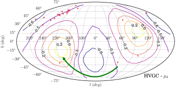
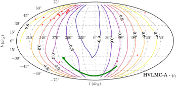
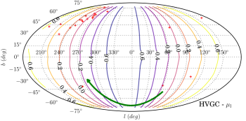
3.2. All sky velocity plots
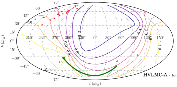
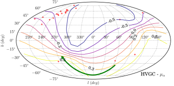
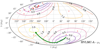
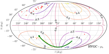
In Figure 3 we show contours of the mean heliocentric radial velocity in each bin, where the standard deviation in each plot is a couple . The remaining two velocity dimensions are summarised in Figure 4, where we plot contours of the mean proper motion in each bin in both equatorial and galactic coordinates with a typical standard deviation of . For the HVLMC-A model the contours demonstrate the imprint of the orbital velocity of the LMC in the kinematics of the HVSs, while for the HVGC stars the dominant effect is the solar rotation.
Considering Figures 3 and 4, we see that at the locations on the sky of the currently observed B-type HVSs the velocity distributions of HVSs in the HVGC and HVLMC-A models are coincident. Since each model has a standard deviation of and the current proper motions for these stars have a typical error of (Brown et al., 2015), it will not be possible to test our hypothesis using the current sample of HVSs. This situation should be resolved by Gaia, which will give proper motions for HVSs in regions on the sky where the two models differ by up to . To illustrate this point, the first and third quartile ranges of the magnitude of the proper motions for stars at a distance are in the HVGC model and in the HVLMC-A model. Comparing these ranges to end-of-mission proper motion errors for Gaia111 http://www.cosmos.esa.int/web/gaia/science-performance of around for B1V stars with apparent magnitude , corresponding to stars at about , it may be possible for Gaia to distinguish between the two populations.
3.3. Spherical harmonics
One method of quantifying the relative spatial distributions of HVSs from the centre of the galaxy and the LMC is to consider the power in each mode of the spherical harmonic power spectrum of the density. For spherical harmonics defined by
| (15) |
where and are the colatidudinal and longitudinal coordinates, we can expand any function that is square-integrable on the unit sphere as
| (16) |
Using the orthonormality property of our chosen definition of the spherical harmonics we can then write
| (17) |
For our purposes, the function is a sum of delta functions on the unit sphere at the locations of each of the HVSs:
| (18) |
Noting that , this sum of delta functions transforms Equation 17 into a sum over the HVSs,
| (19) |
The angular power spectrum of is then given by
| (20) |
and are plotted for our populations of HVSs in Figure 5.
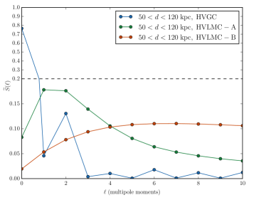
Almost all of the power for the HVGC stars in this distance range is in the monopole, which we expect as the highest velocity stars are ejected along essentially straight lines from the GC, and at the difference between the the observer being located at the sun or the GC is minimal. The HVLMC-A model has a peak in power in the dipole/quadrupole, with a long tail that is caused by the fast stars ejected ahead of the LMC and slow stars lagging behind. The distinguishing features between the two models are
-
1.
a strong monopole in the HVGC model versus a strong dipole/quadrupole in the HVLMC-A model,
-
2.
a large amount of power at high in the HVLMC-A model.
The HVLMC-B model has a large section of the sky where there are no HVSs, thus is not well-approximated by a dipole. The power is then spread across a large number of modes since no one mode is a good approximation. With the upcoming first data release of Gaia we may soon be in a position to use spherical harmonic analysis to distinguish between production mechanisms of HVSs.
4. Conclusions
Hypervelocity stars (HVSs) created in the Large Magellanic Cloud (LMC) may contribute in a significant way to the sky distribution. This may provide a natural solution to the clustering of HVSs in the direction of Leo and Sextans found by Brown et al. (2009b). Uniquely, this area of the sky is densely populated by LMC origin models and is well-covered by current HVS surveys.
This hypothesis can shortly be tested by surveys in the southern celestial hemisphere, such as SkyMapper and Gaia. If these surveys fail to find a significant number of HVSs near the LMC, the model will be falsified. A possible reason for failure is that the LMC does not host a significant black hole. However, our choice of the Hills mechanism as the production route was solely due to its proposed dominance in the MW (Brown, 2015). Other production routes which will be active in the disk of the LMC, such as runaway companions of supernovae and three-body dynamical interactions, can still result in high-velocity stars. Since the orbital velocity of the LMC can provide (van der Marel & Kallivayalil, 2014), stars from these two mechanisms only need to be ejected at the escape velocity of the LMC () to be considered anonymously high velocity stars. The sky distributions of these populations are under investigation in a companion paper.
The HVS candidate SDSS J121150.27+143716.2 was recently shown to be a binary by Németh et al. (2016), who concluded that the usual production routes for HVSs cannot achieve a galactic rest frame velocity of without disrupting the binary and thus the binary is either an extreme halo object or was accreted from the debris of a destroyed satellite galaxy. While the kinematics of this candidate are inconsistent with the LMC, we speculate that the addition of the orbital velocity of a Local Group dwarf galaxy with the ejection velocity due to a standard HVS production route could explain this HVS binary.
SkyMapper and Gaia will increase the quantity and quality of our HVS sample across the entire sky and thus enable more sophisticated analysis techniques, including our proposed spherical harmonic analysis, which is capable of distinguishing between hypervelocity populations in a quantitative way. Coincidence on the sky is not a necessary requirement for association with a Local Group dwarf galaxy. The satellites of the MW may well have imprinted distinctive signatures on the distribution of HVSs right across the sky.
Acknowledgements
DB thanks the STFC for a studentship. The orbit integration utilised galpy (Bovy, 2015). We thank Prashin Jethwa for the use of his LMC orbit and Scott Kenyon for useful and prompt answers to our queries. We further acknowledge the anonymous referee for comments that improved the clarity of our results.
References
- Bovy (2015) Bovy, J. 2015, ApJS, 216, 29
- Bromley et al. (2006) Bromley, B. C., Kenyon, S. J., Geller, M. J., et al. 2006, ApJ, 653, 1194
- Brown (2015) Brown, W. R. 2015, ARA&A, 53, 15
- Brown et al. (2015) Brown, W. R., Anderson, J., Gnedin, O. Y., et al. 2015, ApJ, 804, 49
- Brown et al. (2009a) Brown, W. R., Geller, M. J., & Kenyon, S. J. 2009a, ApJ, 690, 1639
- Brown et al. (2009b) Brown, W. R., Geller, M. J., Kenyon, S. J., & Bromley, B. C. 2009b, ApJL, 690, L69
- Brown et al. (2005) Brown, W. R., Geller, M. J., Kenyon, S. J., & Kurtz, M. J. 2005, ApJL, 622, L33
- Edelmann et al. (2005) Edelmann, H., Napiwotzki, R., Heber, U., Christlieb, N., & Reimers, D. 2005, ApJL, 634, L181
- Evans & Massey (2015) Evans, K. A., & Massey, P. 2015, AJ, 150, 149
- Favia et al. (2015) Favia, A., West, A. A., & Theissen, C. A. 2015, ApJ, 813, 26
- Hawkins et al. (2015) Hawkins, K., Kordopatis, G., Gilmore, G., et al. 2015, MNRAS, 447, 2046
- Hills (1988) Hills, J. G. 1988, Nature, 331, 687
- Jethwa et al. (2016) Jethwa, P., Erkal, D., & Belokurov, V. 2016, arXiv:1603.04420
- Kenyon et al. (2014) Kenyon, S. J., Bromley, B. C., Brown, W. R., & Geller, M. J. 2014, ApJ, 793, 122
- Kenyon et al. (2008) Kenyon, S. J., Bromley, B. C., Geller, M. J., & Brown, W. R. 2008, ApJ, 680, 312
- Kunder et al. (2015) Kunder, A., Rich, R. M., Hawkins, K., et al. 2015, ApJL, 808, L12
- Li et al. (2015) Li, Y.-B., Luo, A.-L., Zhao, G., et al. 2015, RAA, 15, 1364
- Lu et al. (2007) Lu, Y., Yu, Q., & Lin, D. N. C. 2007, ApJL, 666, L89
- Németh et al. (2016) Németh, P., Ziegerer, E., Irrgang, A., et al. 2016, ApJL, 821, L13, arXiv: 1604.03158
- Reines et al. (2013) Reines, A. E., Greene, J. E., & Geha, M. 2013, ApJ, 775, 116
- Savcheva et al. (2014) Savcheva, A. S., West, A. A., & Bochanski, J. J. 2014, ApJ, 794, 145
- Sherwin et al. (2008) Sherwin, B. D., Loeb, A., & O’Leary, R. M. 2008, MNRAS, 386, 1179
- Theissen & West (2014) Theissen, C. A., & West, A. A. 2014, ApJ, 794, 146
- van der Marel & Kallivayalil (2014) van der Marel, R. P., & Kallivayalil, N. 2014, ApJ, 781, 121
- Vickers et al. (2015) Vickers, J. J., Smith, M. C., & Grebel, E. K. 2015, AJ, 150, 77