The forecasting of menstruation based on a state-space
modeling of basal body temperature time series

Abstract

Women’s basal body temperature (BBT) follows a periodic pattern that is associated with the events in their menstrual cycle. Although daily BBT time series contain potentially useful information for estimating the underlying menstrual phase and for predicting the length of current menstrual cycle, few models have been constructed for BBT time series. Here, we propose a state-space model that includes menstrual phase as a latent state variable to explain fluctuations in BBT and menstrual cycle length. Conditional distributions for the menstrual phase were obtained by using sequential Bayesian filtering techniques. A predictive distribution for the upcoming onset of menstruation was then derived based on the conditional distributions and the model, leading to a novel statistical framework that provided a sequentially updated prediction of the day of onset of menstruation. We applied this framework to a real dataset comprising women’s self-reported BBT and days of menstruation, comparing the prediction accuracy of our proposed method with that of conventional calendar calculation. We found that our proposed method provided a better prediction of the day of onset of menstruation. Potential extensions of this framework may provide the basis of modeling and predicting other events that are associated with the menstrual cycle.

Key words: Basal body temperature, Menstrual cycle length, Periodic phenomena, Sequential prediction, State-space model, Time series analysis.

Introduction

The menstrual cycle is the periodic changes that occur in the female reproductive system that make pregnancy possible. Throughout the menstrual cycle, basal body temperature (BBT) also follows a periodic pattern. The menstrual cycle consists of two phases, the follicular phase followed by the luteal phase, with ovulation occurring at the transition between the two phases. During the follicular phase, BBT is relatively low with the nadir occurring within 1 to 2 days of a surge in luteinizing hormone that triggers ovulation. After the nadir, the cycle enters the luteal phase and BBT rises by $0.3$ to $0.5\ {}^{\circ}\mathrm{C}$ (Barron and Fehring 2005).

Considerable attention has been paid to the development of methods to predict the days of ovulation and the day of onset of menstruation; currently available methods include urinary and plasma hormone analyses, ultrasound monitoring of follicular growth, and monitoring of changes in the cervical mucus or BBT. Monitoring the change in BBT is straightforward because it requires neither expensive instruments nor medical expertise. However, of the currently available methods, BBT measurement is the least reliable because it has an inherently large day-to-day variability (Barron and Fehring 2005); therefore, statistical analyses are required to improve predictions of events associated with the menstrual cycle based on BBT.

Many statistical models of the menstrual cycle have been proposed, with the majority explaining the marginal distribution of menstrual cycle length which is characterized by a long right tail. To explain within-individual heterogeneity, which is an important source of variation in menstrual cycle length, Harlow and Zeger (1991) made the biological assumption that a single menstrual cycle is composed of a period of “waiting” followed by the ovarian cycle. They classified menstrual cycles into standard, normally distributed cycles that contained no waiting time and into nonstandard cycles that contained waiting time. Guo et al. (2006) extended this idea and proposed a mixture model consisting of a normal distribution and a shifted Weibull distribution to explain the right-tailed distribution. By accommodating covariates, they also investigated the effect of an individual’s age on the moments of the cycle length distribution. Huang et al. (2014) attempted to model the changes in the mean and variance of menstrual cycle length that occur during the approach of menopause. By using a change-point model, they found changes in the annual rate of change of the mean and variance of menstrual cycle length which indicate the start of early and late menopausal transition. In contrast, Bortot et al. (2010) focused on the dynamic aspect of menstrual cycle length over time. By using a state-space modeling approach, they derived a predictive distribution of menstrual cycle length that was conditional on past time series. By integrating a fecundability model into their time series model, they also developed a framework that estimates the probability of conception that is conditional on the within-cycle intercourse behavior. A related joint modeling of menstrual cycle length and fecundity has been attained more recently (Lum et al. 2016).

Although daily fluctuations in BBT are associated with the events of the menstrual cycle, and therefore BBT time series analyses likely provide information regarding the length of the current menstrual cycle, there have been no previous studies modeling BBT data to predict menstrual cycle length. Thus, in the present study we developed a statistical framework that provides a predictive distribution of menstrual cycle length (which, by extension, is a predictive distribution of the next day of onset of menstruation) that is sequentially updated with daily BBT data. We used a state-space model that includes a latent phase state variable to explain daily fluctuations in BBT and to derive a predictive distribution of menstrual cycle length that is dependent on the current phase state.

This paper is organized as follows: In Section 2, we briefly describe the data required for the proposed method and how the test dataset was obtained. In Section 3, we provide the formulation of the proposed state-space model for menstrual cycle and give an overview of the filtering algorithms that we use to estimate the conditional distributions of the latent phase variable given the model and dataset. In the same section, we also describe the predictive probability distribution for the next day of onset of menstruation that was derived from the proposed model and the filtering distribution for the menstrual phase. In Section 4, we apply the proposed framework to a real dataset and compare the accuracy of the point prediction of the next day of onset of menstruation between the proposed method and the conventional method of calendar calculation. In Section 5, we discuss the practical utility of the proposed method with respect to the management of women’s health and examine the potential challenges and prospects for the proposed framework.

Data

We assumed that for a given female subject a dataset containing a daily BBT time series and days of onset of menstruation was available. The BBT could be measured with any device (e.g., a conventional thermometer or a wearable sensor), although different model parameters may be adequate for different measurement devices. In the application of the proposed framework described in Section 4, we used real BBT time series and menstruation onset data that was collected via a website called Ran’s story (QOL Corporation, Ueda, Japan), which is a website that allows registered users to upload their self-reported daily BBT and days of menstruation onset to QOL Corporation’s data servers. At the time of registering to use the service, all users of Ran’s story agree to the use of their data for academic research. Although no data regarding the ethnic characteristics of the users were available, it is assumed that the majority, if not all, the users were ethnically Japanese because Ran’s story is provided only in the Japanese language.

Model description and inferences

State-space model of the menstrual cycle

Here we develop a state-space model for a time series of observed BBT, $y_{t}$, and an indicator of the onset of menstruation, $z_{t}$, obtained for a subject for days $t=1,\dots,T$. By $z_{t}=1$, we denote that menstruation started on day $t$, whereas $z_{t}=0$ indicates that day $t$ is not the first day of menstruation. We denote the BBT time series and menstruation data obtained until time $t$ as $Y_{t}=(y_{1},\dots,y_{t})$ and $Z_{t}=(z_{1},\dots,z_{t})$, respectively.

We considered the phase of the menstrual cycle, $\theta_{t}\in\mathbb{R}~{}(t=0,1,\dots,T)$, to be a latent state variable. We let $\epsilon_{t}$ as the daily advance of the phase and assume that it is a positive random variable that follows a gamma distribution with shape parameter $\alpha$ and rate parameter $\beta$, which leads to the following system model:

$$\theta_{t}=\theta_{t-1}+\epsilon_{t}$$ (1)

$$\epsilon_{t}\sim\textrm{Gamma}(\alpha,\beta).$$ (2)

Under this assumption, the conditional distribution of $\theta_{t}$, given $\theta_{t-1}$, is a gamma distribution with a probability density function:

$$p(\theta_{t}\mid\theta_{t-1})=\textrm{Gamma}(\alpha,\beta)$$

$$=\frac{\beta^{\alpha}}{\Gamma(\alpha)}(\theta_{t}-\theta_{t-1})^{\alpha-1}\exp\left\{-\beta(\theta_{t}-\theta_{t-1})\right\}.$$ (3)

It is assumed that the distribution for the observed BBT $y_{t}$ is conditional on the phase $\theta_{t}$. Since periodic oscillation throughout each phase is expected for BBT, a finite trigonometric series is used to model the average BBT. Assuming a Gaussian observation error, the observation model for BBT is expressed as

$$y_{t} =a+\sum_{m=1}^{M}(b_{m}\cos 2m\pi\theta_{t}+c_{m}\sin 2m\pi\theta_{t})+e_{t}\hskip 20.00003pt$$ (4)

$$e_{t} \sim\textrm{Normal}(0,\sigma^{2}),$$ (5)

where $M$ is the maximum order of the series. Conditional on $\theta_{t}$, $y_{t}$ then follows a normal distribution with a probability density function:

$$p(y_{t}\mid\theta_{t}) =\textrm{Normal}\left\{\mu(\theta_{t}),\sigma^{2}\right\}$$

$$=\frac{1}{\sqrt{2\pi\sigma^{2}}}\exp\left[-\frac{\left\{y_{t}-\mu(\theta_{t})\right\}^{2}}{2\sigma^{2}}\right],$$ (6)

where $\mu(\theta_{t})=a+\sum_{m=1}^{M}(b_{m}\cos 2m\pi\theta_{t}+c_{m}\sin 2m\pi\theta_{t})$. By this definition, $\mu(\theta_{t})$ is periodic in terms of $\theta_{t}$ with a period of 1.

For the onset of menstruation, we assume that menstruation starts when $\theta_{t}$ “steps over” the smallest following integer. This is represented as follows:

$$z_{t} =0\hskip 20.00003pt\textrm{when}\hskip 20.00003pt\lfloor\theta_{t}\rfloor=\lfloor\theta_{t-1}\rfloor$$ (7)

$$=1\hskip 20.00003pt\textrm{when}\hskip 20.00003pt\lfloor\theta_{t}\rfloor>\lfloor\theta_{t-1}\rfloor,$$ (8)

where $\lfloor x\rfloor$ is the floor function that returns the largest previous integer for $x$. Writing this deterministic allocation in a probabilistic manner, which is conditional on $(\theta_{t},\theta_{t-1})$, $z_{t}$ follows a Bernoulli distribution:

$$p(z_{t}\mid\theta_{t},\theta_{t-1})$$

$$=(1-z_{t})\left\{I(\lfloor\theta_{t}\rfloor=\lfloor\theta_{t-1}\rfloor)\right\}+z_{t}\left\{I(\lfloor\theta_{t}\rfloor>\lfloor\theta_{t-1}\rfloor)\right\},$$ (9)

where $I(x)$ is the indicator function that returns 1 when $x$ is true or 0 otherwise.

Let $\boldsymbol{\xi}=(\alpha,\beta,\sigma,a,b_{1},\dots,b_{M},c_{1},\dots c_{M})$ be a vector of the parameters of this model. Given a time series of BBT, $Y_{T}=(y_{1},\dots,y_{T})$, an indicator of menstruation, $Z_{T}=(z_{1},\dots,z_{T})$, and a distribution specified for initial states, $p(\theta_{1},\theta_{0})$, these parameters can be estimated by using the maximum likelihood method. The log-likelihood of this model is expressed as

$$l(\boldsymbol{\xi};Y_{T},Z_{T})$$

$$=\log p(y_{1},z_{1}\mid\boldsymbol{\xi})+\sum_{t=2}^{T}\log p(y_{t},z_{t}\mid Y_{t-1},Z_{t-1},\boldsymbol{\xi}),$$ (10)

where

$$\log p(y_{1},z_{1}\mid\boldsymbol{\xi})$$

$$=\log\int\int p(y_{1}\mid\theta_{1})p(z_{1}\mid\theta_{1},\theta_{0})p(\theta_{1},\theta_{0})d\theta_{1}d\theta_{0},$$ (11)

and for $t=2,\dots,T$,

$$\log p(y_{t},z_{t}\mid Y_{t-1},Z_{t-1},\boldsymbol{\xi})$$

$$=\log\int\int p(y_{t}\mid\theta_{t})p(z_{t}\mid\theta_{t},\theta_{t-1})$$

$$\hskip 50.00008pt\times p(\theta_{t},\theta_{t-1}\mid Y_{t-1},Z_{t-1})d\theta_{t}d\theta_{t-1},$$ (12)

which can be sequentially obtained by using the Bayesian filtering technique described below. Note that although $p(y_{t}\mid\theta_{t})(t\geq 1)$ and $p(\theta_{t},\theta_{t-1}\mid Y_{t-1},Z_{t-1})(t\geq 2)$ depend on $\boldsymbol{\xi}$, this dependence is not explicitly described for notational simplicity.

State estimation and calculation of log-likelihood by using the non-Gaussian filter

Given the state-space model of menstrual cycle described above and its parameters and data, the conditional distribution of an unobserved menstrual phase can be obtained by using recursive formulae for the state estimation problem, which are referred to as the Bayesian filtering and smoothing equations (Särkkä 2013). We describe three versions of this sequential procedure, that is, prediction, filtering, and smoothing, for the state-space model described above.

Let $p(\theta_{t},\theta_{t-1}\mid Y_{t},Z_{t})$ be the joint distribution for the phase at successive time points $t-1$ and $t$, which is conditional on the observations obtained by time $t$. This conditional distribution accommodates all the data obtained by time $t$ and is called the filtering distribution. Similarly, the joint distribution for the phase of successive time points $t$ and $t-1$ conditional on the observations obtained by time $t-1$, $p(\theta_{t},\theta_{t-1}\mid Y_{t-1},Z_{t-1})$, is referred to as the one-step-ahead predictive distribution. For $t=1,\dots,T$ these distributions are obtained by sequentially applying the following recursive formulae:

$$p(\theta_{t},\theta_{t-1}\mid Y_{t-1},Z_{t-1})$$

$$=p(\theta_{t}\mid\theta_{t-1})p(\theta_{t-1}\mid Y_{t-1},Z_{t-1})$$

$$=p(\theta_{t}\mid\theta_{t-1})\int p(\theta_{t-1},\theta_{t-2}\mid Y_{t-1},Z_{t-1})d\theta_{t-2}$$ (13)

$$p(\theta_{t},\theta_{t-1}\mid Y_{t},Z_{t})$$

$$=\frac{p(y_{t},z_{t}\mid\theta_{t},\theta_{t-1})p(\theta_{t},\theta_{t-1}\mid Y_{t-1},Z_{t-1})}{\int\int p(y_{t},z_{t}\mid\theta_{t},\theta_{t-1})p(\theta_{t},\theta_{t-1}\mid Y_{t-1},Z_{t-1})d\theta_{t}d\theta_{t-1}}$$

$$=\frac{p(y_{t}\mid\theta_{t})p(z_{t}\mid\theta_{t},\theta_{t-1})p(\theta_{t},\theta_{t-1}\mid Y_{t-1},Z_{t-1})}{\int\int p(y_{t}\mid\theta_{t})p(z_{t}\mid\theta_{t},\theta_{t-1})p(\theta_{t},\theta_{t-1}\mid Y_{t-1},Z_{t-1})d\theta_{t}d\theta_{t-1}}$$ (14)

where for $t=1$ we set $p(\theta_{1},\theta_{0}\mid Y_{0},Z_{0})$ as $p(\theta_{1},\theta_{0})$, which is the specified initial distribution for the phase. Equations (13) and (14) are the prediction and filtering equation, respectively. Note that the denominator in Equation (14) is the likelihood for data at time $t$ (see Equations 11 and 12). Hence, the log-likelihood of the state-space model is obtained through application of the Bayesian filtering procedure.

The joint distribution for the phase, which is conditional on the entire set of observations, $p(\theta_{t},\theta_{t-1}\mid Y_{T},Z_{T})$, is referred to as the (fixed-interval type) smoothed distribution. With the filtering and the one-step-ahead predictive distributions, the smoothed distribution is obtained by recursively using the following smoothing formula:

$$p(\theta_{t},\theta_{t-1}\mid Y_{T},Z_{T})$$

$$=p(\theta_{t},\theta_{t-1}\mid Y_{t},Z_{t})\int\frac{p(\theta_{t+1},\theta_{t}\mid Y_{T},Z_{T})p(\theta_{t+1}\mid\theta_{t})}{p(\theta_{t+1},\theta_{t}\mid Y_{t},Z_{t})}d\theta_{t+1}$$

$$=\frac{p(\theta_{t},\theta_{t-1}\mid Y_{t},Z_{t})\int p(\theta_{t+1},\theta_{t}\mid Y_{T},Z_{T})d\theta_{t+1}}{p(\theta_{t}\mid Y_{t},Z_{t})}$$

$$=\frac{p(\theta_{t},\theta_{t-1}\mid Y_{t},Z_{t})\int p(\theta_{t+1},\theta_{t}\mid Y_{T},Z_{T})d\theta_{t+1}}{\int p(\theta_{t},\theta_{t-1}\mid Y_{t},Z_{t})d\theta_{t-1}}.$$ (15)

In general, these recursive formulae are not analytically tractable for non-linear, non-Gaussian, state-space models. However, the conditional distributions, as well as the log-likelihood of the state-space model, can still be approximated by using filtering algorithms for general state-space models. We use Kitagawa’s non-Gaussian filter (Kitagawa 1987) where the continuous state space is discretized into equally spaced grid points at which the probability density is evaluated. We describe the numerical procedure to obtain these conditional distributions by using the non-Gaussian filter in Appendix A.

Predictive distribution for the day of onset of menstruation

A predictive distribution for the day of onset of menstruation is derived from the assumptions of the model and the filtering distribution of the state.

We denote the distribution function and the probability density function of the gamma distribution with shape parameter $s$ and rate parameter $r$ as $G(\hskip 1.00006pt\cdot\hskip 1.00006pt;s,r)$ and $g(\hskip 1.00006pt\cdot\hskip 1.00006pt;s,r)$, respectively. Let the accumulated advance of the phase be denoted by $\Delta_{k}(t)$, which is then calculated as $\Delta_{k}(t)=\sum_{r=t+1}^{t+k}\epsilon_{r},k=1,2,\cdots$. We consider the conditional probability that the next menstruation has occurred before day $k+t$ given the phase state $\theta_{t}$. We denote this conditional probability as $F(k\mid\theta_{t})=\textrm{Pr}\left\{\Delta_{k}(t)>\lceil\theta_{t}\rceil-\theta_{t}\right\}$, where $\lceil x\rceil$ is the ceiling function that returns the smallest following integer for $x$. Therefore, $F(k\mid\theta_{t})$ represents the conditional distribution function for the onset of menstruation. Under the assumption of the state-space model described above, $F(k\mid\theta_{t})$ is given as

$$F(k\mid\theta_{t}) =\int_{\lceil\theta_{t}\rceil-\theta_{t}}^{\infty}g(x;k\alpha,\beta)dx$$

$$=1-G(\lceil\theta_{t}\rceil-\theta_{t};k\alpha,\beta).$$ (16)

The conditional probability function for the day of onset of menstruation, denoted as $f(k\mid\theta_{t})$, is then given as

$$f(k\mid\theta_{t})$$

$$=F(k\mid\theta_{t})-F(k-1\mid\theta_{t})$$

$$=\left\{1-G(\lceil\theta_{t}\rceil-\theta_{t};k\alpha,\beta)\right\}$$

$$\hskip 40.00006pt-\left[1-G\left\{\lceil\theta_{t}\rceil-\theta_{t};(k-1)\alpha,\beta\right\}\right]$$

$$=G\left\{\lceil\theta_{t}\rceil-\theta_{t};(k-1)\alpha,\beta\right\}-G(\lceil\theta_{t}\rceil-\theta_{t};k\alpha,\beta),$$ (17)

where we set $F(0\mid\theta_{t})=0$.

The marginal distribution for the day of onset of menstruation, denoted as $h(k\mid Y_{t},Z_{t})$, can also be obtained with the marginal filtering distribution for the phase state, $p(\theta_{t}\mid Y_{t},Z_{t})$. It is given as

$$h(k\mid Y_{t},Z_{t})=\int f(k\mid\theta_{t})p(\theta_{t}\mid Y_{t},Z_{t})d\theta_{t}.$$ (18)

Note that this distribution is conditional on the data obtained by time $t$ and therefore provides a predictive distribution for menstruation day that accommodates all information available. The point prediction for menstruation day can also be obtained from $h(k\mid Y_{t},Z_{t})$ and one of the natural choice for it would be the $k$ that gives the highest probability, $\max h(k\mid Y_{t},Z_{t})$.

Table 1: Summary of self-reported menstrual cycle data obtained from 10 subjects.

	Subject
	1	2	3	4	5	6	7	8	9	10
All data
No. of consecutive cycles	47	46	49	55	53	58	57	53	46	45
Range of cycle length	[28, 59]	[23, 45]	[19, 61]	[26, 59]	[18, 47]	[25, 49]	[25, 36]	[26, 56]	[30, 51]	[27, 48]
Mean of cycle length	39.4	33.2	32.8	31.2	27.2	29.7	30.1	31.7	34.1	33.4
Median of cycle length	38	33	32.5	30.5	26	29	30	31	32	33
SD of cycle length	6.7	4.1	5.6	4.7	4.9	3.9	2.6	5.2	4.7	4.6
Initial age	29.6	24.9	23.2	26.3	30.5	33.2	34.9	29.9	33.9	31.4
Final age	34.5	29.0	27.6	30.9	34.4	37.8	39.5	34.4	38.1	35.4
Length of time series	1812	1495	1576	1687	1418	1693	1687	1647	1534	1470
No. of missing observations	80	0	96	31	43	33	21	85	38	60
Data for parameter estimation
No. of consecutive cycles	29	29	29	29	29	29	29	29	29	29
Range of cycle length	[31, 59]	[23, 43]	[19, 39]	[26, 59]	[22, 37]	[25, 49]	[27, 36]	[26, 56]	[30, 51]	[27, 42]
Mean of cycle length	41.3	33.7	31.5	30.6	26.7	30.4	30.9	33.0	34.7	32.1
Median of cycle length	41	34	32	29	26	30	31	32	32	31
SD of cycle length	7.2	4.0	3.9	5.8	3.3	4.8	2.5	5.9	5.8	3.5
Length of time series	1199	978	914	888	776	882	897	958	1007	933
No. of missing observations	24	0	52	21	20	22	8	5	19	34
Data for predictive accuracy estimation
No. of consecutive cycles	18	17	20	26	24	29	28	24	17	16
Range of cycle length	[28, 44]	[28, 45]	[26, 61]	[28, 39]	[18, 47]	[26, 36]	[25, 36]	[26, 39]	[31, 35]	[27, 48]
Mean of cycle length	36.1	32.3	34.8	32.0	27.9	29.0	29.3	30.0	32.9	35.8
Median of cycle length	35	32	33	32	27	28	30	29	33	35
SD of cycle length	4.2	4.2	7.2	2.7	6.5	2.5	2.5	3.6	1.4	5.6
Length of time series	613	517	662	799	642	811	790	689	527	537
No. of missing observations	56	0	44	10	23	11	13	80	19	26

We describe the non-Gaussian filter-based numerical procedure we used to obtain these predictive distributions in Appendix A.

Application

We used the BBT time series and menstruation onset data provided by 10 users of the Ran’s story website (QOL Corporation, Ueda, Japan). Data were collected through the course of 44 to 57 consecutive menstrual cycles (see Table 1 for a summary of the data). Data of each subject’s first 29 consecutive menstrual cycles were used to fit the state-space model described above and to obtain maximum likelihood estimates of the parameters. To determine the order of the trigonometric series, models with $M=1,2,\dots,12$ (referring to models M1, M2, …, and M12, respectively) were fitted and then compared based on the Akaike information criterion (AIC) for each subject. The best AIC model and the remaining menstrual cycle data (i.e., the data that were not used for the parameter estimations), were then used to evaluate the accuracy of the prediction of the next day of onset of menstruation based on the root mean square error (RMSE) and the mean absolute error (MAE) for each subject. We compared the prediction accuracy between the sequential prediction and the conventional, fixed prediction, where the former was obtained by using the proposed method and the latter was obtained as the day after a fixed number of days from the onset of preceding menstruation.

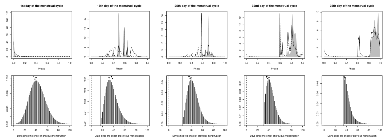
Figure 2: Example estimated conditional distributions for menstrual phase (upper panels) and the associated predictive distributions for the day of onset of menstruation (lower panels). In the upper panels, predictive and filtering distributions are shown as dashed and solid lines, respectively, and smoothed distributions are represented by gray shading. $x$-axes represent $\theta_{t}\mod 1$. In the lower panels, the marginal probabilities of the onset of menstruation $h(k\mid Y_{t},Z_{t})$ are shown. Dashed and solid vertical lines indicate the day of onset of the previous menstruation and the current day, respectively. Filled circles indicate the actual day of onset of the next menstruation. Filled and open triangles indicate the best conventional prediction for the subject and the model-based prediction, respectively. These results were obtained by applying the best AIC model to the first menstrual cycle of the test data of subject 1. From left to right, panels correspond to 21, 14, 7, and 3 days before the upcoming day of onset of menstruation, respectively.

Parameter estimates in the best AIC model for the 10 subjects are shown in Table 2. The selected order of the trigonometric series ranged from 5 to 12. The estimated relationship between expected BBT and menstrual phase, and the estimated probability density distribution for phase advancement for each subject are shown in Figure 1. Although the estimated temperature-phase regression lines were “squiggly” due to the high order of the trigonometric series, they in general exhibited two distinct stages: the temperature tended to be lower in the first half of the cycle and higher in the second half, which is consistent with the well-known periodicity of BBT through the menstrual cycle (Barron and Fehring 2005). Figure 2 shows examples of the estimated conditional distributions for menstrual phase and the associated predictive distributions for the day of onset of menstruation.

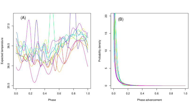
Figure 1: Model components for each subject. Each color represents a different subject. Lines show the best AIC model associated with the maximum likelihood estimates for each subject. (A) Relationship between expected temperature and menstrual phase. The $x$-axis represents $\theta_{t}\mod 1$. (B) Probability density distribution for the advancement per day of the menstrual phase.

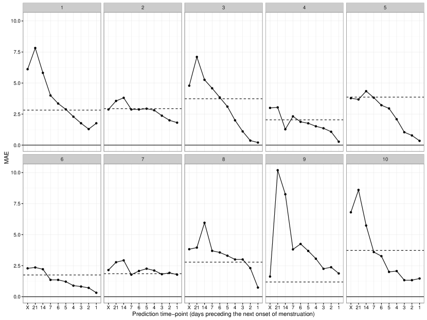
Figure 4: Mean absolute error (MAE) of the prediction of the day of onset of the next menstruation. Solid lines indicate the MAE of the sequential prediction (based on the best AIC model for each subject), and horizontal dashed lines indicate the lowest MAE of the conventional prediction for each subject. On the horizontal axis, “X” indicates the prediction obtained at the day of onset of the previous menstruation. Each panel shows the results for one subject. Compared with the best prediction provided by the conventional method, the range, mean and median of the rate of the maximum reduction of MAE for each subject by using the sequential method was 0.056–1.368, 0.449 and 0.311, respectively.

The RMSE of the predictions of the next day of onset of menstruation provided by the sequential method and by the conventional method are shown in Figure 3 (see Tables 3 and 4 in Appendix B for more details). In the sequential method, the RMSE tended to decrease as the day approached the next day of onset of menstruation, suggesting that accumulation of the BBT time series data contributed to increasing the accuracy of the prediction. Although, at the day of onset of preceding menstruation, the sequential method does not necessarily provide a more accurate prediction compared with the conventional method, it may provide a much-improved prediction as the day gets closer to the onset of next menstruation. Except for in subject 9, the sequential method exhibited a better predictive performance than the conventional method for at least one of the time points of prediction we considered (i.e., the day preceding the next day of onset of menstruation) (Figure 3). Compared with the best prediction provided by the conventional method, the range, mean, and median of the rate of the maximum reduction in the RMSE for each subject in the sequential method was 0.066–1.481, 0.557 and 0.487, respectively. Note that the predictive performance tended to be even better when the accuracy was measured by using the mean absolute error (see Tables 5 and 6 and Figure 4 in Appendix B).

Table 2: Results of fitting the state-space model by using the maximum likelihood method. Parameter estimates and their 95% confidence intervals (in brackets) of the best AIC model are shown for each subject. Log-likelihood was approximated by using the non-Gaussian filter with the state-space was discretized with 512 intervals.

	Subject
	1	2	3	4	5	6	7	8	9	10
Best model	M10	M8	M9	M6	M11	M8	M11	M12	M10	M5
$\alpha$	0.210	0.953	0.344	1.520	0.318	1.971	0.630	0.172	0.150	0.201
	$[0.151,0.292]$	$[0.628,1.439]$	$[0.253,0.467]$	$[1.015,2.266]$	$[0.233,0.435]$	$[1.329,2.905]$	$[0.449,0.882]$	$[0.128,0.231]$	$[0.106,0.211]$	$[0.140,0.288]$
$\beta$	8.915	32.131	10.916	45.146	8.536	59.929	19.510	5.886	5.284	6.544
	$[6.303,12.610]$	$[21.157,48.798]$	$[7.883,15.115]$	$[30.420,67.002]$	$[6.094,11.955]$	$[40.536,88.601]$	$[13.806,27.572]$	$[4.236,8.178]$	$[3.595,7.766]$	$[4.429,9.669]$
$\sigma$	0.112	0.161	0.119	0.121	0.093	0.152	0.108	0.101	0.116	0.209
	$[0.103,0.121]$	$[0.150,0.173]$	$[0.109,0.130]$	$[0.113,0.129]$	$[0.085,0.102]$	$[0.142,0.163]$	$[0.098,0.120]$	$[0.094,0.109]$	$[0.109,0.123]$	$[0.195,0.224]$
$a$	36.299	36.203	36.485	36.384	36.632	36.522	36.518	36.519	36.645	36.123
	$[36.247,36.351]$	$[36.187,36.219]$	$[36.466,36.504]$	$[36.370,36.397]$	$[36.614,36.650]$	$[36.509,36.535]$	$[36.501,36.536]$	$[36.492,36.546]$	$[36.620,36.670]$	$[36.087,36.160]$
$b_{1}$	0.193	0.197	0.174	0.098	$-0.034$	0.107	0.130	0.141	0.129	0.138
	$[0.153,0.232]$	$[0.179,0.216]$	$[0.147,0.200]$	$[0.074,0.122]$	$[-0.072,0.003]$	$[0.088,0.126]$	$[0.101,0.159]$	$[0.114,0.169]$	$[0.099,0.159]$	$[0.082,0.193]$
$b_{2}$	0.015	0.024	$-0.028$	$-0.079$	0.115	$-0.063$	$-0.001$	$-0.370$	$-0.012$	0.002
	$[-0.021,0.050]$	$[-0.010,0.058]$	$[-0.061,0.006]$	$[-0.096,-0.061]$	$[0.063,0.167]$	$[-0.081,-0.046]$	$[-0.024,0.022]$	$[-0.416,-0.323]$	$[-0.067,0.043]$	$[-0.082,0.085]$
$b_{3}$	0.009	$-0.057$	0.027	0.032	$-0.098$	0.018	0.025	$-0.089$	$-0.087$	$-0.126$
	$[-0.112,0.130]$	$[-0.085,-0.029]$	$[-0.001,0.056]$	$[0.012,0.051]$	$[-0.148,-0.048]$	$[-0.003,0.039]$	$[0.001,0.049]$	$[-0.132,-0.045]$	$[-0.136,-0.038]$	$[-0.192,-0.060]$
$b_{4}$	$-0.039$	0.021	$-0.023$	0.007	0.124	$-0.028$	$-0.032$	0.167	$-0.078$	$-0.153$
	$[-0.075,-0.003]$	$[-0.010,0.053]$	$[-0.051,0.005]$	$[-0.017,0.030]$	$[0.094,0.153]$	$[-0.054,-0.001]$	$[-0.061,-0.003]$	$[0.105,0.229]$	$[-0.125,-0.030]$	$[-0.250,-0.056]$
$b_{5}$	0.058	$-0.046$	0.013	$-0.020$	$-0.129$	$-0.030$	0.029	0.174	0.049	$-0.003$
	$[-0.006,0.121]$	$[-0.097,0.005]$	$[-0.028,0.054]$	$[-0.039,-0.002]$	$[-0.165,-0.092]$	$[-0.061,0.000]$	$[0.001,0.057]$	$[0.137,0.212]$	$[-0.040,0.139]$	$[-0.153,0.148]$
$b_{6}$	$-0.014$	0.046	$-0.065$	$-0.022$	0.097	0.028	$-0.001$	$-0.038$	0.100	NA
	$[-0.230,0.202]$	$[-0.005,0.098]$	$[-0.106,-0.024]$	$[-0.051,0.006]$	$[0.045,0.149]$	$[-0.001,0.058]$	$[-0.030,0.029]$	$[-0.122,0.047]$	$[0.040,0.160]$
$b_{7}$	$-0.024$	0.019	0.006	NA	$-0.078$	$-0.026$	0.024	$-0.112$	$-0.003$	NA
	$[-0.485,0.437]$	$[-0.030,0.068]$	$[-0.034,0.046]$		$[-0.124,-0.032]$	$[-0.068,0.016]$	$[-0.015,0.062]$	$[-0.149,-0.075]$	$[-0.104,0.099]$
$b_{8}$	0.037	0.034	$-0.063$	NA	0.088	0.037	0.060	$-0.098$	$-0.058$	NA
	$[-0.256,0.331]$	$[-0.037,0.105]$	$[-0.145,0.020]$		$[0.047,0.129]$	$[-0.011,0.085]$	$[0.011,0.109]$	$[-0.180,-0.017]$	$[-0.171,0.056]$
$b_{9}$	$-0.086$	NA	$-0.045$	NA	$-0.060$	NA	0.007	0.010	$-0.036$	NA
	$[-0.231,0.060]$		$[-0.142,0.051]$		$[-0.090,-0.029]$		$[-0.019,0.033]$	$[-0.033,0.053]$	$[-0.136,0.064]$
$b_{10}$	0.061	NA	NA	NA	0.101	NA	0.050	0.120	0.053	NA
	$[-0.170,0.293]$				$[0.062,0.140]$		$[0.002,0.097]$	$[0.062,0.178]$	$[-0.036,0.141]$
$b_{11}$	NA	NA	NA	NA	$-0.058$	NA	0.031	0.023	NA	NA
					$[-0.100,-0.016]$		$[-0.032,0.094]$	$[-0.023,0.069]$
$b_{12}$	NA	NA	NA	NA	NA	NA	NA	$-0.114$	NA	NA
								$[-0.145,-0.082]$
$c_{1}$	$-0.193$	$-0.108$	$-0.182$	$-0.270$	$-0.184$	$-0.170$	$-0.254$	$-0.417$	$-0.172$	$-0.276$
	$[-0.304,-0.081]$	$[-0.140,-0.075]$	$[-0.218,-0.146]$	$[-0.289,-0.252]$	$[-0.204,-0.164]$	$[-0.190,-0.150]$	$[-0.274,-0.233]$	$[-0.463,-0.371]$	$[-0.218,-0.126]$	$[-0.334,-0.217]$
$c_{2}$	$-0.051$	$-0.131$	$-0.130$	$-0.034$	$-0.107$	$-0.058$	$-0.038$	$-0.216$	$-0.035$	$-0.057$
	$[-0.085,-0.018]$	$[-0.154,-0.108]$	$[-0.159,-0.101]$	$[-0.058,-0.010]$	$[-0.133,-0.080]$	$[-0.082,-0.035]$	$[-0.059,-0.017]$	$[-0.263,-0.169]$	$[-0.069,-0.001]$	$[-0.107,-0.006]$
$c_{3}$	$-0.089$	$-0.029$	$-0.022$	$-0.056$	0.006	$-0.023$	$-0.021$	0.062	$-0.070$	$-0.019$
	$[-0.120,-0.059]$	$[-0.065,0.008]$	$[-0.051,0.006]$	$[-0.076,-0.037]$	$[-0.041,0.052]$	$[-0.046,-0.000]$	$[-0.044,0.002]$	$[0.018,0.106]$	$[-0.126,-0.014]$	$[-0.096,0.059]$
$c_{4}$	$-0.030$	$-0.001$	$-0.035$	0.005	$-0.016$	$-0.012$	0.016	0.248	$-0.047$	0.042
	$[-0.174,0.114]$	$[-0.042,0.041]$	$[-0.063,-0.007]$	$[-0.014,0.025]$	$[-0.077,0.046]$	$[-0.038,0.014]$	$[-0.013,0.044]$	$[0.202,0.295]$	$[-0.118,0.024]$	$[-0.065,0.148]$
$c_{5}$	$-0.003$	$-0.058$	0.027	$-0.017$	0.010	$-0.037$	$-0.016$	$-0.040$	$-0.082$	$-0.126$
	$[-0.256,0.250]$	$[-0.117,0.001]$	$[-0.007,0.062]$	$[-0.040,0.007]$	$[-0.047,0.067]$	$[-0.067,-0.007]$	$[-0.044,0.011]$	$[-0.099,0.019]$	$[-0.134,-0.029]$	$[-0.186,-0.066]$
$c_{6}$	$-0.053$	$-0.003$	0.023	$-0.034$	$-0.007$	$-0.025$	$-0.010$	$-0.277$	0.004	NA
	$[-0.143,0.037]$	$[-0.055,0.050]$	$[-0.030,0.076]$	$[-0.059,-0.008]$	$[-0.052,0.038]$	$[-0.062,0.013]$	$[-0.036,0.015]$	$[-0.312,-0.243]$	$[-0.107,0.114]$
$c_{7}$	0.068	$-0.030$	$-0.031$	NA	0.010	$-0.040$	$-0.052$	$-0.075$	0.059	NA
	$[-0.040,0.176]$	$[-0.080,0.020]$	$[-0.073,0.012]$		$[-0.038,0.057]$	$[-0.086,0.006]$	$[-0.081,-0.023]$	$[-0.136,-0.015]$	$[0.014,0.104]$
$c_{8}$	$-0.050$	0.044	0.067	NA	$-0.044$	0.027	0.027	0.214	0.074	NA
	$[-0.324,0.223]$	$[-0.002,0.089]$	$[0.006,0.127]$		$[-0.102,0.013]$	$[-0.028,0.082]$	$[-0.014,0.068]$	$[0.171,0.257]$	$[-0.009,0.157]$
$c_{9}$	$-0.027$	NA	$-0.085$	NA	0.006	NA	0.007	0.079	$-0.067$	NA
	$[-0.675,0.620]$		$[-0.134,-0.036]$		$[-0.059,0.071]$		$[-0.049,0.063]$	$[0.036,0.122]$	$[-0.169,0.034]$
$c_{10}$	0.025	NA	NA	NA	$-0.019$	NA	0.013	$-0.107$	$-0.057$	NA
	$[-0.494,0.543]$				$[-0.088,0.050]$		$[-0.032,0.058]$	$[-0.172,-0.041]$	$[-0.156,0.042]$
$c_{11}$	NA	NA	NA	NA	0.041	NA	0.067	$-0.022$	NA	NA
					$[-0.011,0.093]$		$[0.025,0.108]$	$[-0.057,0.014]$
$c_{12}$	NA	NA	NA	NA	NA	NA	NA	0.012	NA	NA
								$[-0.053,0.077]$
log-likelihood	$468.905$	$164.278$	$206.631$	$415.909$	$343.887$	$234.46$	$354.47$	$408.464$	$330.137$	$-178.022$

Discussion

Here we constructed a statistical framework that provides a model-based prediction of the day of onset of menstruation based on a state-space model and an associated Bayesian filtering algorithm. The model describes the daily fluctuation of BBT and the history of menstruation. The filtering algorithms yielded a filtering distribution of menstrual phase that was conditional on all of the data available at that point in time, which was used to derive a predictive distribution for the next day of onset of menstruation.

The predictive framework we developed has several notable characteristics that make it superior to the conventional method of calendar calculation for predicting the day of onset of menstruation. State-space modeling and Bayesian filtering techniques enable the proposed method to yield sequential predictions of the next day of onset of menstruation based on daily BBT data. Even though menstrual cycle length fluctuates stochastically, the prediction of day of onset of menstruation is automatically adjusted based on the daily updated filtering distribution, yielding a flexible yet robust prediction of the next day of onset of menstruation. This is markedly different from the conventional method that yields only a fixed prediction that is never adjusted. In a study similar to the present study, Bortot et al. (2010) constructed a predictive framework for menstrual cycle length by using the state-space modeling approach. However, in their model, the one-step-ahead predictive distribution for menstrual cycle length is obtained based on the past time series of cycle length and within-cycle information is not taken into account in the prediction.

Furthermore, compared to the conventional method, the proposed sequential method generally yielded a more accurate prediction of day of onset of menstruation. As the day approaches the next onset of menstruation and more daily temperature data are accumulated, the proposed method produced a considerably improved prediction (Figure 3). Since measuring BBT is a simple and inexpensive means of determining the current phase of the menstrual cycle, the proposed framework can provide predictions of the next onset of menstruation that can easily be implemented for the management of women’s health. Although the non-Gaussian filtering technique may be computationally impractical for a state-space model with a high-dimensional state vector (Kitagawa 1987), our proposed model only involves a two-dimensional state vector so the computational cost required for filtering single data is negligible for a contemporary computer.

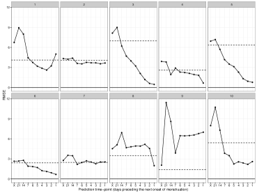
Figure 3: Root mean square error (RMSE) of the prediction of the day of onset of the next menstruation. Solid lines indicate the RMSE of the sequential prediction (based on the best AIC model for each subject), and horizontal dashed lines indicate the lowest RMSE of the conventional prediction for each subject. On the horizontal axis, “X” indicates the prediction obtained at the day of onset of the previous menstruation. Each panel shows the results for one subject.

The conditional probability density distribution for menstrual phase obtained with the sequential Bayesian filter may also be used for predicting other events that are related to the menstrual cycle. For example, the conditional probability of the menstrual phase being below or above a “change point” of expected temperature could be used as a model-based probability of the subject being in the follicular phase (before ovulation) or the luteal phase (after ovulation). These probabilities may also be used to estimate the timing of ovulation. Combined with a fecundability model that provides the probability of conception within a menstrual cycle that is conditional on daily intercourse behavior, the model might also be used to predict the probability of conception (Bortot et al. 2010, Lum et al. 2016). As the Bayesian filtering algorithm can yield predictive and smoothed distributions (Equations 13 and 15), these predictions could be obtained in both a prospective and a retrospective manner. Another possible extension of the model may be the addition of a new observation model for the physical condition of subjects, which may help to estimate the menstrual phase more precisely or to provide a forecast of the physical condition of subject as their menstrual cycle progresses.

We note that the state-space model proposed in the present study may not be sufficiently flexible to describe the full variation in menstrual cycle length. In the present study, we fitted our model only to data from 10 subjects and this data did not include extremely short or extremely long cycles because a preliminary investigation suggested that inclusion of such data could result in unreasonable parameter estimates (results not shown). Specifically, the estimates of $\alpha$ and $\beta$ may become extremely small, leading to an almost flat probability density distribution for menstrual phase advancement. Under these parameter values, the predictive distribution for the onset of menstruation also becomes flat, preventing a useful prediction from being obtained. These results suggest that with a single set of parameter values, the proposed state-space model does not capture the whole observed variation in cycle length. It is known that the statistical distribution of menstrual cycle length is characterized by a mixture distribution that comprises standard and nonstandard cycles, where, for the latter, a skewed distribution may well represent the observed pattern (e.g., Harlow and Zeger 1991, Guo et al. 2006, Lum et al. 2016). Our proposed model, however, does not provide such a mixture-like marginal distribution for the day of onset of menstruation. It is also known that the mean and variance of the marginal distribution of cycle length can vary depending on subjects’ age (Guo et al. 2006, Bortot et al. 2010, Huang et al. 2014). Therefore, we assume that modeling variations in the system model parameters (i.e., $\alpha$ and $\beta$), by including covariates such as age or within- and among-subject random effects, or both, may be a promising extension of the proposed framework. To explain the skewed marginal distribution of menstrual cycle length, Sharpe and Nordheim (1980) considered a rate process in which the development rate fluctuates randomly. Inclusion of random effects for the system model parameters would allow us to accommodate this idea. Although the inclusion of random effects will increase the flexibility of the framework, it would also considerably complicate the likelihood calculation and make parameter estimation more challenging.

The state-space model proposed here provides a conceptual description of the menstrual cycle. We explain this perspective by using the analogy of a clock that makes one complete revolution in each menstrual cycle. The system model expresses the hand of the clock (i.e., the latent phase variable) moving steadily forward with an almost steadily, yet slightly variable, pace. Observation models describe observable events that are imprinted on the clock’s dial; for example, menstruation is scheduled to occur when the hand of this clock arrives at a specific point on the dial. The fluctuation in BBT, as well as other possibly related phenomena such as ovulation, would also be marked on the dial. Even though the position of the hand of the clock is unobservable, we can estimate it as a conditional distribution of the latent phase variable by using the Bayesian filtering technique, which enables us to make a sequential, model-based prediction of menstruation. Although this is a rather phenomenological view of the menstrual cycle, it is useful for developing a rigorous and extendable modeling framework for predicting and studying phenomena that are associated with the menstrual cycle.

Appendix A State estimation, likelihood calculation, and prediction using the non-Gaussian filter

The statistical inferences described in Section 3 of the main text were based on an estimation of the conditional distribution of the latent menstrual phase. Although the conditional distribution can be obtained by using the recursive equations described in Section 3.2, the integrals in those formulae are generally not analytically tractable for non-linear, non-Gaussian, state-space models. Therefore, to obtain approximate conditional distributions, filtering algorithms for general state-space models are required. We use the non-Gaussian filter proposed by Kitagawa (1987), in which the continuous state space is discretized with equally spaced fixed points at which the conditional probability density is evaluated. With these discretized probability density functions, integrals are evaluated by using numerical integration. This filtering algorithm also yields an approximate log-likelihood, making the maximum likelihood estimation of the model parameters possible. Detailed descriptions for this numerical procedure are provided, for example, in Kitagawa (1987, 2010) and de Valpine and Hastings (2002).

To apply non-Gaussian filtering to the state-space model described in Section 3.1, it is computationally more convenient to consider the state space of a circular phase variable rather than a linear phase variable described in the main text, because the latter requires discretization of unbounded real space. Hence, in the following, we first reformulate the statistical modeling framework in terms of a circular latent phase variable. The reformulated model conceptually agrees with the original formulation, given the probability that the menstrual phase advancement per day being more than 1 (i.e., $\mbox{Pr}(\epsilon_{t}>1)$) is negligible. In practice, this condition is naturally attained in the estimation of the model parameters as long as unusually short menstrual cycles (e.g., 3 to 4 days) are not included in the dataset. Below, we provide a numerical procedure to obtain the conditional distributions, log-likelihood, and the predictive distribution of the next day of onset of menstruation based on the non-Gaussian filtering technique (note, all definitions and notations are the same as those used in Section 3 of the main text).

Model with a circular state variable

Instead of using the real latent state variable for the menstrual phase, $\theta_{t}\in\mathbb{R}$, we reformulate the model with a circular latent variable of period 1, denoted by $\omega_{t}\in[0,1)$. We consider that the correspondence between these two variables is characterized by the following projection: $\omega_{t}=f(\theta_{t})=\theta_{t}\mod 1$. The system model for this circular variable is then expressed as

$$\omega_{t}=\left(\omega_{t-1}+\epsilon_{t}\right)\mod 1$$ (19)

$$\epsilon_{t}\sim\textrm{Gamma}(\alpha,\beta).$$ (20)

Under this assumption, given $\omega_{t-1}$, the conditional distribution of $\omega_{t}$ is a wrapped gamma distribution with a probability density function:

$$p(\omega_{t}\mid\omega_{t-1})$$

$$=\textrm{wGamma}(\alpha,\beta)$$

$$=\frac{\beta^{\alpha}}{\Gamma(\alpha)}\exp\left\{-\beta\delta(\omega_{t},\omega_{t-1})\right\}$$

$$\hskip 40.00006pt\times\Phi\left\{\exp(-\beta),1-\alpha,\delta(\omega_{t},\omega_{t-1})\right\},$$ (21)

where $\delta(\omega_{t},\omega_{t-1})=(\omega_{t}-\omega_{t-1})^{I(\omega_{t}>\omega_{t-1})}(1+\omega_{t}-\omega_{t-1})^{I(\omega_{t}\leq\omega_{t-1})}$ is the advancement of the menstrual phase on the circular scale and $\Phi(z,s,a)=\sum_{k=0}^{\infty}\frac{z^{k}}{(a+k)^{s}}$ is Lerch’s transcendental function (Coelho 2007).

The observation model for BBT, which is conditional on $\omega_{t}$, is expressed as

$$y_{t} =a+\sum_{m=1}^{M}(b_{m}\cos 2m\pi\omega_{t}+c_{m}\sin 2m\pi\omega_{t})+e_{t}\hskip 20.00003pt$$ (22)

$$e_{t} \sim\textrm{Normal}(0,\sigma^{2}),$$ (23)

leading to a normal conditional distribution of $y_{t}$ with a probability density function:

$$p(y_{t}\mid\omega_{t}) =\textrm{Normal}\left\{\mu(\omega_{t}),\sigma^{2}\right\}$$

$$=\frac{1}{\sqrt{2\pi\sigma^{2}}}\exp\left[-\frac{\left\{y_{t}-\mu(\omega_{t})\right\}^{2}}{2\sigma^{2}}\right],$$ (24)

where $\mu(\omega_{t})=a+\sum_{m=1}^{M}(b_{m}\cos 2m\pi\omega_{t}+c_{m}\sin 2m\pi\omega_{t})$.

Assuming that $\mbox{Pr}(\epsilon_{t}>1)$ is negligible, we consider menstruation to have started when $\omega_{t}$ “steps over” $1$. This is represented as

$$z_{t} =0\hskip 20.00003pt\textrm{when}\hskip 20.00003pt\omega_{t}>\omega_{t-1}$$ (25)

$$=1\hskip 20.00003pt\textrm{when}\hskip 20.00003pt\omega_{t}\leq\omega_{t-1}.$$ (26)

We can write this deterministic allocation in a probabilistic manner that is conditional on $(\omega_{t},\omega_{t-1})$, where $z_{t}$ follows a Bernoulli distribution:

$$p(z_{t}\mid\omega_{t},\omega_{t-1})=$$

$$(1-z_{t})\left\{I(\omega_{t}>\omega_{t-1})\right\}+z_{t}\left\{I(\omega_{t}\leq\omega_{t-1})\right\}.$$ (27)

The log-likelihood of this model can then be expressed as

$$l(\boldsymbol{\xi};Y_{T},Z_{T})=$$

$$\log p(y_{1},z_{1}\mid\boldsymbol{\xi})+\sum_{t=2}^{T}\log p(y_{t},z_{t}\mid Y_{t-1},Z_{t-1},\boldsymbol{\xi}),$$ (28)

where

$$\log p(y_{1},z_{1}\mid\boldsymbol{\xi})$$

$$=\log\int_{0}^{1}\int_{0}^{1}p(y_{1}\mid\omega_{1})p(z_{1}\mid\omega_{1},\omega_{0})p(\omega_{1},\omega_{0})d\omega_{1}d\omega_{0},$$ (29)

and for $t=2,\dots,T$,

$$\log p(y_{t},z_{t}\mid Y_{t-1},Z_{t-1},\boldsymbol{\xi})$$

$$=\log\int_{0}^{1}\int_{0}^{1}p(y_{t}\mid\omega_{t})p(z_{t}\mid\omega_{t},\omega_{t-1})$$

$$\hskip 40.00006pt\times p(\omega_{t},\omega_{t-1}\mid Y_{t-1},Z_{t-1})d\omega_{t}d\omega_{t-1}.$$ (30)

For $t=1,\dots,T$, the prediction, filtering, and smoothing equations for the above model are expressed as follows:

$$p(\omega_{t},\omega_{t-1}\mid Y_{t-1},Z_{t-1})$$

$$=p(\omega_{t}\mid\omega_{t-1})p(\omega_{t-1}\mid Y_{t-1},Z_{t-1})$$

$$=p(\omega_{t}\mid\omega_{t-1})\int_{0}^{1}p(\omega_{t-1},\omega_{t-2}\mid Y_{t-1},Z_{t-1})d\omega_{t-2}$$ (31)

$$p(\omega_{t},\omega_{t-1}\mid Y_{t},Z_{t})$$

$$=\frac{p(y_{t},z_{t}\mid\omega_{t},\omega_{t-1})p(\omega_{t},\omega_{t-1}\mid Y_{t-1},Z_{t-1})}{\int_{0}^{1}\int_{0}^{1}p(y_{t},z_{t}\mid\omega_{t},\omega_{t-1})p(\omega_{t},\omega_{t-1}\mid Y_{t-1},Z_{t-1})d\omega_{t}d\omega_{t-1}}$$

$$=\frac{p(y_{t}\mid\omega_{t})p(z_{t}\mid\omega_{t},\omega_{t-1})p(\omega_{t},\omega_{t-1}\mid Y_{t-1},Z_{t-1})}{\int_{0}^{1}\int_{0}^{1}p(y_{t}\mid\omega_{t})p(z_{t}\mid\omega_{t},\omega_{t-1})p(\omega_{t},\omega_{t-1}\mid Y_{t-1},Z_{t-1})d\omega_{t}d\omega_{t-1}}$$ (32)

$$p(\omega_{t},\omega_{t-1}\mid Y_{T},Z_{T})$$

$$=p(\omega_{t},\omega_{t-1}\mid Y_{t},Z_{t})\int_{0}^{1}\frac{p(\omega_{t+1},\omega_{t}\mid Y_{T},Z_{T})p(\omega_{t+1}\mid\omega_{t})}{p(\omega_{t+1},\omega_{t}\mid Y_{t},Z_{t})}d\omega_{t+1}$$

$$=\frac{p(\omega_{t},\omega_{t-1}\mid Y_{t},Z_{t})\int_{0}^{1}p(\omega_{t+1},\omega_{t}\mid Y_{T},Z_{T})d\omega_{t+1}}{p(\omega_{t}\mid Y_{t},Z_{t})}$$

$$=\frac{p(\omega_{t},\omega_{t-1}\mid Y_{t},Z_{t})\int_{0}^{1}p(\omega_{t+1},\omega_{t}\mid Y_{T},Z_{T})d\omega_{t+1}}{\int_{0}^{1}p(\omega_{t},\omega_{t-1}\mid Y_{t},Z_{t})d\omega_{t-1}},$$ (33)

where for $t=1$, we set $p(\omega_{1},\omega_{0}\mid Y_{0},Z_{0})$ as $p(\omega_{1},\omega_{0})$, which is the specified initial distribution for the phase.

We consider the conditional probability that the next menstruation has started by day $k+t$, given the phase state $\omega_{t}$, to be $F(k\mid\omega_{t})=\textrm{Pr}\left\{\Delta_{k}(t)>1-\omega_{t}\right\}$. Then, $F(k\mid\omega_{t})$ represents the conditional distribution function for the onset of menstruation, and under the assumption of the state-space model described above, this is given as

$$F(k\mid\omega_{t}) =\int_{1-\omega_{t}}^{\infty}g(x;k\alpha,\beta)dx$$

$$=1-G(1-\omega_{t};k\alpha,\beta).$$ (34)

The conditional probability function for the day of onset of menstruation, $f(k\mid\omega_{t})$, is then given as

$$f(k\mid\omega_{t}) =F(k\mid\omega_{t})-F(k-1\mid\omega_{t})$$

$$=\left\{1-G(1-\omega_{t};k\alpha,\beta)\right\}$$

$$\hskip 40.00006pt-\left[1-G\left\{1-\omega_{t};(k-1)\alpha,\beta\right\}\right]$$

$$=G\left\{1-\omega_{t};(k-1)\alpha,\beta\right\}-G(1-\omega_{t};k\alpha,\beta),$$ (35)

where we set $F(0\mid\omega_{t})=0$.

The marginal distribution for the day of onset of menstruation, $h(k\mid Y_{t},Z_{t})$, is then obtained with the marginal filtering distribution for the phase state, $p(\omega_{t}\mid Y_{t},Z_{t})$, which is given as

$$h(k\mid Y_{t},Z_{t})=\int_{0}^{1}f(k\mid\omega_{t})p(\omega_{t}\mid Y_{t},Z_{t})d\omega_{t},$$ (36)

which is used to provide a point prediction for the day of onset of menstruation by finding the value of $k$ that gives the highest probability, $\max h(k\mid Y_{t},Z_{t})$.

Numerical procedure for non-Gaussian filtering

We let $\omega(i),~{}i=1,\dots,N$ be equally spaced grid points with interval $[0,1)$. We denote the approximate probability density of the predictive, filtering, and smoothed distributions evaluated at these grid points on the state space by $\tilde{p}_{\mbox{p}}(i,j,t),\tilde{p}_{\mbox{f}}(i,j,t)$, and $\tilde{p}_{\mbox{s}}(i,j,t)$, which are defined respectively as

$$\tilde{p}_{\mbox{p}}(i,j,t)=p\left\{\omega_{t}=\omega(i),\omega_{t-1}=\omega(j)\mid Y_{t-1},Z_{t-1}\right\}$$ (37)

$$\tilde{p}_{\mbox{f}}(i,j,t)=p\left\{\omega_{t}=\omega(i),\omega_{t-1}=\omega(j)\mid Y_{t},Z_{t}\right\}$$ (38)

$$\tilde{p}_{\mbox{s}}(i,j,t)=p\left\{\omega_{t}=\omega(i),\omega_{t-1}=\omega(j)\mid Y_{T},Z_{T}\right\},$$ (39)

where for $i,j=1,\dots,N$ and $t=1,\dots,T$. As the initial distribution, we also specify the probability density $\tilde{p}_{\mbox{p}}(i,j,0)$. We define the probability density function of the system model (Equation 21) evaluated at each grid point as $\tilde{p}_{\mbox{m}}(i,j)=p\left\{\omega_{t}=\omega(i)\mid\omega_{t-1}=\omega(j)\right\}$. Then, the prediction, filtering, and smoothing equations, respectively, are expressed as

$$\tilde{p}_{\mbox{p}}(i,j,t)=\tilde{p}_{\mbox{m}}(i,j)\tilde{p}_{\mbox{f}}^{\prime}(j,t-1)$$ (40)

$$\tilde{p}_{\mbox{f}}(i,j,t)$$

$$=\frac{p\left\{y_{t}\mid\omega_{t}=\omega(i)\right\}p\left\{z_{t}\mid\omega_{t}=\omega(i),\omega_{t-1}=\omega(j)\right\}\tilde{p}_{\mbox{p}}(i,j,t)}{\frac{1}{N^{2}}\sum_{i=1}^{N}\sum_{j=1}^{N}p\left\{y_{t}\mid\omega_{t}=\omega(i)\right\}p\left\{z_{t}\mid\omega_{t}=\omega(i),\omega_{t-1}=\omega(j)\right\}\tilde{p}_{\mbox{p}}(i,j,t)}$$ (41)

$$\tilde{p}_{\mbox{s}}(i,j,t)=\tilde{p}_{\mbox{f}}(i,j,t)\tilde{p}_{\mbox{s}}^{\prime}(i,t+1)/\tilde{p}_{\mbox{f}}^{\prime}(i,t),$$ (42)

where $\tilde{p}_{\mbox{f}}^{\prime}(i,t)$ and $\tilde{p}_{\mbox{s}}^{\prime}(i,t+1)$ are the marginalized filtering and smoothed distributions, respectively, which are obtained as $\tilde{p}_{\mbox{f}}^{\prime}(i,t)=\sum_{k=1}^{N}\tilde{p}_{\mbox{f}}(i,k,t)/N$ and $\tilde{p}_{\mbox{s}}^{\prime}(i,t+1)=\sum_{k=1}^{N}\tilde{p}_{\mbox{s}}(k,i,t+1)/N$, respectively. Note in practice that the predictive and smoothed distributions should be normalized so that the value of the integral over the whole interval becomes 1 (Kitagawa 2010).

The denominator of Equation 41 provides the approximate likelihood for an observation at time $t$. Therefore, the log-likelihood of the model is approximated as

$$l(\boldsymbol{\xi};Y_{T},Z_{T})$$

$$=\sum_{t=1}^{T}\log\left[\sum_{i=1}^{N}\sum_{j=1}^{N}p\left\{y_{t}\mid\omega_{t}=\omega(i)\right\}p\left\{z_{t}\mid\omega_{t}=\omega(i),\omega_{t-1}=\omega(j)\right\}\tilde{p}_{\mbox{p}}(i,j,t-1)\right]-2T\log N.$$ (43)

Finally, the marginal distribution for the day of initiation of menstruation is approximated as

$$h(k\mid Y_{t},Z_{t})=\frac{1}{N}\sum_{i=1}^{N}f\left\{k\mid\omega_{t}=\omega(i)\right\}\tilde{p}_{\mbox{f}}^{\prime}(i,t).$$ (44)

Appendix B Additional tables and figures

Table 3: Root mean square error (RMSE) of the sequential prediction of the next day of onset of menstruation. The lowest value for each subject is underlined.

	Subject
Prediction time-point	1	2	3	4	5	6	7	8	9	10
Menstrual day	5.418	4.337	7.536	2.735	7.738	4.660	4.273	4.394	2.264	6.909
21 days before onset	7.296	4.235	9.240	2.993	8.676	4.175	4.776	5.820	10.618	10.817
14 days before onset	6.024	4.330	6.241	2.600	8.065	3.960	4.550	7.746	6.919	6.768
7 days before onset	3.464	3.579	4.218	3.040	3.557	1.899	2.487	5.529	3.062	3.578
6 days before onset	3.144	3.536	3.561	2.661	3.014	1.753	2.701	5.985	5.953	3.327
5 days before onset	2.635	3.742	2.734	2.546	2.537	1.648	3.025	6.029	5.958	2.160
4 days before onset	2.072	3.691	1.762	2.425	1.989	1.402	2.742	6.000	6.114	2.817
3 days before onset	2.000	3.691	0.973	2.366	1.629	1.180	2.611	6.372	6.325	2.933
2 days before onset	2.590	3.562	0.795	2.117	1.830	1.086	3.097	6.266	6.666	3.044
1 day before onset	4.022	3.536	0.827	0.663	1.642	0.655	3.049	5.726	6.652	4.575

Table 4: Root mean square error (RMSE) of the static prediction of the next day of onset of menstruation. The lowest value for each subject is underlined.

	Subject
Predicted cycle length	1	2	3	4	5	6	7	8	9	10
27	9.947	6.694	10.501	5.607	6.403	3.111	3.339	4.578	6.098	10.334
28	9.046	5.932	9.776	4.746	6.338	2.598	2.762	4.005	5.130	9.497
29	8.167	5.250	9.105	3.950	6.430	2.413	2.472	3.624	4.176	8.695
30	7.320	4.684	8.498	3.268	6.672	2.625	2.568	3.495	3.250	7.937
31	6.517	4.279	7.970	2.786	7.050	3.157	3.012	3.648	2.385	7.239
32	5.775	4.085	7.539	2.615	7.541	3.878	3.682	4.049	1.677	6.618
33	5.122	4.131	7.222	2.814	8.127	4.702	4.476	4.634	1.392	6.099
34	4.595	4.409	7.034	3.317	8.787	5.584	5.340	5.345	1.750	5.710
35	4.243	4.880	6.985	4.010	9.507	6.500	6.245	6.136	2.487	5.477
36	4.109	5.494	7.079	4.812	10.274	7.438	7.175	6.981	3.363	5.422
37	4.215	6.210	7.309	5.678	11.079	8.390	8.122	7.863	4.294	5.550

Table 5: Mean absolute error (MAE) of the sequential prediction of the next day of onset of menstruation. The lowest value for each subject is underlined.

	Subject
Prediction time-point	1	2	3	4	5	6	7	8	9	10
Menstrual day	6.118	2.875	4.789	3.000	3.783	2.286	2.148	3.826	1.625	6.800
21 days before onset	7.824	3.563	7.105	3.040	3.682	2.357	2.778	3.957	10.188	8.600
14 days before onset	5.824	3.813	5.263	1.280	4.348	2.214	2.926	5.957	8.250	5.733
7 days before onset	4.000	2.875	4.579	2.320	3.826	1.357	1.778	3.696	3.813	3.600
6 days before onset	3.353	2.875	3.842	1.880	3.217	1.357	2.074	3.565	4.250	3.267
5 days before onset	2.882	2.938	3.105	1.760	2.957	1.214	2.259	3.304	3.688	2.000
4 days before onset	2.294	2.813	2.000	1.520	2.087	0.893	2.111	3.000	3.063	2.067
3 days before onset	1.765	2.375	1.105	1.360	1.043	0.821	1.815	3.000	2.250	1.333
2 days before onset	1.294	2.000	0.368	1.080	0.783	0.714	1.926	2.304	2.375	1.333
1 day before onset	1.765	1.813	0.211	0.280	0.348	0.321	1.778	0.739	1.875	1.467

Table 6: Mean absolute error (MAE) of the static prediction of the next day of onset of menstruation. The lowest value for each subject is underlined.

	Subject
Predicted cycle length	1	2	3	4	5	6	7	8	9	10
27	9.059	5.313	7.947	4.960	3.870	2.179	2.778	3.130	5.938	8.800
28	8.059	4.313	7.053	3.960	4.174	1.750	2.222	2.826	4.938	7.933
29	7.176	3.688	6.158	3.040	4.739	1.893	1.889	2.783	3.938	7.200
30	6.294	3.188	5.263	2.440	5.391	2.250	1.852	2.826	2.938	6.600
31	5.412	3.063	4.368	2.080	6.130	2.821	2.333	3.130	1.938	6.000
32	4.529	2.938	4.000	2.040	6.870	3.464	3.111	3.522	1.313	5.400
33	3.765	2.938	3.737	2.400	7.609	4.321	3.963	4.087	1.188	4.800
34	3.118	3.313	3.789	2.840	8.348	5.179	4.889	4.826	1.438	4.200
35	2.824	3.938	4.158	3.520	9.087	6.107	5.815	5.565	2.063	3.733
36	3.000	4.813	4.737	4.280	9.826	7.036	6.741	6.391	3.063	3.800
37	3.412	5.688	5.421	5.200	10.565	8.036	7.741	7.217	4.063	4.133

References

- Barron and Fehring (2005) Barron, M. L. and Fehring, R. (2005). Basal body temperature assessment: is it useful to couples seeking pregnancy? American Journal of Maternal Child Nursing 30, 290–296.
- Bortot et al. (2010) Bortot, P., Masarotto, G., and Scarpa, B. (2010). Sequential predictions of menstrual cycle lengths. Biostatistics 11, 741–755.
- Coelho (2007) Coelho, C. A. (2007). The wrapped Gamma distribution and wrapped sums and linear combinations of independent Gamma and Laplace distributions. Journal of Statistical Theory and Practice 1, 1–29.
- de Valpine and Hastings (2002) de Valpine, P. and Hastings, A. (2002). Fitting population models incorporating process noise and observation error. Ecological Monographs 72, 57–76.
- Guo et al. (2006) Guo, Y., Manatunga, A. K., Chen, S., and Marcus, M. (2006). Modeling menstrual cycle length using a mixture distribution. Biostatistics 7, 100–114.
- Harlow and Zeger (1991) Harlow, S. D. and Zeger, S. L. (1991). An application of longitudinal methods to the analysis of menstrual diary data. Journal of Clinical Epidemiology 44, 1015–1025.
- Huang et al. (2014) Huang, X., Elliott, M. R., and Harlow, S. D. (2014). Modelling menstrual cycle length and variability at the approach of menopause by using hierarchical change point models. Journal of the Royal Statistical Society: Series C (Applied Statistics) 63, 445–466.
- Kitagawa (1987) Kitagawa, G. (1987). Non-Gaussian state-space modeling of nonstationary time series. Journal of the American Statistical Association 82, 1032–1041.
- Kitagawa (2010) Kitagawa, G. (2010). Introduction to Time Series Modeling. Chapman & Hall/CRC, Boca Raton.
- Lum et al. (2016) Lum, K. J., Sundaram, R., Louis, G. M. B., and Louis, T. A. (2016). A bayesian joint model of menstrual cycle length and fecundity. Biometrics 72, 193–203.
- Särkkä (2013) Särkkä, S. (2013). Bayesian Filtering and Smoothing. Cambridge University Press, Cambridge.
- Sharpe and Nordheim (1980) Sharpe, P. J. H. and Nordheim, A. W. (1980). Distribution model of human ovulatory cycles. Journal of Theoretical Biology 83, 663–673.

References

- Coelho (2007) Coelho, C. A. (2007). The wrapped Gamma distribution and wrapped sums and linear combinations of independent Gamma and Laplace distributions. Journal of Statistical Theory and Practice 1, 1–29.
- de Valpine and Hastings (2002) de Valpine, P. and Hastings, A. (2002). Fitting population models incorporating process noise and observation error. Ecological Monographs 72, 57–76.
- Kitagawa (1987) Kitagawa, G. (1987). Non-Gaussian state-space modeling of nonstationary time series. Journal of the American Statistical Association 82, 1032–1041.
- Kitagawa (2010) Kitagawa, G. (2010). Introduction to Time Series Modeling. Chapman & Hall/CRC, Boca Raton.