Phase Competition, Solitons, and Domain Walls
in Neutral–Ionic Transition Systems

Abstract

Phase competition and excitations in the one-dimensional neutral–ionic transition systems are theoretically studied comprehensively. From the semiclassical treatment of the bosonized Hamiltonian, we examine the competition among the neutral (N), ferroelectric-ionic (I_ferro) and paraelectric-ionic (I_para) states. The phase transitions between them can become first-order when the fluctuation-induced higher-order commensurability potential is considered. In particular, the description of the first-order phase boundary between N and I_ferro enables us to analyze N–I_ferro domain walls. Soliton excitations in the three phases are described explicitly and their formation energies are evaluated across the phase boundaries. The characters of the soliton and domain-wall excitations are classified in terms of the topological charge and spin. The relevance to the experimental observations in the molecular neutral–ionic transition systems is discussed. We ascribe the pressure-induced crossover in tetrathiafulvalene-p-chloranil (TTF-CA) at a high-temperature region to that from the N to the I_para state, and discuss its consequence.

1 Introduction

Neutral–ionic (NI) phase transition systems have been attracting interest over the past decades since the discovery of rich physical phenomena. [1, 2, 3, 4, 5] These compounds are composed of two kinds of molecules stacked alternately, where the valences of the donor (D) and acceptor (A) molecules are nominally described as D⁰A⁰ and D⁺A^-, in the neutral (N) and ionic (I) states, respectively. The material most intensively studied is tetrathiafulvalene-p-chloranil (TTF-CA), which resides in the competing region of the two states and exhibits the NI phase transition [2] by changing temperature and/or pressures.

The phase diagram on the plane of temperature and pressure was experimentally determined, [6, 7, 8] in which three different states have been assigned: the ferroelectric-ionic (I_ferro) state, the paraelectric-ionic (I_para) state, and the N state. Schematic illustrations of these states are depicted in Fig. 1. In the N state, both the D and A sites become closed-shelled and thus the electronic spin degree of freedom is inactive; it is a band insulator (BI). In the I_ferro state, the lattice is dimerized and spin-singlets are formed between electrons on D and A. In this case, the dimers formed by the D⁺ and A^- molecules can be regarded as electric dipoles and thus the system shows ferroelectric properties. Then the I_para state, in which there is no static lattice dimerization, is in a paraelectric state. One can assign this state as a Mott insulator with an activated spin degree of freedom. In TTF-CA, the I_ferro phase locates at low temperatures in the entire pressure range, whereas a crossover from N to I_para is seen at high temperatures with an increase in pressure. Note that, in actual materials, the valence becomes partial as D^+ρ and A^-ρ in all the phases, owing to the quantum nature of electrons, i.e., the hopping integrals between sites. The NI transition/crossover is characterized by the sudden change in $\rho$.

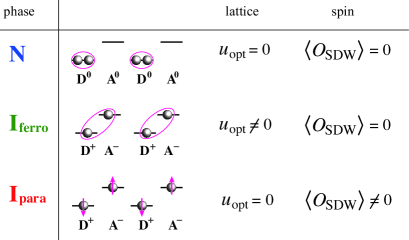
Figure 1: (Color online) Schematic view of three states observed in the NI transition systems. D and A stand for the donor and acceptor molecules, respectively, where the HOMO of the former and the LUMO of the latter are drawn. The red ellipses in the N and I_ferro states represent the singlet formation of the spins. In the I_para state, the semiclassical picture of the spin degree of freedom is the antiferromagnetic ordering, i.e., spin-density-wave (SDW). In the I_ferro state, the lattice dimerization becomes finite, while in the I_para state the SDW order parameter becomes finite in the semiclassical picture.

One of the key factors in the NI transition systems is the emergence of the multi-stable structure in the free energy, coupled to lattice deformation. This is seen in the first-order nature of the N-to-I_ferro transition; near there, characteristic domain walls between the two states are stabilized and contribute to the physical phenomena[6, 3, 9]. Moreover, related to this fact, it has been recognized that the various states can be controlled by photo-irradiations, and that TTF-CA is one of the best target materials realizing photo-induced phase transitions. [10, 11, 12, 13, 14]

Theoretical analyses of the phase competition and excitations in the NI transition systems have been performed in detail by Nagaosa and Takimoto applying Monte Carlo calculations to a microscopic model for the electron-lattice coupled system [15, 16, 17]. In particular, the fundamental excitations are interpreted as soliton formations that can be described by the phase-field description of the order parameters. [18, 19, 17] Various quantum calculations have been performed so far. [20, 21, 22, 23, 24, 25, 26, 27] Nevertheless, there are still issues to be clarified: For example, the description of the three phases seen in the experiments and their competitions from a microscopic point of view needs to be elaborated, since early works mainly focus on low-pressure states, namely, N and I_ferro. Another important aspect is the multi-stable character stressed above, which is realized numerically but has not been reproduced from the analytical phase-field approach. These are the points that we discuss in this paper.

Another motivation here is the recent experimental progress in high-pressure measurements on TTF-CA. [28, 29] As a function of pressure in the high-temperature phases, it has been observed that the resistivity exhibits a characteristic suppression[6] around the crossover region between the N and I_para states, at which the spin excitations also show an abrupt change in behaviors. A theoretical analysis of soliton excitations has been performed motivated by these findings. [30]

In this paper, we perform a comprehensive theoretical analysis of the phase competitions and excitations, on the basis of a microscopic interacting electron model taking into account the electron–phonon coupling, by paying special attention to the multi-stable properties. We follow the semiclassical analysis developed in Refs. Hara:1983vu,Fukuyama:1985jb,Tsuchiizu:2004ct, and Fukuyama:2016io. In Sect. 2, we introduce the model and apply the bosonization method to obtain the phase-variable description of the Hamiltonian. In Sect. 3, the ground-state properties of the semiclassical phase Hamiltonian are analyzed by searching the potential minima. In Sect. 4, the soliton and domain excitations are analyzed. A summary and discussions are given in Sect. 5.

2 Model Hamiltonian and Bosonization

We consider the standard one-dimensional Hubbard-type model for NI transition systems such as TTF-CA, [15, 16, 17, 31] which can describe all the three states shown in Fig. 1. The Hamiltonian is given by $H=H_{\mathrm{e}}+H_{\mathrm{e\!-\!ph}}+H_{\mathrm{ph}}$:

$$H_{\mathrm{e}}\!\!\! = \!\!\!-t\sum_{j,\sigma}\left(c_{j,\sigma}^{\dagger}c_{j+1,\sigma}+\mathrm{H.c.}\right)$$ (1a)

$${}+\Delta\sum_{j,\sigma}(-1)^{j}n_{j,\sigma}$$

$${}+U\sum_{j}n_{j,\uparrow}n_{j,,\downarrow}+V\sum_{j}n_{j}n_{j+1},$$

$$H_{\mathrm{e\!-\!ph}}\!\!\! = \!\!\!g_{P}\sum_{j,\sigma}u_{j}(-1)^{j}\left(c_{j,\sigma}^{\dagger}c_{j+1,\sigma}+\mathrm{H.c.}\right),\quad$$ (1b)

$$H_{\mathrm{ph}}\!\!\! = \!\!\!\frac{K_{\mathrm{ph}}}{2}\sum_{j}u_{j}^{2},$$ (1c)

where $c_{j,\sigma}$ is the annihilation operator of electron on the $j$-th site with spin $\sigma$, and $n_{j,\sigma}=c_{j,\sigma}^{\dagger}c_{j,\sigma}$. The site-alternating potential reflecting the alternation of the D and A molecules along the chain direction is represented by $\Delta$. We assume $\Delta>0$ without losing generality. The couplings $U$ and $V$ represent the on-site and nearest-neighbor Coulomb interactions, respectively; $H_{\mathrm{e}}$ is sometimes called the ionic (extended) Hubbard model. The quantity $u_{j}$ represents the lattice distortion; $H_{\mathrm{e\!-\!ph}}$ is the electron–phonon coupling term and the parameter $K_{\mathrm{ph}}$ is the spring constant. Here, we consider the classical phonon and focus only on the bond-alternating ($q=\pi$) distortion [31]. The average electron density is set as half-filling, taking into account the HOMO of D and the LUMO of A molecules, as shown in Fig. 1.

2.1 Bosonized Hamiltonian

Here, we represent the Hamiltonian in terms of bosonic phase-field variables[19]. By setting the lattice constant as $a$, the charge and spin density operators can be represented as [32, 26]

$$\frac{n_{j}}{a}\!\!\! \propto \!\!\!\sin(2k_{F}x+\theta)\cos\phi,$$ (2a)

$$\frac{S_{j}}{a}\!\!\! \propto \!\!\!\cos(2k_{F}x+\theta)\sin\phi,$$ (2b)

where $\theta$ ($\phi$) represents the charge (spin) phase. The Fermi momentum is $k_{F}=\pi/(2a)$.

The Hamiltonian density of the electron part is given by [26]

$$\mathcal{H}_{\mathrm{e}} = \frac{v_{\rho}}{4\pi}\left[K_{\rho}(2\pi\Pi_{\theta})^{2}+\frac{1}{K_{\rho}}(\partial_{x}\theta)^{2}\right]$$ (3a)

$${}+\frac{v_{\sigma}}{4\pi}\left[K_{\sigma}(2\pi\Pi_{\phi})^{2}+\frac{1}{K_{\sigma}}(\partial_{x}\phi)^{2}\right]$$

$${}-\frac{g_{\Delta}}{2\pi^{2}a^{2}}\sin\theta\,\cos\phi$$

$${}-\frac{g_{c}}{2\pi^{2}a^{2}}\cos 2\theta+\frac{g_{s}}{2\pi^{2}a^{2}}\cos 2\phi$$

$${}-\frac{g_{cs}}{2\pi^{2}a^{2}}\cos 2\theta\cos 2\phi,$$

where $$K_{\rho} K_{\sigma} \Pi_{\theta} \Pi_{\phi} \theta \phi g_{\Delta}=4\pi\Delta a g_{c}=(U-2V)a+O(U^{2},UV,V^{2}) g_{s}=(U-2V)a+O(U^{2},UV,V^{2}) g_{cs}=-2Va+O(U^{2},UV,V^{2})$$ and are the Tomonaga–Luttinger parameters for the charge and spin degrees of freedom. The operators and are phase fields conjugate to and , respectively. The couplings are given as , , , and . The Peierls-type electron–phonon coupling term and the lattice Hamiltonian densities read

$$\mathcal{H}_{\mathrm{e\!-\!ph}}\!\!\! = \!\!\!-\frac{ug_{\delta}}{2\pi^{2}a^{2}}\,\cos\theta\cos\phi,$$ (3b)

$$\mathcal{H}_{\mathrm{ph}}\!\!\! = \!\!\!\frac{K_{\mathrm{ph}}}{2a}u^{2},$$ (3c)

where $g_{\delta}=8\pi g_{P}a$.

As pointed out by Sandvik et al.[33], higher-order commensurability can be important in altering the character of phase transitions. The corresponding term is expressed as

$$\mathcal{H}_{\mathrm{e}}^{\prime}=-\frac{g_{2c}}{2\pi^{2}a^{2}}\,\cos 4\theta,$$ (4)

where $g_{2c}>0$. This term effectively represents the four-body interaction, which is absent in the microscopic Hubbard-type Hamiltonian; however, it can be generated through the renormalization-group (RG) procedure. The RG equation for $g_{2c}$ is given by

$$\frac{d}{dl}g_{2c}=(2-8K_{\rho})g_{2c}+cg_{c}^{2}+c^{\prime}g_{cs}^{2},$$ (5)

where $l$ is the scaling parameter of the short-distance cutoff ($a\to a\,e^{dl}$), and $c$ and $c^{\prime}$ are positive numerical constants. Since the couplings $g_{c}$ and $g_{cs}$ are generally finite, the $g_{2c}$ term can become finite with a positive sign [$g_{2c}(l)>0$] through the RG procedure $l\rightarrow\infty$. Eventually, this term can be relevant when $K_{\rho}<1/4$ and can alter the second-order phase transition into the first-order one [33]. This could be confirmed by analyzing the RG explicitly; however, we assume this term to be a priori throughout this paper, since as we will see below it drives the phase transition between N and I_ferro to the first order, consistent with results of the experiments. [7]

Semiclassical analysis is performed by neglecting the phase fields $\Pi_{\theta}$ and $\Pi_{\phi}$. Then the semiclassical Hamiltonian is

$$\mathcal{H}_{\mathrm{cl}}\!\!\! = \!\!\!\frac{v_{\rho}}{4\pi}\frac{1}{K_{\rho}}(\partial_{x}\theta)^{2}+\frac{v_{\sigma}}{4\pi}\frac{1}{K_{\sigma}}(\partial_{x}\phi)^{2}$$ (6)

$${}+\frac{1}{2\pi^{2}a^{2}}V(\theta,\phi,u).$$

The potential term is given by

$$V(\theta,\phi,u)\!\!\! = \!\!\!-g_{\Delta}\,\sin\theta\,\cos\phi$$ (7)

$${}\!\!\!-g_{c}\,\cos 2\theta+g_{s}\,\cos 2\phi-g_{2c}\,\cos 4\theta$$

$${}\!\!\!-g_{cs}\cos 2\theta\cos 2\phi$$

$${}\!\!\!-ug_{\delta}\,\cos\theta\cos\phi+\frac{\bar{K}_{\mathrm{ph}}}{2}u^{2},$$

where we have set

$$\bar{K}_{\mathrm{ph}}\equiv 2\pi^{2}a^{2}\frac{K_{\mathrm{ph}}}{a}.$$ (8)

We will investigate its ground-state properties and excitations in Sects. 3 and 4, respectively.

2.2 Order parameters

In order to characterize the N, I_ferro, and I_para states in the following, let us introduce order parameters. Following the arguments in Ref. Tsuchiizu:2004ct, we can consider the spin-density-wave (SDW), bond-charge-density-wave (BCDW), and bond-spin-density-wave (BSDW) states. They are characterized by the following order parameters:

$$\mathcal{O}_{\mathrm{SDW}}\!\!\! \equiv \!\!\!(-1)^{j}\,(n_{j,\uparrow}-n_{j,\downarrow}),$$ (9a)

$$\mathcal{O}_{\mathrm{BCDW}}\!\!\! \equiv \!\!\!(-1)^{j}(c^{\dagger}_{j,\uparrow}c_{j+1,\uparrow}+c^{\dagger}_{j,\downarrow}c_{j+1,\downarrow}+\mathrm{H.c.}),\quad\quad$$ (9b)

$$\mathcal{O}_{\mathrm{BSDW}}\!\!\! \equiv \!\!\!(-1)^{j}(c^{\dagger}_{j,\uparrow}c_{j+1,\uparrow}-c^{\dagger}_{j,\downarrow}c_{j+1,\downarrow}+\mathrm{H.c.}).\quad\quad$$ (9c)

The BCDW order parameter corresponds to the Peierls dimerization operator. By applying the bosonization, the order parameters are rewritten as [26]

$$\mathcal{O}_{\mathrm{SDW}}(x)\!\!\! \propto \!\!\!\cos\theta(x)\,\sin\phi(x),$$ (10a)

$$\mathcal{O}_{\mathrm{BCDW}}(x)\!\!\! \propto \!\!\!\cos\theta(x)\,\cos\phi(x),$$ (10b)

$$\mathcal{O}_{\mathrm{BSDW}}(x)\!\!\! \propto \!\!\!\sin\theta(x)\,\sin\phi(x).$$ (10c)

Furthermore, to characterize low-energy excitations, it is convenient to introduce topological charges $Q$ and $S_{z}$ for the charge and spin sectors, which we use to classify the soliton and domain-wall excitations. They are given by [17, 25, 26]

$$Q=\frac{1}{\pi}\int dx\,\partial_{x}\theta,\quad S_{z}=\frac{1}{2\pi}\int dx\,\partial_{x}\phi.$$ (11)

For example, in the noninteracting case with a finite $\Delta$, the lowest-energy excitation is a soliton represented by trajectory lines in the ($\theta$, $\phi$) plane, connecting two neighboring minima of the potential consisting of only one term $-g_{\Delta}\sin\theta\,\cos\phi$. Such an excitation carries the topological charge $Q=\pm 1$ and spin $S_{z}=\pm 1/2$, corresponding to a single-particle excitation in the N phase.

3 Ground-State Properties

First, we consider the ground-state properties of the semiclassical Hamiltonian Eq. (6), by assuming spatially uniform solutions. The lattice distortion can be determined by the variational approach:

$$u_{\mathrm{opt}}=\frac{g_{\delta}}{\bar{K}_{\mathrm{ph}}}\,\cos\theta\cos\phi.$$ (12)

Note that Eq. (12) takes the same form as the BCDW order parameter in Eq. (10b). By inserting Eq. (12) into Eq. (7), the potential is rewritten as

$$V(\theta,\phi,u_{\mathrm{opt}})\!\! = \!\!-g_{\Delta}\,\sin\theta\,\cos\phi$$ (13)

$${}-\tilde{g}_{c}\cos 2\theta+\tilde{g}_{s}\cos 2\phi-g_{2c}\cos 4\theta$$

$${}\!\!-\tilde{g}_{cs}\cos 2\theta\cos 2\phi,$$

where the coupling constants are renormalized as

$$\tilde{g}_{c} \equiv g_{c}+\frac{g^{2}_{\delta}}{8\bar{K}_{\mathrm{ph}}},$$ (14a)

$$\tilde{g}_{s} \equiv g_{s}-\frac{g^{2}_{\delta}}{8\bar{K}_{\mathrm{ph}}},$$ (14b)

$$\tilde{g}_{cs} \equiv g_{cs}+\frac{g^{2}_{\delta}}{8\bar{K}_{\mathrm{ph}}}.$$ (14c)

Here, we neglect the term $-g_{\delta}^{2}/(8\bar{K}_{\mathrm{ph}})$, which merely gives a constant contribution.

The resulting potential Eq. (13) is reduced to the same form to that for the purely electronic ionic extended Hubbard model without lattice distortion,[26, 33] i.e., $H_{\mathrm{e}}$ [Eq. (1a)] whose phase-field description is $\mathcal{H}_{\mathrm{e}}$ [Eq. (3a)] added by the higher-order term $\mathcal{H}_{\mathrm{e}}^{\prime}$ [Eq. (4)]. In Ref. Tsuchiizu:2004ct, $\mathcal{H}_{\mathrm{e}}$ was analyzed, including the semiclassical treatment for the ground state, which we can directly extend.

Let us make the correspondence between the phases discussed in previous works and those observed in the NI transition systems. They are characterized by the optimized lattice distortion $u_{\mathrm{opt}}$ and the SDW order parameter $\langle\mathcal{O}_{\mathrm{SDW}}\rangle$. The correspondence is summarized in Fig. 1. In the N phase, which corresponds to the BI, [25, 26] there is neither lattice dimerization nor spin ordering, i.e., $u_{\mathrm{opt}}=0$, $\langle\mathcal{O}_{\mathrm{SDW}}\rangle=0$. The I_ferro state is characterized by the finite lattice dimerization $u_{\mathrm{opt}}\neq 0$, i.e., $\langle\mathcal{O}_{\mathrm{BCDW}}\rangle\neq 0$, while the spin ordering is absent owing to the spin-singlet formation: $\langle\mathcal{O}_{\mathrm{SDW}}\rangle=0$. In the I_para phase, the spin fluctuation develops owing to the absence of the lattice distortion ($u_{\mathrm{opt}}=0$). In the semiclassical picture, such a Mott insulating state is simply described by the SDW ordering and gives $\langle\mathcal{O}_{\mathrm{SDW}}\rangle\neq 0$. If we take into account the fluctuation effects for the spin mode in terms of the RG method, the SDW ordered phase can be regarded as the paramagnetic state with predominant spin correlations. [32, 26] Namely, the positive coupling $g_{s}$ becomes marginally irrelevant and renormalized to zero $g_{s}\to 0$, indicating the absence of locking potential for the spin phase variable $\phi$: the paramagnetic gapless spin-liquid state.

When there is finite electron–phonon coupling, the one-dimensional Mott insulating state (i.e., the I_para state) is always unstable owing to the Peierls instability in the ground state ($T=0$). Thus, with decreasing temperature, the phase transition occurs from the paramagnetic I_para state into the state with static lattice dimerization (I_ferro state) where spin-singlets are formed. This is seen in the form of the effective coupling for the spin mode $\tilde{g}_{s}$ given by Eq. (14b). Once the electron–phonon coupling is introduced, the effective coupling $\tilde{g}_{s}$ turns negative at sufficiently low energy or temperature, and then the effective coupling $\tilde{g}_{s}$ flows to $-\infty$. This situation corresponds to the spin-singlet formation and then the SDW correlations decay exponentially. Therefore the I_para state is unstable at $T=0$ for finite electron–phonon coupling. However, this is not the case if we consider the states at finite temperatures, since the temperature plays a role of cutoff of the RG equation, and then the effective coupling $\tilde{g}_{s}$ can be positive. Thus the obtained I_para state in our semiclassical treatment should be regarded not as a zero-temperature phase but as a finite-temperature phase, which in fact is the case in experiments for NI transition systems.

We can find the stable points in the potential Eq. (13), by assuming spatially uniform solutions. As mentioned above, we can follow the analysis in Ref. Tsuchiizu:2004ct but here the higher-order $g_{2c}$ term $\mathcal{H}_{\mathrm{e}}^{\prime}$ [Eq. (4)] is included. The positions of the locked phase fields $\theta$ and $\phi$ are determined from the saddle-point equations $\partial V(\theta,\phi,u_{\mathrm{opt}})/\partial\theta=\partial V(\theta,\phi,u_{\mathrm{opt}})/\partial\phi=0$. The solutions of the saddle-point equations yield the following four states ($\alpha_{\theta}$ and $\alpha_{\phi}$ are nonuniversal constants), which are qualitatively the same as those in Ref. Tsuchiizu:2004ct:

• N state: The phase fields are locked at $(\theta,\phi)=(\frac{\pi}{2},0)$, $(-\frac{\pi}{2},\pi)$ (modulo $2\pi$). In this case, $u_{\mathrm{opt}}=0$ and $\langle\mathcal{O}_{\mathrm{SDW}}\rangle=0$.

• I_ferro state: The phase fields are locked at $(\theta,\phi)=(\frac{\pi}{2}\pm\alpha_{\theta},0)$ or $(-\frac{\pi}{2}\pm\alpha_{\theta},\pi)$. The lattice dimerization order parameter becomes finite ($u_{\mathrm{opt}}\propto\cos\theta\cos\phi\neq 0$) while $\langle\mathcal{O}_{\mathrm{SDW}}\rangle=0$.

• I_para state: The phase fields are locked at $(\theta,\phi)=(0,\pm\frac{\pi}{2})$ or $(\pi,\pm\frac{\pi}{2})$. The SDW order parameter becomes finite ($\langle\mathcal{O}_{\mathrm{SDW}}\rangle\propto\cos\theta\sin\phi\neq 0$), while $u_{\mathrm{opt}}=0$.

• BSDW state: The phase fields are locked at $(\theta,\phi)=(\frac{\pi}{2},0\pm\alpha_{\phi})$ or $\bigl{(}-\frac{\pi}{2},\pm(\pi-\alpha_{\phi})\bigr{)}$.

The positions of the locked phase fields $\theta$ and $\phi$ and the corresponding states are shown in Fig. 2. In the present analysis, we do not focus on the BSDW phase since this is not observed experimentally in TTF-CA. Additionally, the BSDW state cannot have a true long-range order since the phase locking of $\phi$ is prohibited, except in the spin-gapped case with $\langle\phi\rangle=0$ (mod $\pi$), owing to the spin-rotational SU(2) symmetry. [26]

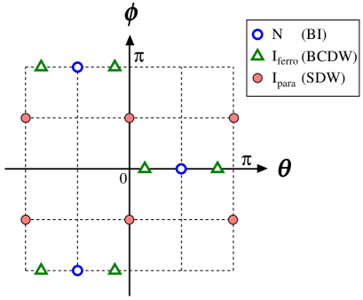
Figure 2: (Color online) Positions of the locked phase fields $\theta$ and $\phi$ in the N, I_ferro, and I_para states. The phase lockings of the N and I_ferro ground states were originally indicated in Ref.  Nagaosa:1986tb. This figure is the same as Fig. 8 in Ref. Tsuchiizu:2004ct, where N, I_ferro, and I_para correspond to the BI, BCDW, and SDW states, respectively, while the BSDW state is not shown. In Ref. Fukuyama:2016io, I_ferro is called the polarized Mott insulator.

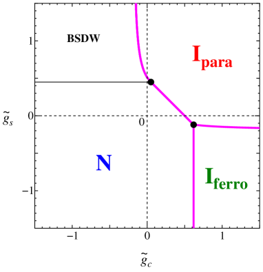
Figure 3: (Color online) Phase diagram obtained by minimizing the potential energy $V(\theta,\phi,u_{\mathrm{opt}})$ [Eq. (13)]. The parameters are chosen as $g_{\Delta}=1$, $\tilde{g}_{cs}=-0.2$, and $g_{2c}=0.1$. The thick lines indicate the first-order phase transitions, while the thin line indicates the second-order phase transition. In the case of $g_{2c}=0$, the phase boundary between N and I_ferro becomes of the second order.[26] The numerically-obtained triple point between the I_para, I_ferro, and N states is $(\tilde{g}_{c},\tilde{g}_{s})\approx(0.619,-0.119)$. The triple point of the I_para, N, and BSDW states is $(\tilde{g}_{c},\tilde{g}_{s})=(0.05,\,0.45)$. The lattice dimerization occurs ($u_{\mathrm{opt}}\neq 0$) in the I_ferro and BSDW states.

The analysis without the higher-order term ($g_{2c}=0$) yields the phase diagram in Fig. 10 of Ref. Tsuchiizu:2004ct, where the “BI”, “BCDW”, and “SDW” phases correspond to the N, I_ferro, and I_para states, respectively. Owing to the presence of the $\tilde{g}_{cs}$ term that couples the charge and spin phase variables, the direct transition between N and I_para occurs in a finite parameter range and its phase transition is of the first order. However, the transition between N and I_ferro was found to always be of the second order, and then the experimental observations in TTF-CA could not be reproduced. The introduction of the $g_{2c}$ term changes it to a first-order transition. Once the $g_{2c}$ term is introduced, although analytical evaluations of the phase boundaries are complicated, here we obtain the phase diagram for a finite value of $g_{2c}$ by numerically finding the potential minima of $V(\theta,\phi,u_{\mathrm{opt}})$, as shown in Fig. 3. We find that the phase boundary between the N and I_ferro states becomes of the first order in contrast to the previous analysis, owing to the presence of the higher-order commensurability term $\sim\cos 4\theta$. In other words, near the first-order phase boundary, a multi-stable character between the N and I states is seen, then the NI domain walls can be discussed as in the next section.

Incidentally, the phase boundary between the I_para and I_ferro states also becomes of the first order. This first-order behavior is seen even for $g_{2c}=0$ and can be ascribed to the spin-charge coupling $g_{cs}$ term. [26] As already clarified in Ref. Tsuchiizu:2004ct, this first-order behavior is an artifact due to the semiclassical treatment and changes into the second-order transition if we take into account the fluctuation effect in terms of the RG method. This is consistent with the spin-Peierls transition in the $S=1/2$ Heisenberg chain coupled with lattice distortions, where the gapless spin liquid turns into a spin-gapped dimerized state. It shows a second-order phase transition in general[34]. It is also consistent with the experiments where the I_para–I_ferro transition as a function of temperature is continuous, [7, 35] in contrast with the first-order nature of the N–I_ferro transition.

4 Soliton and Domain Formations

In this section, we examine the excited states, namely, the soliton and domain formations. By taking into account the spatial variations of the phase fields $\theta$ and $\phi$ and also of the lattice distortion $u$, our semiclassical Hamiltonian density [Eq. (6)] is given by

$$\mathcal{H}_{\mathrm{cl}}\!\! = \!\!\frac{v_{\rho}}{4\pi}\frac{1}{K_{\rho}}[\partial_{x}\theta(x)]^{2}+\frac{v_{\sigma}}{4\pi}\frac{1}{K_{\sigma}}[\partial_{x}\phi(x)]^{2}$$ (15)

$${}+\frac{1}{2\pi^{2}a^{2}}V\bigl{(}\theta(x),\phi(x),u(x)\bigr{)},$$

where the spatial variation of the lattice distortion is now explicitly shown [$u\to u(x)$]. The lattice distortion $u(x)$ can again be determined from the variational approach:

$$u_{\mathrm{opt}}(x)=\frac{g_{\delta}}{\bar{K}_{\mathrm{ph}}}\cos\theta(x)\cos\phi(x).$$ (16)

In the semiclassical approach, possible soliton/domain excitations from the ground state are described as variational solutions of the following simultaneous equations

$$0\!\!\! = \!\!\!\frac{\pi v_{\rho}a^{2}}{K_{\rho}}\frac{\partial^{2}\theta(x)}{\partial x^{2}}+g_{\Delta}\cos\theta(x)\cos\phi(x)$$ (17a)

$${}-2\tilde{g}_{c}\sin 2\theta(x)-4g_{2c}\sin 4\theta(x)$$

$${}-2\tilde{g}_{cs}\sin 2\theta(x)\cos 2\phi(x),$$

$$0\!\!\! = \!\!\!\frac{\pi v_{\sigma}a^{2}}{K_{\sigma}}\frac{\partial^{2}\phi}{\partial x^{2}}-g_{\Delta}\sin\theta(x)\sin\phi(x)$$ (17b)

$${}+2\tilde{g}_{s}\,\sin 2\phi$$

$${}-2\tilde{g}_{cs}\cos 2\theta(x)\sin 2\phi(x).$$

The characters of all the possible excitations discussed in the following are summarized in Table 1. In the following, we show results for the fixed condition $g_{\Delta}=1$, $\tilde{g}_{cs}=-0.2$, $g_{2c}=0.1$, $v_{\rho}=v_{\sigma}=2$, $K_{\rho}=0.3$, and $K_{\sigma}=1$.

4.1 Soliton excitations

By solving Eq. (17) numerically, [36] we can analyze possible excitations. We obtain various types of excitations depending on the choice of the parameters. The typical soliton excitations in the three phases are shown in Fig. 4, showing the spatial variations of the phase fields [(a), (d), (g)] and the order parameters [(b), (e), (h)] as well as the trajectories in the ($\theta$, $\phi$) plane [(c), (f), (i)].

The soliton excitations in the N and I_ferro states are consistent with those discussed in Ref. Nagaosa:1986tb. Namely, in the N state, a possible soliton is the so-called polaron excitation. The polaron is described by the local lattice distortion and carries $|Q|=1$ and $|S_{z}|=1/2$, adiabatically connected to the single-particle excitation in the non-interacting case mentioned in Sect. 2.2. In the I_ferro state, two excitations are possible. One is the charge soliton, and the other is the spin soliton. In both excitations, the topological charge $Q$ of the lowest-energy excitation becomes fractional, reflecting the nonuniversal values of the minima of the potential.

In the I_para state, the soliton excitation connecting potential minima along the $\theta$ direction is the charge soliton. Note that the charge soliton profile on the $\theta$–$\phi$ plane largely deviates from a straight line. Owing to this fact, as seen in Fig. 4(h), it is accompanied by the local lattice distortion. In this sense, this charge soliton is different from the charge excitation in the prototypical one-dimensional Mott insulator. We can also consider the spin soliton, which connects the potential minima along the $\phi$ direction. The spin soliton is accompanied by the local lattice distortion as well. However, note that this behavior is in contrast to the charge soliton: In the case of the charge soliton, the lattice distortion disappears if the soliton profile is the straight line on the $\theta$–$\phi$ plane (i.e., $\langle\phi\rangle=\pi/2$ mod $\pi$), while the spin soliton always carries the lattice distortion even if the spin soliton profile is described by the straight line (i.e., $\langle\theta\rangle=0$ mod $\pi$). This is because of the presence of the term $\cos\theta(x)\cos\phi(x)$ in Eq. (16). We find $\cos\langle\phi\rangle=0$ in the case of a straight-line charge soliton, while $\cos\langle\theta\rangle=\pm 1$ in the case of a straight-line spin soliton. Furthermore, we also observe a charge-spin coupled excitation, connecting the minima, e.g., $(\theta,\phi)=(0,\pi/2)$ and $(\pi,-\pi/2)$: This carries $|Q|=1$ and $|S_{z}|=1/2$. Its profile shown in the dashed line in Fig. 4(i) is different from the isolated charge or spin solitons and then we call this “charge+spin” soliton. When we decrease $\tilde{g}_{c}$, the profile of this charge+spin soliton smoothly connects to that of the charge soliton.

Table 1: Characters of excitations: charge soliton (CS), spin soliton (SS), charge$+$spin soliton (CSS), and domain wall (DW). The “phase change” indicates that the pattern of the lattice distortion changes across the excitation position, e.g., $u_{\mathrm{opt}}(x)>0(<0)$ for $x>x_{e}$ ($x<x_{e}$), where $x_{e}$ is the location of the excitation. The “local distortion^∗” indicates the asymmetric local lattice distortion, i.e., $u_{\mathrm{opt}}(x_{e}+\delta x)=-u_{\mathrm{opt}}(x_{e}-\delta x)$.

Excitation	Charge $|Q|$	Spin $|S_{z}|$	Lattice distortion	Ref.
Polaron in N	1	$1/2$	Local distortion∗	Nagaosa:1986tb
CS in Iferro	$2\alpha_{\theta}/\pi$	0	Phase change	Nagaosa:1986tb,Fukuyama:1985jb
SS in Iferro	$1-2\alpha_{\theta}/\pi$	$1/2$	Phase change	Nagaosa:1986tb,Fukuyama:1985jb
CS in Ipara	1	0	Local distortion∗
SS in Ipara	0	$1/2$	Local distortion
CSS in Ipara	1	$1/2$	Local distortion∗
N–Iferro DW	$\alpha_{\theta}/\pi$	0	Zero$\leftrightarrow$Finite
N–Ipara DW	$1/2$	$1/4$	Local distortion
Iferro–Ipara DW	$1/2-\alpha_{\theta}/\pi$	$1/4$	Finite$\leftrightarrow$Zero

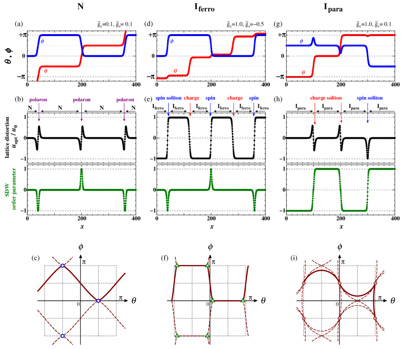
Figure 4: (Color online) Soliton excitations in different phases: N (a-c), I_ferro (d-f), and I_para (g-i). The parameters are chosen as $(\tilde{g}_{c},\tilde{g}_{s})=(0.1,\,0.1)$ for the N state, $(1.0,\,-0.5)$ for the I_ferro state, and $(1.0,\,0.1)$ for the I_para state. The spatial variations of the phase fields $\theta$ and $\phi$ are shown in (a), (d), and (g). The variations of the order parameters $u_{\mathrm{opt}}$ and $\langle\mathcal{O}_{\mathrm{SDW}}\rangle$ are shown in (b), (e), and (h). The corresponding trajectories on the plane of $\theta$ and $\phi$ are shown by the solid lines in (c), (f), (i), where the other possible trajectories are indicated by the dashed lines.

4.2 Soliton formation energies

From the results above, we evaluate the soliton formation energies across the NI phase boundaries, keeping in mind the experimental system showing the phase transition/crossover by changing temperature and pressure. In particular, we pay attention to the possible excitations contributing to the electric conductivity.

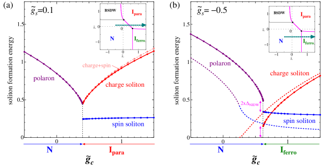
Figure 5: (Color online) Soliton formation energies across the boundary between N and I_para (a) and the boundary between N and I_ferro (b). In (b), the case for $g_{\delta}=g_{s}=g_{cs}=g_{2c}=0$ [30] is shown by the dashed lines. The difference between the excitation energies of a polaron and a spin soliton ($\Delta_{\mathrm{polaron}}-\Delta_{\mathrm{spin}}$) at the phase boundary ($\tilde{g}_{c}\approx 0.62$), as well as the charge-soliton excitation energy, corresponds to twice the excitation gap of the NIDW (see text). In the insets, the adopted parameters in Fig. 3 are shown.

The results for soliton excitations across the boundary between the N and I_para states are shown in Fig. 5(a). For small $\tilde{g}_{c}$, the system is in the N phase and the fundamental excitation is given by the polaron. For large $\tilde{g}_{c}$, the system is in the I_para state and the possible excitations are charge, spin, and charge+spin solitons. We observe that the excitation energy of charge+spin soliton is always slightly larger than that of the charge soliton. In the I_para state, the spin soliton does not carry a charge and thus does not contribute to electric conductivity. Thus electric conduction is possible through excitations of the polaron soliton and the charge and charge+spin solitons in the N and I_para phases, respectively. As seen in Fig. 5(a), all of their excitation energies become sufficiently suppressed, monotonically toward the phase boundary. On the phase boundary ($\tilde{g}_{c}=0.4$), the excitation energy of the polaron and that of the charge soliton coincide.

The soliton excitation energies across the boundary between the N and I_ferro states are shown in Fig. 5(b). In the I_ferro state, both the charge and spin solitons are responsible for the electric conductivity, [17, 30] since both carry the topological (fractional) charge $Q$. With increasing $\tilde{g}_{c}$, in the N phase, the polaron excitation energy decreases. On the other hand, in the I_ferro phase, the charge-soliton excitation energy increases, while that of the spin soliton decreases. Such a behavior is seen as well in the case of $g_{\delta}=g_{s}=g_{cs}=g_{2c}=0$, which corresponds to the results of Ref. Fukuyama:2016io. This is seen in the dashed lines in Fig. 5(b): the polaron excitation energy smoothly connects to the spin-soliton excitation energy across the phase boundary. In the present case with $g_{2c}\neq 0$, there is a gap between them owing to the first-order nature of the phase transition.

In both cases above, just at the phase boundaries, there are relations between the soliton formation energies of the two phases when approaching from both sides of the critical values. There, domain-wall excitations become possible as discussed in previous works, which we discuss in the next subsection.

4.3 Domain walls

In this subsection, we analyze the possible excitations at the phase boundaries. At the phase boundaries, domain excitations become possible in addition to the soliton excitations. In previous theoretical and experimental works, [16, 3, 10, 11, 9, 13, 4, 24, 37, 5, 28, 29] the domain wall between the N and I states (abbreviated as NIDW) has been discussed as a possible fundamental excitation near the NI phase transition point. However, the explicit descriptions of the NIDW were not given in terms of the phase-field ($\theta,\phi$) description as mentioned in Sect. 1, since the multi-stable character of the N and I_ferro states could not be realized. In the present analysis, in contrast, the multi-stable structure of the potential is realized by taking into account the higher-order commensurability potential and thus it is now possible to give explicit descriptions of NIDW.

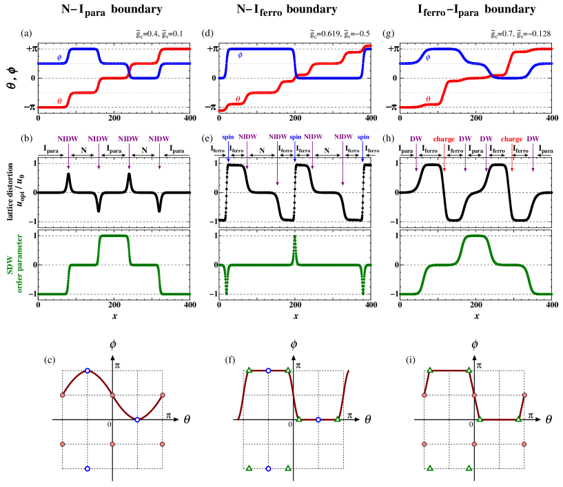
Figure 6: (Color online) Domain and soliton excitations at the N–I_para boundary (a-c), at the N–I_ferro boundary (d-f), and at the I_ferro–I_para boundary (g-i), where the parameters are chosen as $(\tilde{g}_{c},\tilde{g}_{s})=(0.4,\,0.1)$, $(0.619,\,-0.5)$, and $(0.7,\,0.128)$, respectively. The notations are the same as in Fig. 4.

Figure 6 shows lowest-energy excitations on the various phase boundaries with the boundary conditions $Q=2$ and $S_{z}=0$. Owing to the finite value of $Q$, they can carry electronic currents when an electric field is applied. In the following, possible excitations are analyzed in the respective cases.

4.3.1 N–I${}_{\mbox{\scriptsize{para}}}$ boundary

At the phase boundary between the N and I_para states, the only stable excitation is the NIDW [Figs. 6(a)$-$6(c)]. In this case, the potential $V(\theta,\phi,u_{\mathrm{opt}})$ takes minima at, e.g., $(\theta,\phi)=(\pi/2,0)$ (corresponding to the N state) and $(\theta,\phi)=(0,\pi/2)$ (corresponding to the I_para state). The NIDW is described by the excitation connecting these minima. In order to distinguish this from the NIDW discussed in the next subsection, we call this “N–I_para DW”. As we will see below, this N–I_para DW smoothly connects to the polaron in the N phase [Fig. 4(c)] or to the charge soliton in the I_para phase [Fig. 4(i)] if we move away from the phase boundary. This is the reason why the polaron excitation energy and the charge-soliton excitation energy coincide at the boundary [Fig. 5(a)]. Here it is worth noting that the lattice distortion occurs locally at the N–I_para DW. This is natural since the polaron in the N phase and the charge soliton in the I_para phase both have such a character.

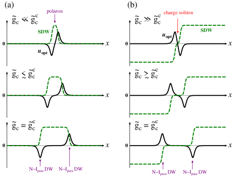
Figure 7: (Color online) Generations of the N–I_para DWs when approaching the N–I_para boundary from the N state (a) and from the I_para state (b), where we fixed $\tilde{g}_{s}=0.1$. The solid lines denote the spatial variations of $u_{\mathrm{opt}}$ and the dashed lines denote those of the SDW order parameter $\langle\mathcal{O}_{\mathrm{SDW}}\rangle$. The polaron in the N state (a) splits into a pair of the N–I_para DWs, and the region sandwiched by them is the I_para state where $\langle\mathcal{O}_{\mathrm{SDW}}\rangle\neq 0$. The charge soliton in the I_para state (b) splits into a pair of the N–I_para DWs and the sandwiched region is the N state where $u_{\mathrm{opt}}=\langle\mathcal{O}_{\mathrm{SDW}}\rangle=0$.

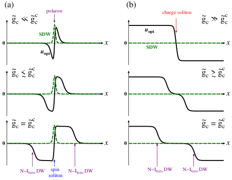
Figure 8: (Color online) Generations of the N–I_ferro DWs when approaching the N–I_ferro boundary from the N state (a) and from the I_ferro state (b), where we fixed $\tilde{g}_{s}=-0.5$. The notations are the same as those in Fig. 7. The polaron in the N state (a) splits into two N–I_ferro DWs and a single spin soliton, where the lattice-distorted region of the polaron is expanded and changes into the I_ferro state. The charge soliton in the I_ferro state (b) splits into a pair of the N–I_ferro DWs and the lattice-relaxed region is the N state.

The polaron in the N phase can be considered as a confined particle of the pair of the local lattice distortion $u>0$ and $u<0$. The N–I_para DW can be regarded as a dissociation of this pair of lattice distortion, i.e., the single polaron is deconfined into two N–I_para DWs at the phase boundary and the I_para state emerges as an intervening state between them, as shown in Fig. 7(a). This picture is in accord with the observation that the single polaron carries the charge $|Q|=1$ and the spin $|S_{z}|=1/2$, while the single N–I_para DW carries $|Q|=1/2$ and $|S_{z}|=1/4$. Similarly, approaching from the I_para phase, the charge soliton is dissociated to a pair of N–I_para DW, as shown in Fig. 7(b). This picture is also in accord with the conservation of the topological charge and spin.

4.3.2 N–I${}_{\mbox{\scriptsize{ferro}}}$ boundary

At the phase boundary between the N and I_ferro states, two kinds of excitations are possible [Figs. 6(d)$-$6(f)]. One is the NIDW, sometimes called [17] the lattice relaxed (LR-) NIDW, and the other is the spin soliton. In this case, the potential takes minima at, e.g., $(\theta,\phi)=(\pi/2,0)$ and $(-\pi/2,\pi)$ (corresponding to the N state) and $(\theta,\phi)=(\pi/2\pm\alpha_{\theta},0)$ and $(-\pi/2\pm\alpha_{\theta},\pi)$ (corresponding to the I_ferro state). The NIDW is described by the excitation connecting the minima, e.g., $(\theta,\phi)=(\pi/2,0)$ and $(\pi/2-\alpha_{\theta},0)$. This can be called “N–I_ferro DW”. On the other hand, the spin soliton is described by the excitation connecting the minima, e.g., $(\theta,\phi)=(\pi/2-\alpha_{\theta},0)$ and $(-\pi/2+\alpha_{\theta},\pi)$, where we assumed $\alpha_{\theta}>0$.

When we approach the phase boundary from the N state, we can observe that the single polaron (connecting $(-\pi/2,\pi)$ and $(\pi/2,0)$) splits into two N–I_ferro DWs and the single spin soliton [see Fig. 8(a)]. Then at the N–I_ferro boundary, we can obtain the relation

$$\Delta_{\mathrm{polaron}}=2\Delta_{\mathrm{N\!-\!I_{ferro}DW}}+\Delta_{\mathrm{spin}},$$ (18)

where $\Delta_{\mathrm{polaron}}$, $\Delta_{\mathrm{N\!-\!I_{ferro}DW}}$, and $\Delta_{\mathrm{spin}}$ are the respective formation energies. Therefore the gap in energy of the polaron and spin excitations observed in Fig. 5(b) can be understood as $2\times\Delta_{\mathrm{N\!-\!I_{ferro}DW}}$.

On the other hand, when we approach the phase boundary from the I_ferro state, the single charge soliton splits into two N–I_ferro DWs [see Fig. 8(b)]. Thus we obtain

$$\Delta_{\mathrm{charge}}=2\Delta_{\mathrm{N\!-\!I_{ferro}DW}},$$ (19)

where $\Delta_{\mathrm{charge}}$ is the formation energy of the charge soliton. These pictures are in accord with the neutrality of the topological charge $Q$ and spin $S_{z}$. From Fig. 6(f), we can see that the single N–I_ferro DW carries $|Q|=\alpha_{\theta}/\pi$ and $|S_{z}|=0$, while the charge soliton in the I_ferro state carries $|Q|=2\alpha_{\theta}/\pi$ and $|S_{z}|=0$, and the spin soliton carries $|Q|=1-2\alpha_{\theta}/\pi$ and $|S_{z}|=1/2$.

4.3.3 I${}_{\mbox{\scriptsize{ferro}}}$–I${}_{\mbox{\scriptsize{para}}}$ boundary

At the boundary between the I_ferro and I_para states [Figs. 6(g)$-$6(i)], the two kinds of excitations are possible. One is the DW between I_ferro and I_para (I_ferro–I_para DW). The other excitation is the charge soliton. As seen from Fig. 6(i), the I_ferro–I_para DW carries the topological charge $Q=1/2-\alpha_{\theta}/\pi$ and spin $S_{z}=1/4$.

We note that, as mentioned in Sect. 3, the first-order phase boundary between I_ferro and I_para should be replaced with a second-order one if we take into account the fluctuation effect. Therefore the DW here, stabilized owing to the multi-stable structure of the potential, is not stabilized. Nevertheless, if a first-order phase transition is realized beyond our model, the DW structure here will be relevant.

5 Summary and Discussion

In summary, we have performed comprehensive analyses of the competing states in the neutral–ionic transition systems, from the semiclassical treatment of the bosonized Hamiltonian. By taking into account the higher-order commensurability potentials, the transition between the N state and the I_ferro state is transformed from a second-order phase transition to a first-order phase transition, in accordance with the experiments. Soliton excitations have been examined explicitly and the soliton formation energies have been evaluated. At the phase boundaries, we have given the explicit description of different types of domain-wall excitations, and investigate their relations with the soliton excitations in the respective phases. The characters of the soliton and domain-wall excitations have been classified in terms of the topological charge and spin.

Let us discuss the relevance of our results to the experimentally-observed phase diagram in TTF-CA.[7] The renewed phase diagram of TTF-CA has been determined recently on the plane of temperature and pressure, where the phase competitions among N, I_ferro, and I_para were observed.[29] The competitions of these states can be reproduced in Fig. 3, given that the I_para state is described by the SDW ordered state in our semiclassical theory. As mentioned in Sect. 3, it is known from previous theoretical works that this SDW ordering becomes quasi-long ranged if we take the 1D quantum fluctuation effects into account, thus the paramagnetic Mott insulating state can be observed instead. This paramagnetic Mott insulating state is a finite temperature phase which is unstable toward the spin-Peierls dimerization, i.e., the I_ferro state, as was discussed in Sect. 3 as well. The first-order N–I_para phase boundary is expected to turn into a crossover at high temperatures, since there is no symmetry breaking now because the corresponding Mott insulating state has no spin ordering. From these correspondences, our results are consistent with the experimental phase diagram, as well as with recent numerical results. [27]

Next, we discuss the characteristic behavior of resistivity, where a sharp minimum as a function of pressure was observed in the high-temperature crossover region between the N and I_para states. [6, 28, 29] In the low-pressure N state, the lowest-energy excitation is the polaron that carries a charge. Therefore, the rapid decrease in soliton formation energy seen in Fig. 5 toward the phase boundary is consistent with the decrease in the resistivity in experiments. On the other hand, as for the I_ferro state, it was claimed in Ref. Nagaosa:1986tb that the activation energy in conductivity is determined by the larger excitation energy of the spin or charge soliton, i.e., by the rate-determining step. In Ref. Fukuyama:2016io, in contrast, the activation energy was considered to be determined by the sum of excitation energies of charge and spin solitons. If we apply these interpretations to the present results across the N–I_ferro boundary [Fig. 5(b)], both interpretations indicate that the resistivity takes a minimum away from the N–I_ferro boundary. Instead, the soliton formation energies across the N–I_para boundary [Fig. 5(a)] suggest the resistivity minimum to coincide with the transition point between the N and I_para states. This is because, in the I_para state, the low-energy excitations carrying electric current are the charge and charge+spin solitons, both showing a monotonic and steep increase in formation energies by going away from the phase boundary. The distinction of the two scenarios is possible by experimentally determining the pressure where the phase transformation takes place and comparing with the pressure for the resistivity minimum. The former can be extracted, e.g., by analyzing the pressure dependence of the charge transfer $\rho$, although it is a crossover, which seems to support the latter interpretation. [29]

Here we briefly discuss the magnitude of the excitation gap at the boundary between the N and I_para states. In TTF-CA, the minimum activation energy was evaluated as $E\approx 0.055$ eV. [29] To make a qualitative comparison between this activation energy and the present results, we should take into account the quantum fluctuations in the electron parts of the Hamiltonian and go beyond the adiabatic treatment of the lattice distortion. In addition, the excitation gap at the boundary sensitively depends on the magnitude of the dynamically-generated $g_{2c}$ term in Eq. (5), whose qualitative estimation is difficult. Here let us just argue about possible roles of the quantum fluctuations due to the $\Pi_{\theta}$ and $\Pi_{\phi}$ terms in Eq. (3a), and the effect of phonon dynamics. The present semiclassical treatment of the electron part can be justified when $K_{\nu}\ll 1$ ($\nu=\rho,\sigma$). It is known that the soliton formation energy is reduced when quantum fluctuations are included: For example, the soliton formation gap induced only by the $g_{c}\cos 2\theta$ term (simple quantum sine-Gordon model), which is given by $\sim\sqrt{g_{c}}$ in the classical limit, is given by $\sim g_{c}^{1/(2-2K_{\rho})}$ for a general value of $K_{\rho}(<1)$. [38, 39] As for the spin part, the excitation gap in the I_para vanishes if we take the 1D quantum fluctuation effects into account, as discussed before. Regarding the dynamical phonon, we can expect that the excitation gap will sufficiently be reduced if the gap is smaller than the Debye frequency, as has been indicated in the context of the spin-Peierls chain. [40] All these effects can be taken into account by using the RG method, [41, 42] whose application to the full Hamiltonian in this case for the quantitative evaluation of the soliton excitation gap is left for future works.

We note that the character of spin excitations at the N–I_ferro boundary is completely different from that at the N–I_para boundary. In the former, the elementary spin excitation is a spin soliton, which essentially should show an activation behavior in the spin susceptibility in the dilute limit. In the latter, it will be paramagnetic excitations as seen in the Heisenberg spin chain; therefore every D and A site carries effective $S=1/2$ interacting along the chain. Nevertheless, we note that the temperature dependence of spin susceptibility can largely deviate from the Bonner–Fisher behavior, owing to the renormalization effects by the terms absent in the simple Hubbard model but present here, e.g., the site-alternating potential term and the electron–phonon coupling. In fact, in tetrathiafulvalene-$p$-bromanil (TTF-BA), [35] the spin susceptibility in the I_para phase shows paramagnetic behavior above the transition temperature to the I_ferro ground state, but does not follow the Bonner–Fisher behavior. In addition, as shown in Sect. 4.1, we found that the spin soliton in the I_para state is accompanied by local lattice distortion. In this sense, our spin soliton excitation is different from the conventional spinon excitations, and can be regarded as a “spin-polaron” excitation. The local/dynamic lattice distortions have actually been observed in the high-temperature crossover region in TTF-CA under pressure in the optical measurements, [9] whose relevance to such a novel excitation might be an interesting future problem.

Finally, let us comment on experimental observations of photo-induced phenomena in NI systems, especially in the I_ferro phase of TTF-CA, which is prominent among many. In Ref. Iwai:2002ip, an I_ferro-to-N conversion into stable macroscopic N domains induced by pulse optical excitations is reported. A notable point is that, when the temperature is just below the transition temperature $T_{\mathrm{NI}}$, the conversion occurs irrespective of the excitation density by light, whereas at low temperature, a high density is needed. This is consistent with the multi-stable structure of free energy discussed in this paper and with the stability of N–I_ferro DW just at the transition point. In our calculations, when the system is deeply in the I_ferro phase, DW excitations are not stable; they will pair annihilate into a polaron excitation [the inverse process of Fig. 8(a)], and therefore multiplication of the excited N state is hampered. However, since the present calculations are based on classical phonons, its direct application to one-dimensional “string” excitations implicated in experiments is not straightforward, but may rather serve to describe the macroscopic domain of the N state in the I_ferro background observed at a later time scale of the order of $100$ ps; the oscillation of such a domain is suggested in Ref. Iwai:2002ip.

References

- [1] H. M. McConnell, B. M. Hoffman, and R. M. Metzger, Proc. Natl. Acad. Sci. USA 53, 46 (1965).
- [2] J. B. Torrance, J. E. Vazquez, J. J. Mayerle, and V. Y. Lee, Phys. Rev. Lett. 46, 253 (1981).
- [3] H. Okamoto, T. Mitani, Y. Tokura, S. Koshihara, T. Komatsu, Y. Iwasa, T. Koda, and G. Saito, Phys. Rev. B 43, 8224 (1991).
- [4] S. Horiuchi, T. Hasegawa, and Y. Tokura, J. Phys. Soc. Jpn. 75, 051016 (2006).
- [5] S. Tomić and M. Dressel, Rep. Prog. Phys. 78, 096501 (2015).
- [6] T. Mitani, Y. Kaneko, S. Tanuma, Y. Tokura, T. Koda, and G. Saito, Phys. Rev. B 35, 427 (1987).
- [7] M. H. Lemée-Cailleau, M. Le Cointe, H. Cailleau, T. Luty, F. Moussa, J. Roos, D. Brinkmann, B. Toudic, C. Ayache, and N. Karl, Phys. Rev. Lett. 79, 1690 (1997).
- [8] A. Dengl, R. Beyer, T. Peterseim, T. Ivek, G. Untereiner, and M. Dressel, J. Chem. Phys. 140, 244511 (2014).
- [9] H. Matsuzaki, H. Takamatsu, H. Kishida, and H. Okamoto, J. Phys. Soc. Jpn. 74, 2925 (2005).
- [10] S. Iwai, S. Tanaka, K. Fujinuma, H. Kishida, H. Okamoto, and Y. Tokura, Phys. Rev. Lett. 88, 057402 (2002).
- [11] H. Okamoto, Y. Ishige, S. Tanaka, H. Kishida, S. Iwai, and Y. Tokura, Phys. Rev. B 70, 165202 (2004).
- [12] Y. Tokura, J. Phys. Soc. Jpn. 75, 011001 (2006).
- [13] S. Iwai, Y. Ishige, S. Tanaka, Y. Okimoto, Y. Tokura, and H. Okamoto, Phys. Rev. Lett. 96, 057403 (2006).
- [14] H. Uemura and H. Okamoto, Phys. Rev. Lett. 105, 258302 (2010).
- [15] N. Nagaosa and J. Takimoto, J. Phys. Soc. Jpn. 55, 2735 (1986).
- [16] N. Nagaosa and J. Takimoto, J. Phys. Soc. Jpn. 55, 2745 (1986).
- [17] N. Nagaosa, J. Phys. Soc. Jpn. 55, 2754 (1986).
- [18] J. Hara and H. Fukuyama, J. Phys. Soc. Jpn. 52, 2128 (1983).
- [19] H. Fukuyama and H. Takayama, in Electronic Properties of Inorganic Quasi-One-Dimensional Compounds, I (Springer Netherlands, Dordrecht, 1985) p. 41.
- [20] T. Egami, S. Ishihara, and M. Tachiki, Science 261, 1307 (1993).
- [21] S. Ishihara, T. Egami, and M. Tachiki, Phys. Rev. B 49, 8944 (1994).
- [22] K. Yonemitsu, Phys. Rev. B 65, 085105 (2002).
- [23] J. Kishine, T. Luty, and K. Yonemitsu, Phys. Rev. B 69, 075115 (2004).
- [24] Z. G. Soos and A. Painelli, Phys. Rev. B 75, 155119 (2007).
- [25] M. Fabrizio, A. Gogolin, and A. A. Nersesyan, Phys. Rev. Lett. 83, 2014 (1999).
- [26] M. Tsuchiizu and A. Furusaki, Phys. Rev. B 69, 035103 (2004).
- [27] Y. Otsuka, H. Seo, K. Yoshimi, and T. Kato, Physica B 407, 1793 (2012).
- [28] R. Takehara, K. Miyagawa, K. Kanoda, T. Miyamoto, H. Matsuzaki, H. Okamoto, H. Taniguchi, K. Matsubayashi, and Y. Uwatoko, Physica B 460, 83 (2015).
- [29] R. Takehara, Dr. Thesis, University of Tokyo (2014).
- [30] H. Fukuyama and M. Ogata, J. Phys. Soc. Jpn. 85, 023702 (2016).
- [31] M. J. Rice and E. J. Mele, Phys. Rev. Lett. 49, 1455 (1982).
- [32] M. Tsuchiizu and A. Furusaki, Phys. Rev. Lett. 88, 056402 (2002).
- [33] A. Sandvik, L. Balents, and D. K. Campbell, Phys. Rev. Lett. 92, 236401 (2004).
- [34] T. Nakano and H. Fukuyama, J. Phys. Soc. Jpn. 50, 2489 (1981).
- [35] F. Kagawa, S. Horiuchi, M. Tokunaga, J. Fujioka, and Y. Tokura, Nat. Phys. 6, 169 (2010).
- [36] M. Tsuchiizu and Y. Suzumura, Phys. Rev. B 77, 195128 (2008).
- [37] M. Masino, A. Girlando, and A. Brillante, Phys. Rev. B 76, 064114 (2007).
- [38] A. O. Gogolin, A. A. Nersesyan, and A. M. Tsvelik, Bosonization and Strongly Correlated Systems (Cambridge University Press, Cambridge, 1998).
- [39] Al. B. Zamolodchikov, Int. J. Mod. Phys. A 10, 1125 (1995).
- [40] R. Citro, E. Orignac, and T. Giamarchi, Phys. Rev. B 72, 024434 (2005).
- [41] L. G. Caron and C. Bourbonnais, Phys. Rev. B 29, 4230 (1984).
- [42] T. Giamarchi, Quantum Physics in One Dimension (Oxford University Press, Oxford, 2003).