Integrable order parameter dynamics of globally coupled oscillators

Abstract

We study the nonlinear dynamics of globally coupled nonidentical oscillators in the framework of two order parameter (mean field and amplitude-frequency correlator) reduction. The main result of the paper is the exact solution of a corresponding nonlinear system on a two-dimensional invariant manifold. We present a complete classification of phase portraits and bifurcations, obtain explicit expressions for invariant manifolds (a limit cycle among them) and derive analytical solutions for arbitrary initial data and different regimes.

1 Introduction

Frequency synchronization of nonlinear interacting oscillators is one of the most common phenomena in nature. The phenomenon discovered by Huygens in the 17th century was found out later in astronomy, chemistry and electronics, and manifests itself in various technical devices, environmental systems and nuclear physics. Today, the direction of research has shifted to studying complex nonlinear dynamical systems with global interaction such as the cooperative dynamics of laser arrays and arrays of Josephson junctions; different forms of collective behavior of insects, birds, animals and human communities; adjustment of heart rate and respiration, synchronization of electrical potentials of brain neurons and so on. Recently new phenomena such as, for example, the partial synchronization, clustering and chimera states have been revealed. There is a large and rapidly increasing amount of literature on the collective oscillatory behavior among which one can find already classic books by Kuramoto [1], Strogatz [2, 3], and Pikovsky et al. [4], the review by Asebron et al [5], and the recent brief but very informative review by Pikovsky and Rosemblum [6] on the progress and perspectives of studies of globally coupled oscillators.

Despite the apparent diversity of the phenomena emerging in ensembles of interacting nonlinear oscillators, many of them can be modeled by a system of equations based on the Stuart-Landau one, which is closely associated with the phenomenon of the supercritical Hopf bifurcation. Y. Kuramoto was the first to describe synchronization transition in oscillatory reaction-diffusion systems [7, 1] reducing the system of globally coupled Stuart-Landau equations to the system of the coupled phase oscillators known now as the famous Kuramoto model. Later the amplitude-phase dynamics was reinstated in a series of papers [8, 9, 10, 11]. The mixed amplitude-phase dynamics significantly expanded a range of phenomena elucidated with the Kuramoto model. Depending on the ratio between the amount of interaction and the deviation of natural oscillator frequencies, new regimes of collective behavior such as amplitude death, quenched amplitude, oscillations with large amplitude, collective chaos and intermediate mixed states can arise.

The system of equations describing the dynamics of globally coupled oscillators is a nonlinear system, and therefore, in general, is nonintegrable. However, under certain assumptions the system can be simplified and reduced to a solvable one. This occurs, for example, when the interaction is strong enough and the system of equations for globally coupled nonidentical Stuart-Landau oscillators is reduced within the self-consistent field approach to a system of equations for two macroscopic order parameters, the mean field and the amplitude-frequency correlator called the shape parameter. In our work we integrate this nonlinear system on an invariant manifold, present the complete classification of phase portraits and bifurcations, obtain exact expressions for the invariant manifolds (a limit cycle among them) and derive analytical solutions for arbitrary initial data in different regimes.

The paper is organized as follows. In section 2 we present the dynamic equations for the self-consistent field and reduce them to the solvable problem. section 3 provides a phase diagram of system (7) for the order parameters and analytical expressions for the invariant manifolds. In section 4 we obtain the exact analytical solution of system and in section 5 we discuss the results.

2 Two order parameter approximation

The model we are dealing with is a system of $N$ nonidentical nonlinear Stuart-Landau oscillators with a global dissipative linear coupling [8]:

$$\frac{dz_{j}}{dt}=(1+i{\omega}_{j}-|z_{j}|^{2})z_{j}+K{1\over N}\sum_{l=1}^{N}(z_{l}-z_{j}),$$ (1)

where $j=1,...N$; $z_{j}(t)$ is a position of the $j$-th oscillator in the complex plane, $K\geq 0$ is the coupling strength and randomly distributed natural frequencies ${\omega}_{j}$ are characterized by the average frequency ${\omega}_{0}$ and the standard deviation ${\sigma}$. When the coupling is absent ($K=0$) system (1) describes the dynamics of noninteracting oscillators with a stable circular limit cycles $|z_{j}|=1$.

In [10] system (1) was studied in the framework of two order parameter approximation (for more about the order parameter expansion method, see [11, 12, 13, 14, 15, 16]):

$$Z={1\over N}\sum_{l=1}^{N}z_{l}$$ (2)

and

$$W={1\over N}\sum_{l=1}^{N}({\omega}_{l}-{\omega}_{0})(z_{l}-Z).$$ (3)

Here $Z$ is a coordinate of centroid, the “center of mass” of the ensemble, $W$ is the so-called shape parameter, the cross-correlator of amplitude and phase variations. For a sufficiently strong coupling and narrow frequency distributions when the distance $|Z-z_{j}|$ can be considered small, in [10] system of equations (1) up to terms of the first order in $|Z-z_{j}|$ was reduced to a closed system of equations for the macroscopic order parameters:

$$\left\{\begin{array}[]{lcr}\displaystyle{\frac{dZ}{dt}}=(1+i{\omega}_{0}-|Z|^{2})Z+iW,\\[8.53581pt] \displaystyle{\frac{dW}{dt}}=i{\sigma}^{2}Z+(1-K-2|Z|^{2}+i{\omega}_{0})W-Z^{2}W^{*}.\end{array}\right.$$ (4)

This system was derived by combining the averaging of original equations (1) with a perturbative approach based on the smallness of individual oscillator displacements from the position of centroid $|Z-z_{j}|$ compared with $|Z|$ along with neglecting higher-order correlators, which allowed one to omit the terms like $\left<|z_{j}-Z|^{2}\right>$ as well as $\left<(\omega_{j}-\omega_{0})^{2}(z_{j}-Z)\right>$. Though this derivation, formally speaking, is valid only for $|\omega_{j}-\omega_{0}|<<\omega_{0}$, the comparison of the results of [10] with numerical simulations for original system (1) [8] demonstrated that (4) reproduces qualitative features of the population dynamics in rather a wide region of $\sigma$ and $K$ (see, e.g., [5, 14]).

The resulting system allows us to take into consideration the effect of the mismatch of oscillator phases on the dynamics of the centroid. Presenting solutions of the system in the form $Z=re^{i({\omega_{0}}t+\theta)}$ and $W=we^{i({\omega_{0}}t+\theta+\Delta)}$ with real $r$ and $w$ and separating the real and imaginary parts, in a reference frame rotating at frequency $\omega_{0}$, we obtain

$$\left\{\begin{array}[]{lcr}\dot{r}=(1-{{r}^{2}})r-w\sin\Delta,\\[8.53581pt] \dot{w}={{\sigma}^{2}}r\sin\Delta+(1-K)w-(1+2\cos^{2}{\Delta}){{r}^{2}}w,\\[8.53581pt] \dot{\theta}=\displaystyle{\frac{w}{r}}\cos\Delta,\\[8.53581pt] \dot{\Delta}=\left(\displaystyle{\frac{r}{w}}{{\sigma}^{2}}+2{{r}^{2}}\sin\Delta-\frac{w}{r}\right)\cos\Delta\\ \end{array}\right.$$ (5)

where dots stand for the derivatives with respect to the time. As seen from (5), the plane $\Delta=\pi/2$ is an invariant manifold, i.e. a manifold embedded in a phase space with the property that the trajectories that start out in the manifold remain in it. A comprehensive analysis of stability of this orthogonal manifold is cumbersome and out of the scope of the paper. It can be shown that this manifold is attracting in the limit of infinitely large $K$, when the solutions of (5) obtain the form of the following expressions with the corresponding asymptotics for $t\rightarrow\infty$:

$$\begin{array}[]{lcl}w&\approx&{{w}_{0}}{{e}^{-Kt}}\to 0,\\[8.53581pt] r&\approx&\displaystyle\pm{\frac{r_{0}}{\sqrt{r_{0}^{2}+(1-r_{0}^{2}){e}^{-2t}}}}\to\pm 1,\\[19.91692pt] \theta&\to&{{\theta}_{0}}=const,\\[5.69054pt] \Delta&\approx&\displaystyle\sin^{-1}\left(\tanh\,\left(\frac{{\sigma}^{2}r_{0}}{w_{0}}\int\limits_{{{t}_{0}}}^{t}{{{e}^{Kt}}dt}\right)\right)\to\frac{\pi}{2}.\end{array}$$ (6)

The evaluation for $\Delta$ in equation (6) can be made with the help of the new variable $F=\tanh^{-1}(\sin{\Delta})$ in the last expression of system (5). After this change of variable, substituting the first and second expressions of (6) into the obtained equation for $F$ and keeping the largest terms in its right hand side, we get an easily integrated equation for our new variable: $\dot{F}={\sigma}^{2}r_{0}w_{0}^{-1}{{e}^{Kt}}$, which gives the last expression of set (6) and indicates the attractivity of the manifold under the initial conditions $w_{0}$ and $r_{0}$ of the same signs, $r_{0}/w_{0}>0$.

Some insight on the physical interpretation of this invariant orthogonal manifold can be gained from the analysis of the energy balance for the system. It is possible to show that the orthogonality condition $\Delta=\pi/2$ or $\mbox{Re}\,ZW^{*}=0$ is equivalent, to some extent, to the condition for conservation of energy of the system up to terms that were taken into consideration for deriving system of equations (4).

In the projection onto the plane $\Delta=\pi/2$, system (5) is reduced to the following:

$$\left\{\begin{array}[]{lcl}\dot{r}&=&\left(1-r^{2}\right)r-w,\\[8.53581pt] \dot{w}&=&\sigma^{2}r+\left(1-K-r^{2}\right)w.\end{array}\right.$$ (7)

Equations (7) represent the dynamics of system (4) on its invariant manifold. The authors of [10] used these equations to extract some analytical expressions, such as the values of the amplitudes in the fixed points and the quenching radius, for the qualitative and numerical description of the collective properties of the model. In our work we show that despite the nonlinearity system (7) can be integrated exactly. The main result of our work is an analytical solution of this system of nonlinear differential equations.

3 Phase diagram and invariant manifolds

The dynamic behavior of the system under consideration depends essentially on the relationship between the coupling constant $K$ and the standard deviation of random oscillator frequencies $\sigma$. It can be shown that the $(K,\sigma)$-plane is divided into five regions with different number and character of fixed points and hence with a different behavior of the system. The phase diagram is depicted in figure 1. The regions of different dynamic behavior are separated by the lines $K=2\sigma$ and $K=2$ and the parabola $K={\sigma}^{2}+1$.

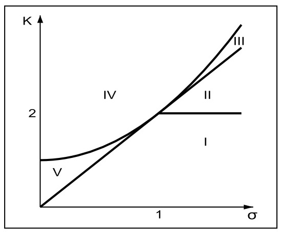
Figure 1: The phase diagram for system (7).

Since the main purpose of the work is an exact solution of equations (7), we omit the description of the standard qualitative analysis of the behavior of the system in the phase plane confining ourselves to the corresponding phase portraits (figures 2-6), and dwell on obtaining analytical expressions for the invariant manifolds.

To simplify analysis of system (7) and make results more intelligible we introduce the new variable

$$s=w+(\xi+\eta-1)r,$$ (8)

where the new parameters $\xi$ and $\eta$ are given by

$$\begin{array}[]{lcl}\xi&=&1-K/2+\sqrt{(K/2)^{2}-{\sigma}^{2}},\\[8.53581pt] \eta&=&1-K/2-\sqrt{(K/2)^{2}-{\sigma}^{2}}.\end{array}$$ (9)

Thus, we rewrite our system as

$$\left\{\begin{array}[]{lcl}\dot{r}&=&\left(\xi+\eta\right)r-s-r^{3},\\[8.53581pt] \dot{s}&=&\xi\eta r-r^{2}s\end{array}\right.$$ (10)

and will hereafter analyze the problem in the terms of $(r,s)$-variables.

Let us now consider the following quantity $\Gamma=\Gamma(r,s)$:

$$\Gamma=ar^{2}+bs^{2}-1.$$ (11)

By differentiating it and substituting the expressions for $\dot{r}$ and $\dot{s}$ from system (10) we get

$$\dot{\Gamma}=-2r^{2}[ar^{2}+bs^{2}-b\xi\eta(\xi+\eta)]-2(a-b\xi\eta)rs.$$ (12)

Choosing the parameters $a$ and $b$ as

$$a=\frac{1}{\xi+\eta},\qquad\qquad b=\frac{1}{\xi\eta(\xi+\eta)}$$ (13)

one can conclude that the evolution of quantity $\Gamma$ is governed by the simple equation:

$$\dot{\Gamma}=-2r^{2}\Gamma.$$ (14)

Thus, if at the initial moment of time the quantity $\Gamma_{0}=\Gamma(t=0)=0$, then it will be zero for all the values of $t$, which means that the second order curve

$$\frac{r^{2}}{\xi+\eta}+\frac{s^{2}}{\xi\eta(\xi+\eta)}=1$$ (15)

is an invariant manifold.

When the parameters $K$ and $\sigma$ belong to region I of the phase diagram the coefficients of (15) are positive and this second order curve, which is a stable limit cycle, is an ellipse. In such a way we have derived the explicit analytical expression describing the form of the limit cycle of our system (7).

As we move up along the line $\sigma=const>1$ (figure 1), the axes of the ellipse become smaller and smaller until at $K=2$ the limit cycle degenerates into the center, the $(0,0)$-point, which further transforms into the stable focus of region II. This phenomenon is the well-known Hopf bifurcation [17] and we would like to note that our system allows analytical description of this bifurcation, which is often not the case.

The line $K=2\sigma>2$ separates the regions with different types of the stable fixed point $(0,0)$: the stable focus of region II transforms into the stable node of region III. This line is actually not a bifurcation border from the view point of the dynamics of system (7), because the topology of its phase space is not changed.

One more well-known bifurcation, the pitchfork one, takes place at the boundary between regions III and IV: $K=\sigma^{2}+1>2$, where the stable node of region II looses its stability and transforms into the saddle (0,0) and two stable nodes $(\pm{\sqrt{\xi}},\mp{\eta\sqrt{\xi}})$ in region IV. In this region $\xi+\eta<0$, but $\xi\eta(\xi+\eta)>0$ and expression (15) describes a hyperbola.

Immediately after crossing the border between regions IV and V, in region V the saddle point $(0,0)$ transforms into the unstable node $(0,0)$ originating two saddles $(\pm{\sqrt{\eta}},\pm{\xi\sqrt{\eta}})$ while the stable nodes $(\pm{\sqrt{\xi}},\pm{\eta\sqrt{\xi}})$ remain. In region V both $\xi$ and $\eta$ are positive and line (15) is again an ellipse. However, contrary to region I, this ellipse now consists of four separatrices which start at the saddles $(\pm{\sqrt{\eta}},\pm{\xi\sqrt{\eta}})$ and end at the stable nodes $(\pm{\sqrt{\xi}},\pm{\eta\sqrt{\xi}})$. Thus, our simple calculations enabled us to establish the form of the separatrices (the parts of the ellipse).

While approaching to the boundary separating regions V and I, $K=2\sigma<2$, the angle between the straight-line invariant manifolds $s=\xi r$ and $s=\eta r$ decreases until, at the boundary, they merge into one unstable at the origin manifold $s=(1-\sigma)r$ along with the merging of the saddle and node points. This creates saddle-node points at the crossing with the ellipse. Further in region I the origin transforms into the unstable focus, the linear manifold disappears and the elliptic manifold becomes the limit cycle. At the border between regions IV and V the pairwise saddle-node or heteroclinic fold bifurcation [17] occurs.

Near the codimension-two point $\sigma=1,K=2$, where all the regions of the phase diagram of our two-dimensional system meet and the bifurcation borders cross, in high dimensional system (1) different dynamical regimes of the adjacent regions can mix. As was shown by the numerical study [8] in the phase diagram of the original system (1) near this point there is a region of unsteady dynamical behavior.

4 Analytical results

The main aim of this paper is stated as being the exact integration of system (7) or, with the use of the variables $r$ and $s$, system (10). The most straightforward way to do so consists of two steps. First, from (10) we can easy derive that the quantity $s/r$ satisfies a simple equation

$$\frac{d}{dt}\left(\frac{s}{r}\right)=\left(\frac{s}{r}-\xi\right)\left(\frac{s}{r}-\eta\right).$$ (16)

Looking at this equation one can immediately note that there are two stationary solutions $s/r=const$:

$$\frac{s}{r}=\xi,\qquad\qquad\frac{s}{r}=\eta$$ (17)

that correspond to the linear invariant manifolds represented in figures 4–6 (in the cases I and II parameters $\xi$ and $\eta$ are complex and these solutions do not any physical meaning).

Integrating equation (16) we can find that our variables $r$ and $s$ are related by

$$\frac{s}{r}=\frac{\eta E^{2}-\xi F_{0}}{E^{2}-F_{0}}$$ (18)

where

$$F_{0}=\frac{s_{0}-\eta r_{0}}{s_{0}-\xi r_{0}}$$ (19)

and

$$E^{2}=\exp{(\xi-\eta)t},$$ (20)

$s_{0},r_{0}$ are initial conditions of the problem.

The fact that the ratio $s/r$ satisfies the closed equation (16) which can be integrated explicitly makes it possible to reduce the order of our initial system and complete its solution. In some sense equation (18) plays the role of integral of motion (energy) in conservative systems.

To obtain $r$ and $s$ themselves we will present them in the following form:

$$r = u\left(\alpha E+\beta E^{-1}\right),$$ (21)

$$s = u\left(\alpha\eta E+\beta\xi E^{-1}\right).$$ (22)

Here $u=u(t)$ is a function that has to be found, the constants $\alpha$ and $\beta$, related by $\beta/\alpha=-F_{0}$, are determined by the initial conditions of the problem. This representation is a direct consequence of (18) which is rewritten in a more symmetric form convenient for the further analysis.

Substituting (21) and (22) into equation (10) and performing some algebraic transformations we arrive at the equation for the function $u(t)$:

$${\frac{du}{dt}=\frac{\xi+\eta}{2}u-{\left(\alpha E+\beta E^{-1}\right)}^{2}u^{3}}.$$ (23)

This equation is the so-called Abel equation of the first kind [18]. Using the substitution

$$u=v^{-1/2}$$ (24)

one can convert (23) into the linear equation

$${\frac{d}{dt}v}+(\xi+\eta)v=2{\left(\alpha E+\beta E^{-1}\right)^{2}}.$$ (25)

The solution of this equation is

$$v=v_{*}e^{-(\xi+\eta)t}+\displaystyle{\frac{\alpha^{2}}{\xi}e^{(\xi-\eta)t}+\frac{\beta^{2}}{\eta}e^{(\eta-\xi)t}+\frac{4\alpha\beta}{\xi+\eta}},$$ (26)

where the constant $v_{*}$ should be determined from the initial conditions. That gives

$$v_{*}=1-\displaystyle{\frac{\alpha^{2}}{\xi}-\frac{\beta^{2}}{\eta}-\frac{4\alpha\beta}{\xi+\eta}}$$ (27)

and

$$\alpha=\displaystyle{\frac{s_{0}-\xi r_{0}}{\eta-\xi}},$$ (28)

$$\beta=-\displaystyle{\frac{s_{0}-\eta r_{0}}{\eta-\xi}}.$$ (29)

Here we assumed without breaking the generality of the solution that $u(t=0)={v_{0}}^{-1/2}=1$ (for a system of two ordinary differential equations of the first order we need just two arbitrary constants).

Thus, we have integrated our nonlinear problem and expressions (21), (22) together with (26)-(29) give us its complete analytical solution. As one can see, the obtained solution has quite a compact form convenient for analysis.

5 Analysis of the results

In this section we continue the description of the system behavior started in section 3. Before proceeding further let us note that substituting (28) and (29) into (27) we can rewrite the constant $v_{*}$ as

$$v_{*}=1-\frac{r_{0}^{2}}{\xi+\eta}-\frac{s_{0}^{2}}{\xi\eta(\xi+\eta)}=-\Gamma_{0}.$$ (30)

It turns out that $v_{*}$ is nothing but? up to the sign¡ the quantity $\Gamma_{0}$ introduced in section 3. So, the constant $v_{*}$ indicates how far the initial point is from the invariant manifold $\Gamma=0$ at the initial moment.

Now let us consider the solution of the system in regions I and II of the phase diagram. The common feature of these regions is that the parameters $\xi$ and $\eta$ are complex: $\xi=\bar{\eta}$, and the constants $\alpha$ and $\beta$ are related as $\alpha=\bar{\beta}$. In this case the solution of the system can be presented as

$$r = 2\frac{|\alpha|}{\sqrt{v}}\cos(\xi^{\prime\prime}t+\phi_{\alpha}),$$ (31)

$$s = 2\frac{|\alpha||\xi|}{\sqrt{v}}\cos(\xi^{\prime\prime}t+\phi_{\alpha}-\phi_{\xi})$$ (32)

and

$$v=v_{*}e^{-2\xi^{\prime}t}+2\frac{|\alpha|^{2}}{|\xi|}\cos(2\xi^{\prime\prime}t+2\phi_{\alpha}-\phi_{\xi})+2\frac{|\alpha|^{2}}{\xi^{\prime}},$$ (33)

where the following notations are introduced: $\xi=\xi^{\prime}+i\xi^{\prime\prime}$, $\phi_{\alpha}=\arg\alpha$, $\phi_{\xi}=\arg\xi$ .

Now it is easy to see that in the first region, where Re $\xi$ = Re $\eta>0$, the exponential term in $v$ vanishes as $t\to\infty$ for arbitrary initial conditions and the solution becomes periodic which corresponds to the movement along the limit cycle.

The movement along the limit cycle is described by (31), (32) and (33) with $v_{*}=-\Gamma_{0}=0$. The period of circulation along the cycle is

$$T=\frac{2\pi}{\xi^{\prime\prime}}.$$ (34)

The plots $r=r(t)$ in figure 2 (Ib) present two typical solutions with initial conditions corresponding to the points of the phase portrait lying inside and outside the limit cycle. These solutions fit the so-called ‘large oscillations’ which were found numerically in the previous works [9, 10].

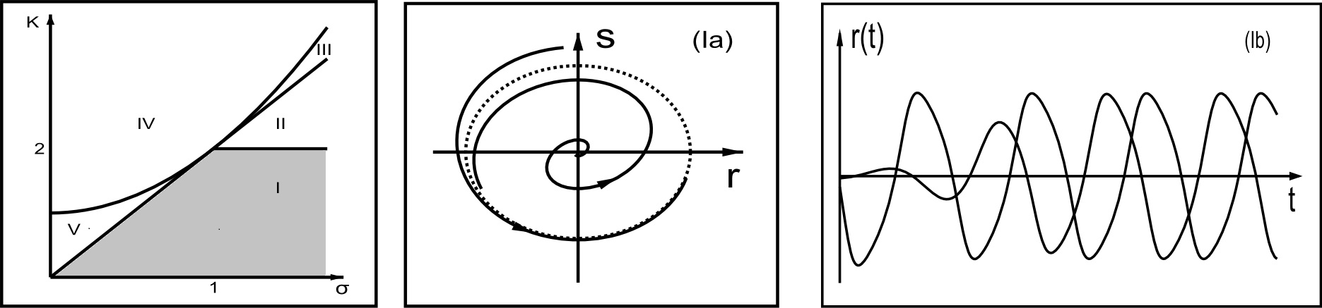
Figure 2: Typical phase trajectories (in the middle) and the evolution of the centroid amplitudes (on the right) corresponding to region I of the phase diagram (on the left) for different initial conditions. The limit cycle is plotted with dotted lines.

For parameter values in region II Re $\xi$ = Re $\eta<0$, the exponent in (33) tends to infinity at $t\to\infty$ and our solutions, having a periodic component, tends to the point of the stable focus (0,0) (figure 3 (IIb)).

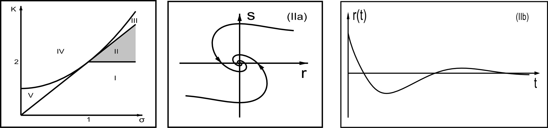
Figure 3: Typical phase trajectories and the evolution of of the centroid amplitude corresponding to region II of the phase diagram.

A similar asymptotic behavior is observed in case III: for all the initial conditions $\lim\limits_{t\to\infty}r=\lim\limits_{t\to\infty}s=0$. The difference is that now we do not have oscillations. This is a manifestation of the fact that the stable point $(0,0)$ is the stable node and not the focus as in case II (see Fig. 4). Both the second and the third cases correspond to the amplitude death of [9, 10] when oscillations are quenched and the system evolves to the stable equilibrium.

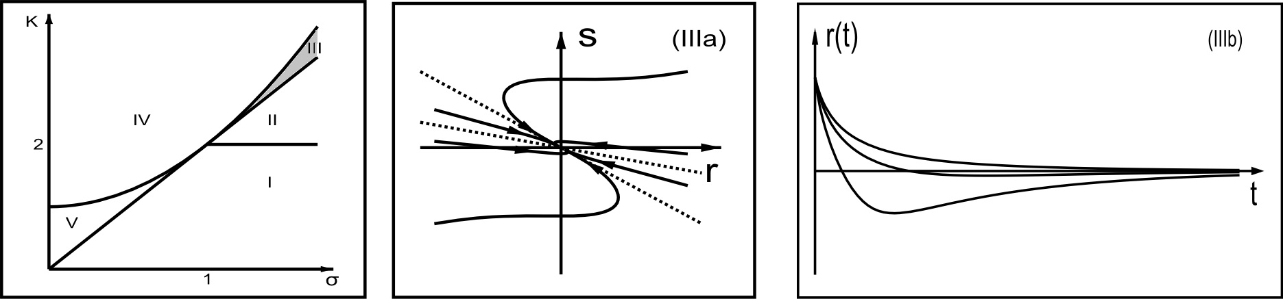
Figure 4: Typical phase trajectories and the evolution of amplitudes of the centroid for region III of the phase diagram; the invariant manifolds are plotted with dotted lines.

In the case IV expressions (26)-(29) describe the phase-locked solutions of our system when asymptotically the population as a whole starts oscillate with the common amplitude $r^{2}=\xi$ (see figure 5 (IVb)).

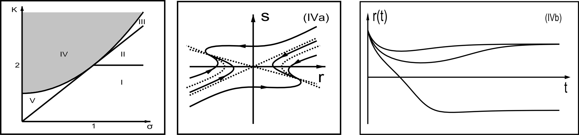
Figure 5: Typical phase trajectories and the evolution of the centroid amplitudes for region IV of the phase diagram; the invariant manifolds are plotted with dotted lines.

For the parameter values of region V of the phase diagram the solutions of system (7) are presented in figure 6. Though the asymptotic behavior of our system in the cases IV and V is visually similar these cases correspond to different geometry of their phase portraits which can be essential in more elaborated descriptions.

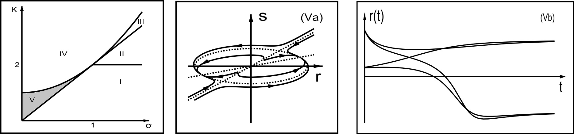
Figure 6: Phase portraits and typical evolution of amplitude $r=r(t)$ corresponding to region V of the phase diagram; the invariant manifolds are plotted with dotted lines.

6 Conclusion.

In this paper we have integrate exactly the nonlinear system (7) describing the evolution of macroscopic order parameters, mean field (2) and the amplitude-phase correlator (3), of the ensemble of $N$ nonidentical globally coupled Stuart-Landau oscillators (1). Expressions (21), (22) and (26)-(29) represent the complete analytical solution of system (4) on the two-dimensional invariant manifold where the order parameters are orthogonal. We present a complete classification of phase portraits and bifurcations, obtain explicit expressions for invariant manifolds and derive analytical solutions for arbitrary initial data and different regimes. The obtained results confirm the qualitative and numerical description of (7) offered in [10] and lead us to expect that analytical solutions can also be found in a less restricted situation, which will be the subject of future studies.

References

- [1] Kuramoto Y 1984 Chemical Oscillations, Waves and Turbulence (Berlin: Springer)
- [2] Strogatz S H 2003 Sync: The Emerging Science of Spontaneous Order (Hyperion, New York)
- [3] Strogatz S H 2014 Nonlinear Dynamics and Chaos: With Applications to Physics, Biology, Chemistry, and Engineering, 2nd edition (Westview Press, Boulder)
- [4] Pikovsky A, Rosenblum M and Kurths J 2001 Synchronization (Cambridge: Cambridge University Press)
- [5] Acebron J A, Bonilla L L, Perez Vicente C J, Ritort F, Spigler R, 2005 The Kuramoto model: a simple paradigm for synchronization phenomena. Rev. Mod. Phys. 77 137-185.
- [6] A. Pikovsky and M. Rosenblum 2015 Dynamics of globally coupled oscillators: progress and perspectives arXiv:1504.06747 [nlin.AO]
- [7] Kuramoto Y, 1975, International Symposium on Mathematical Problems in Theoretical Physics, Lecture Notes in Physics, Vol. 39 ed H Arakai (Springer, New York)
- [8] Mattews P C, Mirollo R E and Strogatz S H 1991 Dynamics of a large system of coupled nonlinear oscillators Physica D 52 293-331
- [9] Matthews P C and Strogatz S H 1990 Phase diagram for the collective behavior of limit-cycle oscillators Phys. Rev. Lett. 65 1701-04
- [10] De Monte S, d’Ovidio F 2002 Dynamics of order parameters for globally coupled oscillators Europhys. Lett. 58 121-127
- [11] De Monte S, d’Ovidio F, Mosekilde E 2003 Coherent regimes of globally coupled dynamical systems Phys. Rev. Lett. 90 054202
- [12] De Monte S, d’Ovidio F, Chaté H, and Mosekilde E 2004 Noise-induced macroscopic bifurcations in globally-coupled chaotic units Phys. Rev. Lett. 92 254101
- [13] De Monte S, d’Ovidio F, Chaté H, and Mosekilde E 2005 Effects of Microscopic Disorder on the Collective Dynamics of Globally Coupled Maps Physica D: Nonlinear Phenomena 205 25
- [14] Gomes Da Silva I, De Monte S, d’Ovidio F, Toral R, and Mirasso C R 2006 Coherent regimes of mutually coupled Chua’s circuits Phys. Rev. E 73 036203
- [15] Komin N and Toral R 2010 Phase transitions induced by microscopic disorder: A study based on the order parameter expansion Physica D: Nonlinear Phenomena 239 1827
- [16] Komin N and Toral R 2010 Order parameter expansion and finite-size scaling study of coherent dynamics induced by quenched noise in the active rotator model Phys. Rev. E 82 051127
- [17] Kuznetsov Y A 1998 Elements of Applied Bifurcation Theory, 2nd ed. (New York: Springer-Verlag)
- [18] Zwillinger D 1997 Handbook of Differential Equations, 3rd ed. (Boston: Academic Press)