Remarkable analytic relations among greybody parameters

Abstract

In this paper we derive and discuss several implications of the analytic form of a modified blackbody, also called greybody, which is widely used in Astrophysics, and in particular in the study of star formation in the far-infrared/sub-millimeter domain. The research in this area has been greatly improved thanks to recent observations taken with the Herschel satellite, so that it became important to clarify the sense of the greybody approximation, to suggest possible further uses, and to delimit its intervals of validity. First, we discuss the position of the greybody peak, making difference between the optically thin and thick regimes. Second, we analyze the behavior of bolometric quantities as a function of the different greybody parameters. The ratio between the bolometric luminosity and the mass of a source, the ratio between the so-called “sub-millimeter luminosity” and the bolometric one, and the bolometric temperature are observables used to characterize the evolutionary stage of a source, and it is of primary importance to have analytic equations describing the dependence of such quantities on the greybody parameters. Here we discuss all these aspects, providing analytic relations, illustrating particular cases and providing graphical examples. Some equations reported here are well-known in Astrophysics, but are often spread over different publications. Some of them, instead, are brand new and represent a novelty in Astrophysics literature. Finally we indicate an alternative way to obtain, under some conditions, the greybody temperature and dust emissivity directly from an observing spectral energy distribution, avoiding a best-fit procedure.

1 Introduction

The concept of blackbody is widely used in modern Astrophysics to model a quantity of phenomena that approach the ideal case of radiation emitted by an object at the thermal equilibrium which is a perfect emitter and absorber; the shape of the spectrum is completely described in terms of its temperature. Laws describing global characteristics of the blackbody, as the Wien’s or of Stefan-Boltzmann’s ones, represent renowned milestones of quantum Physics. However, as far as the continuum emission of a source departs from a perfect blackbody behavior and another analytic expression is invoked in place of the Planck’s function to describe the corresponding spectral energy distribution (hereafter SED), it becomes interesting to understand how the well-known relations valid for a blackbody have to change in turn.

In particular, large and cold interstellar dust grains ($D>0.01~{}\mu$m, $T\lesssim 20$ K) are recognized to be poor radiators at long wavelengths ($\lambda\gtrsim 50~{}\mu$m), therefore their emission requires to be modeled by a blackbody law with a modified emissivity smaller than 1 (i.e. the value corresponding to the ideal case), and being a decreasing function of wavelength (see, e.g., Gordon, 1995, and references therein). The typically adopted expressions for such emissivity are summarized in Section 2 of this paper.

Modeling the dust emission with a modified blackbody (hereafter greybody for the sake of brevity) has been widely used to obtain the surface density and (if distance is known) the total mass along the line of sight for structures in the Milky Way (diffuse clouds, filaments, clumps, cores) or for entire external galaxies. Two cases are generally possible: $i)$ an observed SED is available, built with at least three spectral points, so that a best-fit is performed to determine simultaneously both the column density and the average temperature of the emitting source (e.g., André et al., 2000; Olmi et al., 2009), or $ii)$ only one flux measurement at a single wavelength (typically in the sub-millimeter regime) is available, then an assumption on the temperature value has to be made (e.g., Faúndez et al., 2004; Mookerjea et al., 2007) to obtain the column density.

Recently, the availability of large amounts of data from large survey programs for the study of star formation with the Herschel satellite (Pilbratt et al., 2010), such as Hi-GAL (Molinari et al., 2010), HGBS (André et al., 2010), HOBYS (Motte et al., 2010), and EPoS (Ragan et al., 2012) made it possible to build the far-infrared/sub-millimeter five band (70, 160, 250, 350, and 500 $\mu$m) SEDs of the cold dust in the Milky Way (e.g., Elia et al., 2010; Könyves et al., 2010; Giannini et al., 2012; Pezzuto et al., 2012; Elia et al., 2013) in a crucial range usually containing the emission peak of cold dust. In this case the approach described at the point $i$ represents the preferable way for estimating the physical parameters of the greybody which best approaches the observed SED.

In this paper, after introducing in Section 2 the analytic expression of the greybody, in Section 3 we discuss how, unlike the case of a blackbody, the position of the greybody emission peak shifts as a function of different parameters besides the temperature. Moreover, further obtainable quantities as, for example, bolometric luminosity and temperature, are often used to characterize star forming clumps (e.g., Elia et al., 2010, 2013; Giannini et al., 2012; Strafella et al., 2015). A comparison with the values predicted analytically by the greybody model as a function of its physical parameters turn out to be interesting in this respect. We derive such functional relationships in Sections 4 and 5. Further considerations on the obtained analytic relations suggest a method for deriving the greybody temperature and dust emissivity of an SED without carrying out a best-fit procedure. This is discussed in Section 6. Finally, in Section 7 we summarize the obtained results.

2 The equation of a greybody

The solution of the radiative transfer equation for a medium with optical depth $\tau_{\nu}$ (function of the observed frequency $\nu$) and for a source function constituted by the Planck’s blackbody $B_{\nu}$ at temperature $T$ is

$$I_{\nu}=(1-\mathrm{e}^{-\tau_{\nu}})\,B_{\nu}(T)$$ (1)

(cf., e.g., Choudhuri, 2010), where

$$B_{\nu}(T)=\frac{2\,h\,\nu^{3}}{c^{2}}\frac{1}{\mathrm{e}^{\frac{h\,\nu}{k_{B}\,T}}-1}\,.$$ (2)

With $h$, $k_{B}$, and $c$ we indicate the Planck’s and Boltzmann’s constants and the light speed in vacuum, respectively. Assuming $I_{\nu}$ being uniform over the solid angle $\Omega$, the corresponding flux is

$$F_{\nu}=\Omega\,(1-\mathrm{e}^{-\tau_{\nu}})\,B_{\nu}(T)\,.$$ (3)

The empirical behavior of $\tau_{\nu}$ as a function of $\nu$ for large interstellar dust grains is generally modeled as a power law (Hildebrand, 1983) with exponent $\beta$:

$$\tau_{\nu}=\left(\frac{\nu}{\nu_{0}}\right)^{\beta}\,,$$ (4)

where the parameter $\nu_{0}$ is such that $\tau_{\nu_{0}}=1$.

In the limit of $\nu\ll\nu_{0}$, the term $(1-\mathrm{e}^{-\tau_{\nu}})$ can be approximated as follows

$$\lim_{\frac{\nu}{\nu_{0}}\rightarrow 0}\left(1-\mathrm{e}^{-\tau_{\nu}}\right)=\tau_{\nu}=\left(\frac{\nu}{\nu_{0}}\right)^{\beta}\,.$$ (5)

For an opportunely large $\nu_{0}$ it can happen that all the observed frequencies fall in the regime in which the greybody turns out to be optically thin. In such case, Equation (1) becomes

$$I_{\nu}\approx\left(\frac{\nu}{\nu_{0}}\right)^{\beta}B_{\nu}(T)\,.$$ (6)

Recalling the definition of optical depth, $\tau_{\nu}\equiv\kappa_{\nu}\int\rho\mathrm{d}s$, where $\kappa_{\nu}$ is the opacity of the medium, $\rho$ is its volume density and $s$ is the spatial integration variable along the line of sight, in the optically thin regime it becomes

$$\tau_{\nu}\approx\kappa_{\mathrm{ref}}\left(\frac{\nu}{\nu_{\mathrm{ref}}}\right)^{\beta}\Sigma,$$ (7)

where $\Sigma$ is the surface, or column, density, and $\kappa_{\mathrm{ref}}$ is the opacity estimated at a reference frequency $\nu_{\mathrm{ref}}$. For an optically thin envelope, $\Sigma=M/A$ where $M$ is the mass and $A$ is the projected area of the source. For a source located at distance $d$, $A=\Omega\,d^{2}$, so $\Omega=M/(\Sigma\,d^{2})=(M\,\kappa_{\mathrm{ref}})/(\tau\,d^{2})$, then Equation 3 becomes

$$F_{\nu}=\frac{M\,\kappa_{\mathrm{ref}}}{d^{2}}\,\left(\frac{\nu}{\nu_{\mathrm{ref}}}\right)^{\beta}\,B_{\nu}(T)\,.$$ (8)

The decision whether the optically thin assumption is valid or not depends on the validity of the substitution $\tau$ for $(1-\mathrm{e}^{-\tau})$. In turn, this means that the error $\left|[\tau-(1-\mathrm{e}^{-\tau})]/[1-\mathrm{e}^{-\tau}]\right|$ should be negligible compared to the data uncertainties. This point is almost always overlooked in the literature. Notice that if $\tau=0.2$ the error introduced in the mathematical substitution is 10%, which is negligible only if the fluxes have been measured with a much larger uncertainty. When $\tau=0.1$ the error is $\sim$5% and only when $\tau=0.02$ the error becomes of the order of 1%.

Finally, let us remind the reader that so far we expressed all quantities as functions of $\nu$, but they can be equivalently formulated in terms of the wavelength $\lambda$. For example, the optical depth can be expressed also as $\tau=(\lambda/\lambda_{0})^{-\beta}$, with $\lambda_{0}=c/\nu_{0}$. Furthermore, in the literature regarding dust emission in the far infrared/sub-millimeter, generally one encounters the quantity $B_{\nu}(T)$, measured in Jy/sr, expressed as a function of $\lambda$ (in $\mu$m), which the reader has to keep in mind before applying the equations reported in this paper to specific cases.

3 The maximum of greybody emission

The peak position of $I_{\nu}$ can be found by differentiating Equation 1 with respect to $\nu$. Nevertheless, we prefer to start from the optically thin case (Equation 6), which is quite simpler, and can be approached in a way similar to the derivation of the Wien’s displacement law for a blackbody. In this latter case, imposing the derivative of the Planck’s function to be 0 leads to solve numerically the equation (see, e.g., Rybicki & Lightman, 1979)

$$x=3(1-\mathrm{e}^{-x})\,,$$ (9)

where $x\equiv h\,\nu/k_{B}\,T$. The solution of this equation is $x\simeq 2.82$, i.e. $\nu_{\mathrm{b}}/T=5.88\times 10^{10}$ Hz K^-1.

Similarly, imposing the same condition to the expression in Equation 6, the equation to be solved becomes

$$x=(3+\beta)(1-\mathrm{e}^{-x})\,,$$ (10)

which for $\beta=0$ corresponds to Equation 9. The value of $x$ increases with $\beta$: for instance $x=3.92$ for $\beta=1$, and $x=4.97$ for $\beta=2$. This means that for any $\beta\geq 1$ putting $1-\mathrm{e}^{-x}$ equal to 1 results in an error smaller than 2%. So we can write

$$x\simeq 3+\beta$$ (11)

or

$$\nu_{\mathrm{p}}\simeq\frac{k_{B}\,T\,(3+\beta)}{h}=20.837\,T\,(3+\beta)\,\,\,[\mathrm{GHz}]\,.$$ (12)

The corresponding wavelength is given by

$$\lambda_{\nu_{\mathrm{p}}}\simeq\frac{hc}{k_{B}\,T(3+\beta)}=\frac{1.439}{T(3+\beta)}\,\,\mathrm{cm}\,.$$ (13)

Let us remind the reader that this is the wavelength at which the peak of $I_{\nu}$ is encountered, so Equation 13 does not apply to $I_{\lambda}$ (see below). In Figure 1, $I_{\nu}$ as a function of $\lambda$ is shown for different values of $T$ and $\beta$, highlighting how the peak position varies according to Equation 10.

Similarly to Equation 9, the peak wavelength of $I_{\lambda}$ has to be calculated starting from

$$\frac{\partial}{\partial\lambda}\left[\left(\frac{\lambda}{\lambda_{0}}\right)^{-\beta}B_{\lambda}(T)\right]=0\,,$$ (14)

which, leads to an equation like

$$x=(5+\beta)(1-\mathrm{e}^{-x})\,,$$ (15)

where $x\equiv h\,c/\lambda\,k_{B}\,T$ in this case. From this equation, for $\beta=0$, one can obtain the most used formulation of the Wien’s displacement law, the one in terms of $I_{\lambda}$ and $\lambda_{\mathrm{p}}$. Since Equations 10 and 15 constitute an incompatible system, this gives an alternative demonstration of the known result $\lambda_{\mathrm{p}}\neq\lambda_{\nu_{\mathrm{p}}}$, namely the wavelengths at which $I_{\lambda}$ and $I_{\nu}$ peak, respectively, do not coincide.

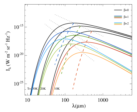
Figure 1: Plot of $I_{\nu}$ as a function of $\lambda$ for different values of parameters $T$ and $\beta$, in the optically thin case, described by Equation 6. Three temperatures are probed: 10, 20, and 30 K, corresponding to three sets of curves (red, green, and blue, respectively); for each temperature, three values of $\beta$ are probed: 0 (corresponding to the case of a blackbody), 1, and 2, which are plotted, for each set of curves, in black, dark color and light color. The frequency $\nu_{0}$ is chosen such that $\lambda_{0}=5~{}\mu$m, in order to fulfill the requirements of the optically thin approximation in the considered range of wavelengths. Dashed lines connect maxima of $I_{\nu}$ at different $\beta$ values, from 0 (top) to 6 (bottom), at $T=10$ (red), 20 (green), and 30 K (blue), respectively. Grey dotted lines, instead, connect maxima of $I_{\nu}$ at different temperatures, for the cases $\beta=0$ (top), 1 (middle), and 2 (bottom). All the three lines start at $T=100$ K (top left) down to $T=5$ K (bottom right).

Let us now consider the most general case. Again, the derivative of $I_{\nu}$ with respect to $\nu$ is easier to compute. First of all, let us notice that

$$\frac{\partial(1-\mathrm{e}^{-\tau_{\nu}})}{\partial\nu}=\frac{\beta\tau_{\nu}\mathrm{e}^{-\tau_{\nu}}}{\nu}\,.$$ (16)

Therefore,

$$\begin{split}&\frac{\partial}{\partial\nu}\left[(1-\mathrm{e}^{\tau_{\nu}})B_{\nu}(T)\right]=0\,\Rightarrow\\ &\Rightarrow\frac{2\,h\,\nu^{2}}{c^{2}}\frac{1}{\mathrm{e}^{\frac{h\,\nu}{k_{B}\,T}}-1}\times\\ &\times\left[\beta\tau_{\nu}\mathrm{e}^{-\tau_{\nu}}+(1-\mathrm{e}^{-\tau_{\nu}})\left(3-\frac{h\nu}{k_{B}\,T}\frac{\mathrm{e}^{\frac{h\nu}{k_{B}\,T}}}{\mathrm{e}^{\frac{h\nu}{k_{B}\,T}}-1}\right)\right]=0\,.\end{split}$$ (17)

Using again $x\equiv h\,\nu/k_{B}\,T$, the last condition is satisfied if

$$\frac{\beta\tau_{\nu}}{\mathrm{e}^{\tau_{\nu}}-1}=\frac{x}{1-\mathrm{e}^{-x}}-3\,.$$ (18)

In the above equation, when $\nu\rightarrow 0$ the two fractions tend to $\beta$ and 1, respectively; so the right hand side tends to -2. When $\nu\gg 1$ the left hand side tends to 0, while the right hand side tends to $x-3$. Since the left hand side is always positive, the solution $\nu_{\mathrm{p}}$ of the equation must be greater than the frequency $\nu_{\mathrm{b}}$ at which the right hand becomes positive (notice that $\nu_{\mathrm{b}}$, defined in this way, coincides with the solution of Equation 9, which is valid in the case of a pure blackbody).

In Figure 2 the two sides of Equation 18 are plotted vs the frequency, in correspondence of different choices of the parameters $\beta$, $\nu_{0}$, and $T$. It is noteworthy that the left hand side of the equation depend only on the first two of these parameters, while the right hand side depends only on the third one. In this figure one can find a graphical representation of the $\nu_{\mathrm{p}}>\nu_{\mathrm{b}}$ condition.

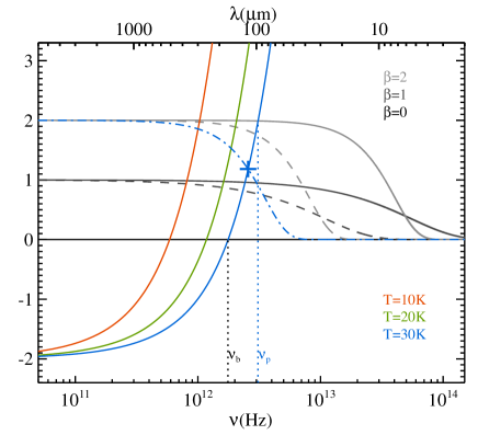
Figure 2: The two sides of Equation 18 plotted as a function of frequency (bottom $x$-axis) and wavelength (top $x$-axis). Units on the $y$-axis are adimensional numbers. Grey lines represent the left hand side for $\beta=0$ (black), 1 (dark grey), and 2 (light grey), respectively, with $\nu_{0}=30$ THz (solid lines) and $\nu_{0}=6$ THz (dashed lines), corresponding to $\lambda_{0}=10$ and $50~{}\mu$m, respectively. In addition, the case $\beta=2$ and $\nu_{0}=\nu_{\mathrm{p}}$ at $T=30~{}\mathrm{K}$, namely $\nu_{0}=2.6$ GHz, (obtained through Equation 21) is plotted as a blue dotted-dashed curve. The red, green and blue solid curves represent the right hand side for T=10, 20, and 30 K, respectively. For a given choice of the parameters $\beta$, $\nu_{0}$, and $T$, the abscissae of the intersections of the colored curves with the grey ones represent the solutions $\nu_{\mathrm{p}}$ of Equation 18, while the intersections with the black curve represent the blackbody case ($\nu_{\mathrm{b}}$). The fact that $\nu_{\mathrm{p}}>\nu_{\mathrm{b}}$ is highlighted in the case of $T=30$ K through two vertical dotted lines at the positions of $\nu_{\mathrm{b}}$ (black) and $\nu_{\mathrm{p}}$ at $\beta=2$ (blue). The intersection between the two blue lines, i.e. the solid and the dotted-dashed one, is marked with a blue cross and is discussed in the text.

Note that in the limiting case $\nu_{0}\rightarrow 0$ (a greybody optically thick at all frequencies) one obtains $\nu_{\mathrm{p}}\rightarrow\nu_{\mathrm{b}}$.

The opposite limiting case is $\nu_{0}\rightarrow\infty$ (a greybody optically thin at all frequencies), in which the left hand side of Equation 18 gets constantly equal to $\beta$ and the frequency of the peak corresponds to the solution of Equation 12.

In summary, combining Equations 12 and 18 one finds

$$1<\nu_{\mathrm{p}}/\nu_{\mathrm{b}}\leq\left\{\begin{tabular}[]{cc}1.43&$\beta=1$\\ 1.79&$\beta=2$\\ 2.14&$\beta=3$\end{tabular}\right.$$ (19)

So, even though $\nu_{0}$ can be any real number, nonetheless the peak frequency of the greybody lies within a limited range of values that can be parametrized in terms of the peak frequency of the blackbody.

We can go further on in extracting information from Equation 18, which gives the peak of the greybody for any given set of the three parameters $\nu_{0}$, $T$, and $\beta$. However, if the peak is fixed to the frequency $\nu_{\mathrm{p}}$, then only two parameters remain free. If we also impose the condition $\nu_{\mathrm{p}}=\nu_{0}$, equivalent to assume $\tau_{\nu_{\mathrm{p}}}=1$, only one parameter is left free, and Equation 18 becomes

$$\frac{\beta}{\mathrm{e}-1}=\frac{x}{1-\mathrm{e}^{-x}}-3\,,$$ (20)

which, for any chosen $\nu_{\mathrm{p}}$, gives the relation between $T$ and $\beta$: if one fixes, say, $T$, then Equation 20 gives the value of $\beta$ such that $\nu_{0}=\nu_{\mathrm{p}}$, and vice versa. We give a graphical example of this for $T=30$ K and $\beta=2$ in Figure 2, highlighting $\nu_{\mathrm{p}}=\nu_{0}$ with a blue cross.

The numerical solutions of Equation 20 are $x=3.47,4.10,4.70$ for $\beta=1,2,3$, respectively. With these values for $x$, it is possible to put $x/\left[1-\mathrm{e^{-x}}\right]\simeq x$. The error decreases from 3% for $\beta=1$ to less than 1.1% for $\beta=3$. So, for $\tau_{\nu_{\mathrm{p}}}=1$,

$$\nu_{\mathrm{p}}=\frac{k_{B}\,T}{h}\left(\frac{\beta}{\mathrm{e}-1}+3\right)\,.$$ (21)

In the above form, Equation 21 gives, for any pair ($T,\beta$), the frequency of the peak of a greybody such that $\tau_{\nu_{\mathrm{p}}}=1$; for instance, when $T=10$ K one finds $\nu_{0}=746,868,989$ GHz (in terms of wavelengths, $\lambda_{0}=402,346,303~{}\mu$m) for $\beta=1,2,3$, respectively. For other temperatures, note that $\nu_{0}$ scales linearly with $T$. Now we invert the problem: we fix $\lambda_{0}$ and $\beta$ and look for the values of $T$ that make the peak of the greybody falling at $\lambda_{\mathrm{p}}=\lambda_{0}$. Dealing, for example, with Herschel, it is natural to set $\lambda_{0}=70~{}\mu$m. Then we find $T=57$ K for $\beta=1$, and $T=43$ K for $\beta=3$. So, the triple ($\lambda_{0}=70~{}\mu$m, $T=43$ K, $\beta=3$) is such that $\lambda_{\mathrm{p}}=\lambda_{0}$ and then $\tau(\lambda=70\mu\mathrm{m})=1$. If we keep constant $\lambda_{0}$ and consider $T\leq 43$ K and $\beta\leq 3$, then the wavelength of the peak shifts to $\lambda_{\mathrm{p}}>\lambda_{0}$ (e.g., for $\lambda=70$ $\mu$m, $T=40$ K and $\beta=2.5$ from Equation 18 we find $\lambda_{\mathrm{p}}\sim~{}78$ $\mu$m) so that $\tau_{\nu_{\mathrm{p}}}=(\nu_{\mathrm{p}}/\nu_{0})^{\beta}<1$. In conclusion, as long as the temperature of the greybody is less than 43 K (the typical case encountered in recent Herschel literature, e.g., Giannini et al., 2012; Elia et al., 2013) we are sure that $\tau_{\nu_{\mathrm{p}}}\leq 1$, independently of the values of $T,\beta$ and, for $\lambda_{0}\leq 70~{}\mu$m, of $\nu_{0}$, as long as $\beta\leq 3$.

The main limitation of this conclusion is that, actually, it does depend on $\nu_{0}$ which, in general, is not known even if the sources observed with Herschel typically have $\lambda_{0}\lesssim 70~{}\mu$m. In any case, to go further also when only $T$ and $\beta$ are known we proceed as follows: first we note that if $\tau_{\nu_{\mathrm{p}}}<1$ then $\tau_{\nu_{\mathrm{p}}}/(\mathrm{e}^{\tau_{\nu_{\mathrm{p}}}}-1)>0.582$ (this ratio tends to 1 for $\tau_{\nu_{\mathrm{p}}}\rightarrow 0$). This condition implies that

$$\frac{1}{\beta}\left(\frac{x_{\mathrm{p}}}{1-\mathrm{e}^{-x_{\mathrm{p}}}}-3\right)>0.582\Rightarrow\frac{x_{\mathrm{p}}}{1-\mathrm{e}^{-x_{\mathrm{p}}}}>\frac{\beta}{\mathrm{e}-1}+3\,.$$ (22)

For $\beta=1$, $x_{\mathrm{p}}\gtrsim 3.58$, whilst for $\beta=3$, $x_{\mathrm{p}}\gtrsim 4.70$; with these values of $x_{\mathrm{p}}$ one can assume $1-\mathrm{e}^{-x_{\mathrm{p}}}\simeq 1$, the error being about 3% for $\beta=1$ and even lower for higher $\beta$. So, under the condition $\tau_{\nu_{\mathrm{p}}}<1$, we can cast Equation 21 in the form

$$x_{\mathrm{p}}=\frac{h\,c}{k_{\mathrm{B}}\,\lambda_{\mathrm{p}}\,T}>\frac{\beta}{\mathrm{e}-1}+3\,,$$

then, finally,

$$\lambda_{\mathrm{p}}<\frac{h\,c}{k_{\mathrm{B}}\,T}\frac{\mathrm{e}-1}{\beta+3(\mathrm{e}-1)}\,.$$ (23)

This result can be clearly seen in Figure 2, where the blue cross symbol represents the right hand side of Equation 23 for $T=30$ K and $\beta=2$. All family of curves representing the left hand side of Equation 18 intersecting, in this case ($T=30$ K), the blue solid curve below the cross symbol have $\tau_{\nu_{\mathrm{p}}}>1$ and ${\lambda_{\mathrm{p}}}$ violating the condition imposed in Equation 23. Clearly, varying the temperature would change the position of the cross symbol in that diagram.

If we use Equation 6 to fit a SED known over a set of fluxes at wavelengths longer than a certain $\lambda_{\mathrm{min}}$, to obtain a reliable estimate of $T$ it should be that $\lambda_{\mathrm{p}}>\lambda_{\mathrm{min}}$; if this is the case, the condition to have $\tau_{\nu_{\mathrm{p}}}<1$ becomes

$$\lambda_{\mathrm{min}}<\frac{h\,c}{k_{\mathrm{B}}\,T}\frac{\mathrm{e}-1}{\beta+3(\mathrm{e}-1)}\,.$$ (24)

Solving for $T$ and setting, for example, $\lambda_{\mathrm{min}}=70$ $\mu$m we obtain $T\lesssim 45$ K for $\beta\leq 3$; but $T\lesssim 31$ K is found for $\lambda_{\mathrm{min}}=100$ $\mu$m and $T\lesssim 20$ K for $\lambda_{\mathrm{min}}=160$ $\mu$m.

A couple of comments can be made: first, if one uses Equation 13 to find the peak of the greybody, then Equation 24 is always verified. This happens because Equation 13 is valid if $\tau_{\nu_{\mathrm{p}}}\ll 1$ while Equation 24 is more general, having imposed only that $\tau_{\nu_{\mathrm{p}}}<1$. Second, the condition $\tau_{\nu_{\mathrm{p}}}<1$ means that $\lambda_{0}<\lambda_{\mathrm{p}}$; the assumption $\lambda_{\mathrm{min}}<\lambda_{\mathrm{p}}$ does not imply that $\lambda_{0}<\lambda_{\mathrm{min}}$, so that Equation 24 gives a necessary but not sufficient condition to justify the use of Equation 6. In other words, the relation $\lambda_{\mathrm{min}}<\lambda_{0}<\lambda_{\mathrm{p}}$ is compatible with Equation 23 and in this case it is still true that $\tau_{\nu_{\mathrm{p}}}<1$; but then there is a portion of the SED, between $\lambda_{\mathrm{min}}$ and $\lambda_{0}$, where $\tau_{\nu}>1$ so that the use of Equation 6 is not justified over the whole observed SED.

We conclude this section by noting that Equation 24 is a condition to have $\tau_{\nu_{\mathrm{p}}}<1$, not a condition to have a reliable fit of the SED: if the peak falls at wavelengths shorter than $\lambda_{\mathrm{min}}$ it is still possible to obtain a good fit of the SED, at least if it is not that $\lambda_{\mathrm{p}}\ll\lambda_{\mathrm{min}}$. However if we use Equation 6 to fit the SED then, by combining Equations 10 and 23, we get the condition $\beta(\mathrm{e}-2)>0$ which is always true: this, in turn, means that the condition $\tau_{\nu_{\mathrm{p}}}<1$ is implied by the adopted functional form of the SED, and can not be verified a posteriori from the values of $T$ and $\beta$ derived from the fit.

4 Greybody luminosity

The bolometric luminosity, namely the power output of a given source across all wavelengths, is an observable widely used in several fields of Astrophysics. In particular, in the far infrared/sub-millimeter study of early phases of star formation, this quantity is exploited in combination with other quantities to infer the evolutionary stage of young sources (e.g., Myers et al., 1998; Molinari et al., 2008) as far as their continuum emission departs from that of a simple cold greybody ($T\sim 10$ K) and starts to show signatures of ongoing star formation in form of emission excess at shorter wavelengths ($\lambda\lesssim 70~{}\mu$m, e.g., Elia et al., 2013).

For making a comparison with the luminosity of a simple greybody, analytic dependence of it on $T$ and $\beta$ has to be explored.

First of all, let us recall the Stefan-Boltzmann’s law for a black body, describing the power $W_{\mathrm{b}}$ radiated from a black body (per unit surface area), calculated as the integral over half-sphere, as a function of its temperature:

$$W_{\mathrm{b}}=\pi\int_{0}^{\infty}B_{\nu}(T)\,\mathrm{d}\nu=\sigma T^{4}~{},$$ (25)

where $\sigma=5.67\times 10^{-8}$ W m^-2 K^-4 is the Stefan-Boltzmann constant.

Here we search for an analogous relation for a generic greybody with exponent $\beta$, in the optically thin case (Equation 6) :

$$\begin{split}&W_{\mathrm{g}}&=&\frac{\pi}{\nu_{0}^{\beta}}\int_{0}^{\infty}{\nu}^{\beta}\,B_{\nu}(T)\,\mathrm{d}\nu=&\\ &&=&\frac{\pi}{\nu_{0}^{\beta}}\int_{0}^{\infty}\frac{2\,h\,\nu^{3+\beta}}{c^{2}}\frac{1}{\mathrm{e}^{\frac{h\,\nu}{k_{B}\,T}}-1}\,\mathrm{d}\nu=&\\ &&=&\frac{2\,\pi\,k_{B}^{3+\beta}\,T^{3+\beta}}{h^{2+\beta}\,c^{2}\,\nu_{0}^{\beta}}\int_{0}^{\infty}\left(\frac{h\,\nu}{k_{B}\,T}\right)^{3+\beta}\frac{1}{\mathrm{e}^{\frac{h\,\nu}{k_{B}\,T}}-1}\,\mathrm{d}\nu\;.\end{split}$$ (26)

Imposing $x\equiv\frac{h\nu}{k_{B}T}$, then $\mathrm{d}x=\frac{h}{k_{B}T}\mathrm{d}\nu$,

$$W_{\mathrm{g}}=\frac{2\,\pi\,k_{B}^{4+\beta}\,T^{4+\beta}}{h^{3+\beta}\,c^{2}\,\nu_{0}^{\beta}}\int_{0}^{\infty}\frac{x^{3+\beta}}{\mathrm{e}^{x}-1}\mathrm{d}x\,,$$ (27)

which shows a similar power-law dependence on temperature as in Equation 25, being $\int_{0}^{\infty}x^{3+\beta}/\left(\mathrm{e}^{x}-1\right)~{}\mathrm{d}x$ not depending on temperature. Focusing the attention on this integral, let us notice that $1/(\mathrm{e}^{x}-1)=\mathrm{e}^{-x}/(1-\mathrm{e}^{-x})=\sum_{n=1}^{\infty}\mathrm{e}^{-nx}$, then

$$\int_{0}^{\infty}\frac{x^{3+\beta}}{\mathrm{e}^{x}-1}\,\mathrm{d}x=\sum_{n=1}^{\infty}\int_{0}^{\infty}x^{3+\beta}\,\mathrm{e}^{-nx}\,\mathrm{d}x\,$$ (28)

where $\int_{0}^{\infty}x^{3+\beta}\,\mathrm{e}^{-nx}\,\mathrm{d}x$ can be integrated by parts recursively. However, recalling the definition of the Euler’s gamma function $\Gamma(z)\equiv\int_{0}^{\infty}x^{z-1}\,\mathrm{e}^{-x}\,\mathrm{d}z$, and imposing $y=nx$ (then $\mathrm{d}x=1/n\,dy$), one finds

$$\begin{split}&\int_{0}^{\infty}x^{3+\beta}\,\mathrm{e}^{-nx}\,\mathrm{d}x=\frac{1}{n^{4+\beta}}\int_{0}^{\infty}y^{3+\beta}\,\mathrm{e}^{-y}\,\mathrm{d}y=\\ &=\frac{1}{n^{4+\beta}}\Gamma(4+\beta)\,.\end{split}$$ (29)

Again, recalling the definition of Riemann’s zeta function $\zeta(z)=\sum_{n=1}^{\infty}1/n^{z}$, one finally finds

$$\int_{0}^{\infty}\frac{x^{3+\beta}}{\mathrm{e}^{x}-1}\mathrm{d}x=\zeta(4+\beta)\Gamma(4+\beta)\,.$$ (30)

Therefore,

$$W_{\mathrm{g}}=\frac{2\,\pi\,k_{B}^{4+\beta}\,\zeta(4+\beta)\,\Gamma(4+\beta)}{h^{3+\beta}\,c^{2}\,\nu_{0}^{\beta}}~{}T^{4+\beta}\,.$$ (31)

Reminding the reader that, for an integer argument $n$, $\Gamma(n)=(n-1)!$, and that the $\zeta$ function can be analytically computed for positive even integer arguments, in Table 1 we quote few representative values of $\Gamma(4+\beta)\zeta(4+\beta)$.

Table 1: The product $\Gamma(4+\beta)/\zeta(4+\beta)$ for a few values of $\beta$.

$\beta$	$4+\beta$	$\Gamma(4+\beta)$	$\zeta(4+\beta)$	$\Gamma(4+\beta)\zeta(4+\beta)$
0	4	6	$\pi^{4}/90$	$\pi^{4}/15$
0.5	4.5	11.63	1.055	12.27
1	5	24	1.037	24.89
1.5	5.5	52.34	1.025	53.66
2	6	120	$\pi^{6}/945$	$8\pi^{6}/63$
2.5	6.5	287.89	1.012	291.34
3	7	720	1.008	726.01

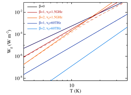
Figure 3: Power radiated by an optically thin greybody vs temperature, for different choices of $\beta$ and $\nu_{0}$. The black solid line corresponds to the blackbody case ($\beta=0$), while red solid lines correspond to $\nu_{0}=1.5$ GHz (i.e. $\lambda_{0}=200~{}\mu$m; dark red: $\beta=1$; light red: $\beta=2$) and blue solid lines correspond to $\nu_{0}=60$ THz (i.e. $\lambda_{0}=5~{}\mu$m; dark blue: $\beta=1$; light blue: $\beta=2$). Dashed lines represent the optically thick greybody (Equation 1): the same color corresponds to the same parameter combination reported above. Note that for $\nu_{0}=60$ THz the two regimes turn out to be indistinguishable in the temperature range shown here, so that dashed lines are completely superposed on the solid lines, then invisible The point where the power of the greybody intersects the power of the blackbody marks the temperature above which the condition of optically thin medium is violated and Equation 31 is no longer valid.

In Figure 3 the $W_{\mathrm{g}}$ vs $T$ relation is displayed for some choices of the parameters $\beta$ (including the blackbody case) and $\nu_{0}$. Also in this case it is possible to notice that the blackbody is the best radiator at the probed temperatures, but all lines with $\beta>0$ appear steeper than the blackbody one, therefore there is an intersection point at some $T_{\mathrm{int}}$ such that a given line is higher than the blackbody one at $T>T_{\mathrm{int}}$. This situation is unphysical because no thermal spectrum can radiate more than the blackbody at the same temperature. This means that above $T_{\mathrm{int}}$ the hypothesis of optically thin medium is violated and to use Equation 6, or 8, is not justified.

Combining Equations 25 and 31 one finds

$$T_{\mathrm{int}}=\frac{h\,\nu_{0}}{k_{B}}\,\left(\frac{h^{3}\,c^{2}}{2\,\pi\,\sigma\,k_{B}^{4}\,\zeta(4+\beta)\,\Gamma(4+\beta)}\right)^{\frac{1}{\beta}}\,.$$ (32)

The above relation indicates that, if $\nu_{0}$ decreases (i.e. the greybody gets optically thin over a shorter range of frequencies), $T_{\mathrm{int}}$ decreases linearly as well, shortening the range of temperatures $T<T_{\mathrm{int}}$ over which $W_{\mathrm{b}}(T)>W_{\mathrm{g}}(T)$, i.e. the physically meaningful case.

This issue is originated by the fact that the integral that leads to Equation (31) is computed over all the frequencies, also those such that $\nu>\nu_{0}$, violating the optically thin assumption. Therefore this equation is still correct only if $\nu_{0}\gg\nu_{*}$, where $\nu_{*}$ is the frequency such that

$$\int_{0}^{\infty}\frac{x^{3+\beta}}{\mathrm{e}^{x}-1}\mathrm{d}x\approx\int_{0}^{x_{*}}\frac{x^{3+\beta}}{\mathrm{e}^{x}-1}\mathrm{d}x\,$$ (33)

where $x_{*}\equiv h\,\nu_{*}/k_{B}\,T$.

We postpone the discussion of this issue to Section 4.2.1, after having approached in Section 4.2 the class of integrals like the one at the right hand side of the above equation.

Finally, we numerically calculated the $W_{\mathrm{g}}(T)$ curves in the optically thick case (for which it is not possible to obtain an analytic relation), and show them in Figure 3. Such curves $i$) do not show a power-law behavior as in the optically thin case; $ii$) do not suffer of the issue of getting higher than the blackbody, being Equation 1 valid at all frequencies; $iii$) are always smaller than the corresponding optically thin case; $iv$) at increasing $\nu_{0}$ and for opportunely low values of $T$ (as those probed in the figure), the optically thick and thin cases get practically indistinguishable (since the Equation 6 is valid over most of the frequency range).

4.1 The $L_{\mathrm{bol}}/M$ ratio

The ratio between the bolometric luminosity of a core/clump, due to the contribution of a possible contained young stellar object and by the residual matter in the parental core/clump, and its mass $M$ is a largely used tool for characterizing the star formation ongoing in a such structure (Molinari et al., 2008; Elia et al., 2013). Indeed, an increase of $L_{\mathrm{bol}}$ is expected as the central source evolves and its temperature increases (so the emission peak shifts towards shorter wavelengths); this is evident especialy during the main accretion phase (Molinari et al., 2008, and references therein). Dividing $L_{\mathrm{bol}}$ by the total envelope mass removes any dependence on the total amount of emitting matter. Interestingly, a $L_{\mathrm{bol}}/M$ built in this way is also a distance-independent quantity. It is important to show the relation between $L_{\mathrm{bol}}/M$ and $T$ for an optically thin greybody, which corresponds to the case of a starless core/clump, to evaluate departures from this behavior, typical of proto-stellar source.

On one hand, the bolometric luminosity of a greybody located at a distance $d$ is observationally evaluated starting from the measured flux:

$$L_{\mathrm{bol}}=4\,\pi\,d^{2}\int_{0}^{\infty}F_{\nu}\,\mathrm{d}\nu\,.$$ (34)

On the other hand, $L_{\mathrm{bol}}=W_{\mathrm{gb}}$, so using Equation 8 for $F_{\nu}$, one obtains

$$\begin{split}&\frac{L_{\mathrm{bol}}}{M}&=&\frac{4\,\pi\,\kappa_{\mathrm{ref}}}{\nu_{\mathrm{ref}}^{\beta}}\int_{0}^{\infty}\nu^{\beta}B_{\nu}(T)\,\mathrm{d}\nu=\\ &&=&4\,\kappa_{\mathrm{ref}}\left(\frac{\nu_{0}}{\nu_{\mathrm{ref}}}\right)^{\beta}\,W_{\mathrm{g}}=\\ &&=&\frac{8\,\pi\,k_{B}^{4+\beta}\,\zeta(4+\beta)\,\Gamma(4+\beta)\,\kappa_{\mathrm{ref}}}{h^{3+\beta}\,c^{2}\,\nu_{\mathrm{ref}}^{\beta}}~{}T^{4+\beta}\,,\end{split}$$ (35)

which is dependent again on $T^{4+\beta}$, but independent on $\nu_{0}$, in the limit of Equation 33.

4.2 The $L_{\mathrm{smm}}/L_{\mathrm{bol}}$ ratio

Another quantity involving the bolometric luminosity and used to characterize the evolutionary state of young stellar objects is the $L_{\mathrm{smm}}/L_{\mathrm{bol}}$ ratio (André et al., 2000), where $L_{\mathrm{smm}}$ is the fraction of $L_{\mathrm{bol}}$ for the sub-millimeter domain, i.e. for $\lambda$ larger than a certain $\lambda_{\mathrm{smm}}$. For example, with respect to the Class 0/I/II/III classification of low-mass young stellar objects (Lada & Wilking, 1984; Lada, 1987; Andre et al., 1993), André et al. (2000) recognized as Class 0 those objects with $L_{\mathrm{smm}}/L_{\mathrm{bol}}>0.005$, for $\lambda_{\mathrm{smm}}=350\mu$m.

For an optically thin greybody, the dependence of this ratio on the greybody parameters can be ascertained starting from Equation 34 as follows :

$$\begin{split}L_{\mathrm{smm}}/L_{\mathrm{bol}}&=&\frac{\int_{0}^{\nu_{\mathrm{smm}}}F_{\nu}\,\mathrm{d}\nu}{\int_{0}^{\infty}F_{\nu}\,\mathrm{d}\nu}=\frac{\int_{0}^{x_{\mathrm{smm}}}\frac{x^{3+\beta}}{\left(\mathrm{e}^{x}-1\right)}\,\mathrm{d}x}{\int_{0}^{\infty}\frac{x^{3+\beta}}{\left(\mathrm{e}^{x}-1\right)}\,\mathrm{d}x}=\\ &=&\frac{\sum_{n=1}^{\infty}\frac{1}{n^{4+\beta}}\int_{0}^{nx_{\mathrm{smm}}}y^{3+\beta}\mathrm{e}^{-y}~{}\mathrm{d}y}{\zeta(4+\beta)\Gamma(4+\beta)}\,,\end{split}$$ (36)

where $\nu_{\mathrm{smm}}=c/\lambda_{\mathrm{smm}}$ is the frequency assumed as the upper end of the sub-mm domain and $x_{\mathrm{smm}}\equiv h\,\nu_{\mathrm{smm}}/k_{B}T$. While the denominator of the last member does not depend on $T$ (see Equation 30), the numerator contains an integral with a finite upper integration limit containing in turn the temperature, which requires a more complex treatment. One needs to invoke the concept of lower incomplete gamma function, defined as $\gamma(s,a)\equiv\int_{0}^{a}y^{s-1}\,\mathrm{e}^{-y}\,dy$. It is found (e.g., Press et al., 2007) that

$$\gamma(s,a)=a^{s}\mathrm{e}^{-a}{s}\,\sum_{i=0}^{\infty}\frac{\Gamma(s)}{\Gamma(s+1+i)}a^{i}\,,$$ (37)

Therefore, being in this case $s=\beta+4$ and $a=n\,x_{\mathrm{smm}}$,

$$\begin{split}&\int_{0}^{nx_{\mathrm{smm}}}y^{3+\beta}\mathrm{e}^{-y}~{}dy=\\ &=\Gamma(4+\beta)(n\,x_{\mathrm{smm}})^{4+\beta}\,\mathrm{e}^{-n\,x_{\mathrm{smm}}}\,\sum_{i=0}^{\infty}\frac{(n\,x_{\mathrm{smm}})^{i}}{\Gamma(5+\beta+i)}\,.\end{split}$$ (38)

So, Equation 36 becomes

$$\begin{split}L_{\mathrm{smm}}/L_{\mathrm{bol}}=\frac{1}{\zeta(4+\beta)}\,\sum_{n=1}^{\infty}\mathrm{e}^{-n\,x_{\mathrm{smm}}}\,\sum_{i=0}^{\infty}\frac{n^{i}}{\Gamma(5+\beta+i)}x_{\mathrm{smm}}^{4+\beta+i}\end{split}$$ (39)

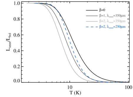
Figure 4: Plot of the $L_{\mathrm{smm}}/L_{\mathrm{bol}}$ ratio vs $T$ relation, as expressed by Equation 39. The grey lines correspond to $\lambda_{\mathrm{smm}}=350~{}\mu$m and different values of $\beta$: 0 (black), 1 (dark grey), and 2 (light grey). The blue dashed line corresponds to the case $\lambda_{\mathrm{smm}}=250~{}\mu$m and $\beta=2$.

In Figure 4 the behavior of $L_{\mathrm{smm}}/L_{\mathrm{bol}}$ vs $T$ is shown for different choices of $\beta$ and $\nu_{\mathrm{smm}}$.

4.2.1 A by-product: discussing Equation 33

Here we exploit the results found for the integration of the greybody over a non-infinite range (i.e., Equation 37) to conclude the discussion about Equation 33, namely regarding the frequency $\nu_{*}$ such that, given $x_{*}=h\,\nu_{1}/k_{B}\,T$, the condition, say, $R\equiv\int_{0}^{x_{*}}\frac{x^{3+\beta}}{\mathrm{e}^{x}-1}\,\mathrm{d}x/\int_{0}^{\infty}\frac{x^{3+\beta}}{\mathrm{e}^{x}-1}\,\mathrm{d}x>99\%$ is satisfied. The ratio $R$ coincides exactly with the case of Equation 36 fully developed through Equation 39, with $\nu_{1}$ playing in this case the role of $\nu_{\mathrm{smm}}$ in those equations.

For a precision of 10% (i.e. $R=0.1$), $x_{*}\geq 8$ when $\beta=1$, and $x_{*}\geq 11$ for $\beta=3$. Turning $x_{*}$ in a wavelength, one finds $\lambda_{*}$($\mu$mm)$=1308/T$(K) and $\lambda_{*}$($\mu$m)$=1798/T$(K), for $\beta=3$ and 1, respectively. For instance, for a SED with $T=20$ K and $\beta=1$, the greybody must be already optically thin at $\lambda_{*}=90~{}\mu$m, while for $T=30$ K the limit on being optically thin is pushed down to $60~{}\mu$m.

Clearly, these values for $\lambda_{*}$ apply to SED known over the infinite range $\lambda_{*}\leq\lambda<\infty$. To be less generic, let us consider the practical case of a SED which is known only at five Herschel bands: the two 70 $\mu$m and 160 $\mu$m for PACS, and the three SPIRE bands 250 $\mu$m, 350 $\mu$m and 500 $\mu$m. This is the case for the Herschel surveys already mentioned: GBS, HOBYS, and HIGAL. We derived the theoretical SEDs from Equation 1 for $\lambda_{0}=10$, 50, and 100 $\mu$m, and for $\beta=1$,2 and 3; for the temperature we explored the range $5\leq T\leq 50$ K in steps of 1 K.

For each SED we computed the true luminosity ($L_{\mathrm{thick}}$) by numerical integration of Equation 1 from $1~{}\mu$m to 1 mm: in the upper panel of Figure 5 we show the ratio between $L_{\mathrm{thick}}$ and the luminosity $L_{\mathrm{H}}$ computed integrating the five-band Herschel SED. This figure shows the error associated to a Herschel-derived luminosity. However, this is only of mathematical interest because in the most common case the astronomer does not know $\beta$, so that it is not known with which curve $L_{\mathrm{H}}$ should be compared.

The other two panels are more interesting because we compared the true luminosity with two quantities derivable from the data. Since we are assuming that only the five Herschel fluxes are known (we used five bands, but including the 100 $\mu$m PACS band too would not alter our conclusions), it is not possible to derive a robust estimate of $\beta$ directly from the observed values, so that we fix $\beta=2$, a common choice when dealing only with Herschel data (Sadavoy et al., 2013). For any theoretical SED, we looked for the best-fitting optically thin greybody with $\beta=2$. For this greybody, we computed both the luminosity $L_{\mathrm{H2}}$ obtained integrating only the fluxes at the five considered wavelengths, and the luminosity $L_{\mathrm{an2}}$ given by Equation 31. The ratios between these two luminosities and the true luminosity $L_{\mathrm{thick}}$ are shown in the central and bottom panels of Figure 5, respectively. For simplicity, the $x$-axis reports the true temperature in both cases, although the temperature used to compute the luminosity is that derived from the fit. The central panel of Figure 5 is, qualitatively, quite similar to the top panel and shows an erratic behaviour of the ratio: the agreement is within 20% (limit shown by means of the two black horizontal lines) for $T\ga 10$ K, but the upper limit on $T$, where the agreement is good, strongly depends on $\beta$, which is unknown. The bottom panel, on the contrary, shows a ratio contained in the 20% limits for all the $T\ga 10$ K up to 50 K, the highest $T$ used in the synthetic SEDs. Only for $\beta$ as high as 3 there are ranges of $T$ for which the agreement is not good.

Our conclusion is that once an astronomer decides to fit an observed SED with an optically thin greybody with $\beta=2$, it is better to compute the luminosity from Equation 31 rather than to integrate the observed fluxes, or those derived from the fit. The case in which $\beta$ is known from the data is dealt with in Section 6.

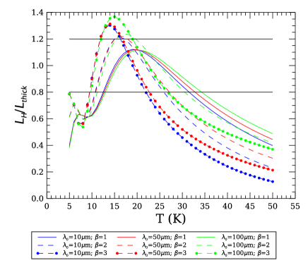
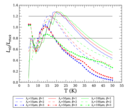
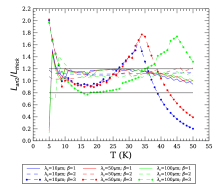
Figure 5: Ratios between three different estimates of the luminosity of a SED and $L_{\mathrm{thick}}$, i.e. the luminosity of a greybody obtained by numerical integration of Equation 1 (considered here as the true luminosity of the SED), vs greybody temperature. Top: ratio between $L_{\mathrm{H}}$, obtained by integrating the SED observed by Herschel, and $L_{\mathrm{thick}}$. Centre: ratio between $L_{\mathrm{H2}}$, obtained by numerical integration of an optically-thin model with $\beta=2$, best-fitting the SED observed by Herschel, and $L_{\mathrm{thick}}$. Bottom: ratio between $L_{\mathrm{an2}}$, obtained directly through Equation 31 with $\beta=2$ and $T$ derived by the same fit as in the previous panel, and $L_{\mathrm{thick}}$. The horizontal black lines show the 20% agreement zone.

5 Bolometric temperature

The bolometric temperature $T_{\mathrm{bol}}$ (Myers & Ladd, 1993) is another quantity used in the study of star formation to quantify the evolutionary status of young stellar objects. Indeed it constitutes an estimate, in units of temperature, of the “average frequency” of a SED (with the fluxes composing the SED used as weights):

$$\bar{\nu}=\frac{\int_{0}^{\infty}\nu\,I_{\nu}~{}\mathrm{d}\nu}{\int_{0}^{\infty}~{}I_{\nu}~{}\mathrm{d}\nu}\,.$$ (40)

For a blackbody, exploiting Equation 31, one finds

$$\bar{\nu}_{\mathrm{bb}}=\frac{\int_{0}^{\infty}\nu\,B_{\nu}(T)~{}\mathrm{d}\nu}{\int_{0}^{\infty}~{}B_{\nu}(T)~{}\mathrm{d}\nu}=\frac{4\,k_{B}}{h}\frac{\zeta(5)}{\zeta(4)}\,T\,.$$ (41)

Rigorously, the bolometric temperature of a generic source is defined as the temperature of a blackbody having the same mean frequency $\bar{\nu}$:

$$T_{\mathrm{bol}}=\frac{h}{4\,k_{B}}\,\frac{\zeta(4)}{\zeta(5)}\bar{\nu}=\frac{h}{4\,k_{B}}\,\frac{\zeta(4)}{\zeta(5)}\,\frac{\int_{0}^{\infty}\nu\,F_{\nu}~{}\mathrm{d}\nu}{\int_{0}^{\infty}~{}F_{\nu}~{}\mathrm{d}\nu}\,.$$ (42)

In this definition, (Myers & Ladd, 1993) adopted a normalization suggested by Equation 41 to obtain $T_{\mathrm{bol}}=T$ for the blackbody case.

Looking at different phases of star formation, the transition from Class 0 to Class I and then to Class II sources is characterized by a temperature getting warmer and warmer and the SED getting brighter and brighter in the near- and mid-infrared: as a consequence of this, also $\bar{\nu}$ and $T_{\mathrm{bol}}$ increase. In this respect, Chen et al. (1995), suggested to identify the aforementioned evolutionary classes through $T_{\mathrm{bol}}$.

Here we explore the analytic behavior of the bolometric temperature of an optically thin greybody as a function of the various involved parameters. Combining Equations 41, 8, and 31, one obtains

$$\begin{split}\nu_{\mathrm{gb}}&=\frac{\int_{0}^{\infty}\nu^{1+\beta}~{}B_{\nu}(T)~{}\mathrm{d}\nu}{\int_{0}^{\infty}~{}\nu^{\beta}~{}B_{\nu}(T)~{}\mathrm{d}\nu}=&\\ &=\frac{k_{B}\zeta(5+\beta)\Gamma(5+\beta)}{h\,\zeta(4+\beta)\Gamma(4+\beta)}\,T=&\\ &=\frac{k_{B}}{h}\frac{\zeta(5+\beta)}{\zeta(4+\beta)}\,T\,,&\end{split}$$ (43)

so that the bolometric temperature for a greybody is given by

$$T_{\mathrm{bol}}=\frac{4+\beta}{4}\frac{\zeta(4)\zeta(5+\beta)}{\zeta(5)\zeta(4+\beta)}\,T\,.$$ (44)

It is noteworthy that in this relation the proportionality factor between $T_{\mathrm{bol}}$ and $T$ is a monotonically increasing function of $\beta$ being in turn the product of two increasing functions, as illustrated in Figure 6.

Figure 6: Solid line: behavior of the multiplicative term in front of $T$ in the expression of $T_{\mathrm{bol}}$ (Equation 44), namely $[(4+\beta)\zeta(4)\zeta(5+\beta)]/[4\,\zeta(5)\zeta(4+\beta)]$, as a function of $\beta$. Dashed line: behavior of $\zeta(5+\beta)/\zeta(4+\beta)$ as a function of $\beta$.

Furthermore, since $\zeta(4)/\zeta(5)\simeq 1.044$, for $\beta=1$ the ratio of the $\zeta$ functions differ from 1 by $\sim$2%, and by $\sim$1% for $\beta=2$. One makes then a very small error putting $\zeta(5+\beta)/\zeta(4+\beta)=1$, so that

$$T_{\mathrm{bol}}=\frac{4+\beta}{4}\,T~{}\,\,(\mathrm{for\ }\beta\geq 1)\,.$$ (45)

As an immediate consequence, a greybody source with $\beta=2$ and $T>47$ K has $T_{\mathrm{bol}}>70$ K, i.e. above the boundary between Class 0 and Class I established by Chen et al. (1995).

6 An alternative way to estimate $T$ and $\beta$ for an observed SED

Equation 43 represents the the first moment of the distribution of an optically thin greybody, hereafter $\nu_{1}$. In general, the $n$-th moment can be straightforwardly calculated as:

$$\nu_{n}=\left(\frac{k_{B}\,T}{h}\right)^{n}\frac{\Gamma(n+4+\beta)\zeta(n+4+\beta)}{\Gamma(4+\beta)\zeta(4+\beta)}\,.$$ (46)

So, computing now the second moment one finds

$$\begin{split}\nu_{2}&=\left(\frac{k_{B}\,T}{h}\right)^{2}\frac{\Gamma(6+\beta)\zeta(6+\beta)}{\Gamma(4+\beta)\zeta(4+\beta)}\,.\end{split}$$ (47)

As shown above, one can put $\zeta(6+\beta)/\zeta(4+\beta)\sim 1$ so that

$$\nu_{2}=(5+\beta)(4+\beta)\left(\frac{k_{B}\,T}{h}\right)^{2}\,\,\,\,\,(\mathrm{for\ }\beta\geq 1)\,.$$ (48)

Combining Equations 43 and 48, one finds the interesting relation

$$\beta=\frac{5\nu_{1}^{2}-4\nu_{2}}{\nu_{2}-\nu_{1}^{2}}\,.$$ (49)

In the same way, by a combination of these two frequencies (actually $\nu_{2}$ has the unit of Hz²) it is possible to derive the formula for the temperature

$$T=\frac{h}{k_{B}}\left(\frac{\nu_{2}}{\nu_{1}}-\nu_{1}\right)\,.$$ (50)

These two equations give the exact values of $\beta$ and $T$, provided that the spectrum is known over a wide range of frequencies (or wavelengths). In reality this is not always true: the smaller the number of data points, the higher the error associated with these equations.

To give an idea of the applicability of these two formulae, we took from literature the case of the the candidate first-hydrostatic core CB17MMS (Chen et al., 2012): the authors report the fluxes at 100 $\mu$m, 160 $\mu$m, 850 $\mu$m and 1.3 mm, so just four wavelengths. From these data we computed, with a straightforward application of the trapezium rule, $\nu_{1}$ and $\nu_{2}$. As a second step, we generated a grid of models, with $5\leq T(\mathrm{K})\leq 50$ and $1\leq\beta\leq 3$, at the same four aforementioned wavelengths. For each model we computed the expected values $\bar{\nu_{1}}$ and $\bar{\nu_{2}}$, that are compared with the values derived from the observations $\nu_{1}$ and $\nu_{2}$: we looked for the minimum of the residuals defined as

$$\delta\equiv\left(\frac{(\bar{\nu_{1}}-\nu_{1})}{\mathrm{max}(\bar{\nu_{1}})}\right)^{2}+\left(\frac{(\bar{\nu_{2}}-\nu_{2})}{\mathrm{max}(\bar{\nu_{2}})}\right)^{2}\,,$$ (51)

where the normalization is necessary due to the fact that, for the same model, $\bar{\nu_{2}}$ is of the order of $\bar{\nu_{1}}^{2}$: indeed, without this normalization, $\delta$ would be dominated by the term containing $\nu_{1}$. All the models in the grid, constructed in steps of $0.1$ K in $T$ and $0.1$ in $\beta$, were sorted by increasing residuals. The best model, corresponding to the lowest $\delta$, provides $T$ and $\beta$, whereas the ten best models are taken into account to evaluate the spread of these two parameters, hence the uncertainty affecting them. The final result is $T=10.6\pm 1.3$ K and $\beta=2.1\pm 0.6$. These values are in good agreement with those reported by Chen et al. (2012), namely $T\sim 10$ K and $\beta=1.8$. Notice that if we would have just used $\nu_{1}$ and $\nu_{2}$ to derive directly $T$ and $\beta$, the result would have been $T=7.8$ K and $\beta=6.5$, which is unphysical.

Now, if we measure the luminosity of the object, again through the trapezium rule, we find $L=0.18~{}L_{\odot}$, at the distance of 250 pc. This luminosity can be compared with that expected theoretically (Equation 31) which depends on $T$, $\beta$, the solid angle and $\nu_{0}$; unfortunately Chen et al. (2012) did not provide the solid angle in their paper, but the fluxes they reported for CB17MMS were derived with apertures ranging from 10″to 20″: estimating the solid angle from these apertures, Equation 31 tells us that the wavelength at wich $\tau=1$ is in the range $30\lesssim\lambda_{0}(\mu\mathrm{m})\lesssim 58$, which looks reasonable.

As another example we consider the SED of GG Tau A as reported by Scaife (2013): in this case the SED is emitted by a disc so that the hypothesis of a single-temperature optically-thin greybody is very coarse, but still our results can be compared with those of the author. Our procedure, applied to the SED from 100 $\mu$m to 1.86 cm, gives $T=18.5\pm 6.7$ K and $\beta=1.1\pm 1.7$. Our $T$ agrees well with the reported value of $T=19.42\pm 0.55$ K; the value of $\beta$ has a large uncertainty but the best-fit value, $\beta=1.1$, is also in agreement with the value of Scaife (2013), $0.96\pm 0.04$. Since $T(R=300\mathrm{AU})\approx 20$ K, as reported by the author, we took this radius as an estimate of the solid angle, given the distance of 140 pc, and we found $\lambda_{0}\sim 29$ $\mu$m.

As a last example, we used the compilation of fluxes reported recently by Ren & Li (2016) for a set of sources in NGC 2024 whose SEDs are built from 70 to 850 $\mu$m. In Table 2 we reported the name of each source, $T$, $\beta$ and $L_{\mathrm{bol}}$ as computed by the authors, the same quantities as computed by us, and, in the last column, $\lambda_{0}$.

The source FIR-1 gives a result compatible with the hypothesis of an optically thin greybody ($\lambda_{0}<\lambda_{\mathrm{min}}$) only if set $\lambda_{\mathrm{min}}=160$ $\mu$m, i.e., after discarding the first two available wavelengths; the same happens with FIR-2 and FIR-3 as well. For FIR-4 and FIR-6 the whole SED has been used, as the resulting $\lambda_{0}$ is smaller than 70 $\mu$m. FIR-5 is resolved in two sources at 450 $\mu$m and not resolved at the other wavelengths: for this reason we decided not to consider this source. Finally, the SED of FIR-7 has been limited to $\lambda\geq 250~{}\mu$m to fulfill the condition $\lambda_{0}<\lambda_{\mathrm{min}}$.

Clearly, our $L_{\mathrm{bol}}$ are smaller than values of Ren & Li (2016) because they were evaluated over a shorter range of wavelengths: if we trust the values of $\lambda_{0}$ found, our luminosities constitute an estimate of the optically-thin contribution to $L_{\mathrm{bol}}$ for each source. The large uncertainty in $T$ for FIR-7 clearly reflects the fact that we derived the physical parameters of this source at large wavelengths, excluding the peak of the SED.

In the examples reported above we have shown in a number of cases how well, or how bad, our Equations 46 and 47 can be used to extract physical informations from a SED: one may wonder why Equations 49 and 50 should be used to find $\beta$ and $T$ instead of using well-known routines that can solve the non-linear least-squares problems. There are a few advantages, indeed: first, one does not need to give initial values for the parameters, which not always are obvious to be estimated. Second, specifically to the greybody problem, it is often assumed that, for Herschel data, it is not possible to have realistic estimates of both $\beta$ and $T$, given the well-known degeneracy between these two values (Juvela et al., 2013), as it can be seen in Equation 12. On the contrary, our formulae do not imply a fitting procedure, and give the two parameters without being affected by degeneracy. Third, if the distance and the solid angle are known for a source, one can derive also $\lambda_{0}$, i.e. the wavelength at which $\tau=1$. In the usual formalism given by, e.g., Equation 8, there is no way to derive $\lambda_{0}$ from the data. As a consequence of this, with our method the astronomer can judge a posteriori if the derived values are consistent with the optically-thin hypothesis, something that seldom is done in literature.

Of course, we should not forget that inferring $T$ and $\beta$ from real observations is more challenging because of line of sight mixing of temperature (breaking the condition of isothermal emission), asymmetric illumination of target source, and contribution of different population of dust grains to the net emission. But these caveats affect any kind of fitting procedure.

Table 2: Results of applying Equations 49 and 50 to source SEDs of Ren & Li (2016)^a.

	Ren & Li (2016)				This paper
Name	$T$	$\beta$	$L_{\mathrm{bol}}$		$T$	$\beta$	$L_{\mathrm{bol}}$	$\lambda_{0}$
	K		$L_{\odot}$		K		$L_{\odot}$	$\mu$m
FIR-1	18.5	2.5	80		$29.3\pm 8.7$	$1.6\pm 0.4$	22	19
FIR-2	18.0	2.7	130		$18.4\pm 4.3$	$2.4\pm 0.6$	32	145
FIR-3	17.5	2.6	220		$19.0\pm 3.4$	$2.3\pm 0.7$	47	141
FIR-4	22.0	2.9	570		$32.2\pm 3.1$	$1.3\pm 0.3$	221	64
FIR-6	18.5	2.7	160		$26.1\pm 2.4$	$1.0\pm 0.4$	118	43
FIR-7	18.0	2.6	110		$19\pm 12$	$2.8\pm 0.7$	8	70
a We used the whole SED, from 70 $\mu$m to 850 $\mu$m, for FIR-4 and 6;
from 160 $\mu$m to 850 $\mu$m for FIR-1, FIR-2, and FIR-3;
from 250 $\mu$m to 850 $\mu$m for FIR-7.

Finally, we provide an example of application of Equation 41 to derive $T$ for a blackbody from an observed SED. We consider the COBE-FIRAS spectrum of the cosmic microwave background radiation measured by Fixsen et al. (1996). The temperature derived through Equation 41 is 2.82 K, only 3% higher than the 2.725 K value used by the authors to derive the monopole spectrum.

7 Conclusions

In this paper we collected and re-arranged a number of dispersed analytic relations among the parameters of a greybody, developing further equations and discussing the errors involved by typical approximations. This is certainly of some interest for astronomers who model the Galactic and extragalactic cold dust emission as a greybody, especially in the current “Herschel era”, characterized by the availability of huge archives of photometric far-infrared data. In particular,

• The position of the peak of the greybody emission, in terms of both frequency and wavelength as a function of the temperature has been revised, considering deviations from the classical blackbody. Approximated expressions for it are suggested in correspondence of different regimes of optical thickness.

• Quantities typically exploited in the study of early phases of star formation have been discussed in the case of an optically thin greybody. The bolometric luminosity of a greybody shows a power-law dependence on the temperature, with exponent $4+\beta$, representing a general case of which the Stefan-Boltzmann’s law is a particular case for $\beta=0$ (blackbody).

• The ratio between the so-called sub-millimeter luminosity and the bolometric one, which is used to recognize Class 0 young stellar objects, shows a more complex behavior. The temperature at which this ratio gets larger than 0.05% (so early-phase star forming cores/clumps are identified) decreases at increasing $\beta$.

• The bolometric temperature of a greybody is found to be linearly related to the temperature, through a multiplicative constant that depends only on $\beta$ and can be further simplified for $\beta\geq 1$.

• We indicate a method to derive the temperature and the dust emissivity law exponent of a greybody, or simply the temperature of a blackbody, modeling an observed SED without performing a best-fit procedure. We report and discuss the conditions for the applicability of this method, which appears well suitable for well-sampled SEDs and in the range of temperatures typical of cold dense cores/clumps.

References

- Andre et al. (1993) Andre P., Ward-Thompson D., Barsony M., 1993, ApJ, 406, 122
- André et al. (2000) André P., Ward-Thompson D., Barsony M., 2000, Protostars and Planets IV, p. 59
- André et al. (2010) André P., et al., 2010, A&A, 518, L102
- Chen et al. (1995) Chen H., Myers P. C., Ladd E. F., Wood D. O. S., 1995, ApJ, 445, 377
- Chen et al. (2012) Chen X., Arce H. G., Dunham M. M., Zhang Q., Bourke T. L., Launhardt R., Schmalzl M., Henning T., 2012, ApJ, 751, 89
- Choudhuri (2010) Choudhuri A. R., 2010, Astrophysics for Physicists
- Elia et al. (2010) Elia D., et al., 2010, A&A, 518, L97
- Elia et al. (2013) Elia D., et al., 2013, ApJ, 772, 45
- Faúndez et al. (2004) Faúndez S., Bronfman L., Garay G., Chini R., Nyman L.-Å., May J., 2004, A&A, 426, 97
- Fixsen et al. (1996) Fixsen D. J., Cheng E. S., Gales J. M., Mather J. C., Shafer R. A., Wright E. L., 1996, ApJ, 473, 576
- Giannini et al. (2012) Giannini T., et al., 2012, A&A, 539, A156
- Gordon (1995) Gordon M. A., 1995, A&A, 301, 853
- Hildebrand (1983) Hildebrand R. H., 1983, QJRAS, 24, 267
- Juvela et al. (2013) Juvela M., Montillaud J., Ysard N., Lunttila T., 2013, A&A, 556, A63
- Könyves et al. (2010) Könyves V., et al., 2010, A&A, 518, L106
- Lada (1987) Lada C. J., 1987, in Peimbert M., Jugaku J., eds, IAU Symposium Vol. 115, Star Forming Regions. pp 1–17
- Lada & Wilking (1984) Lada C. J., Wilking B. A., 1984, ApJ, 287, 610
- Molinari et al. (2008) Molinari S., Pezzuto S., Cesaroni R., Brand J., Faustini F., Testi L., 2008, A&A, 481, 345
- Molinari et al. (2010) Molinari S., et al., 2010, PASP, 122, 314
- Mookerjea et al. (2007) Mookerjea B., Sandell G., Stutzki J., Wouterloot J. G. A., 2007, A&A, 473, 485
- Motte et al. (2010) Motte F., et al., 2010, A&A, 518, L77
- Myers & Ladd (1993) Myers P. C., Ladd E. F., 1993, ApJ, 413, L47
- Myers et al. (1998) Myers P. C., Adams F. C., Chen H., Schaff E., 1998, ApJ, 492, 703
- Olmi et al. (2009) Olmi L., et al., 2009, ApJ, 707, 1836
- Pezzuto et al. (2012) Pezzuto S., et al., 2012, A&A, 547, A54
- Pilbratt et al. (2010) Pilbratt G. L., et al., 2010, A&A, 518, L1
- Press et al. (2007) Press W. H., Teukolsky S. A., Vetterling W. T., Flannery B. P., 2007, Numerical Recipes 3rd Edition: The Art of Scientific Computing, 3 edn. Cambridge University Press, New York, NY, USA
- Ragan et al. (2012) Ragan S., et al., 2012, A&A, 547, A49
- Ren & Li (2016) Ren Z., Li D., 2016, preprint, (arXiv:1604.08415)
- Rybicki & Lightman (1979) Rybicki G. B., Lightman A. P., 1979, Radiative processes in astrophysics
- Sadavoy et al. (2013) Sadavoy S. I., et al., 2013, ApJ, 767, 126
- Scaife (2013) Scaife A. M. M., 2013, MNRAS, 435, 1139
- Strafella et al. (2015) Strafella F., et al., 2015, ApJ, 798, 104