Multiple-Play Bandits in the Position-Based Model

Abstract

Sequentially learning to place items in multi-position displays or lists is a task that can be cast into the multiple-play semi-bandit setting. However, a major concern in this context is when the system cannot decide whether the user feedback for each item is actually exploitable. Indeed, much of the content may have been simply ignored by the user. The present work proposes to exploit available information regarding the display position bias under the so-called Position-based click model (PBM). We first discuss how this model differs from the Cascade model and its variants considered in several recent works on multiple-play bandits. We then provide a novel regret lower bound for this model as well as computationally efficient algorithms that display good empirical and theoretical performance.

1 Introduction

During their browsing experience, users are constantly provided – without having asked for it – with clickable content spread over web pages. While users interact on a website, they send clicks to the system for a very limited selection of the clickable content. Hence, they let every unclicked item with an equivocal answer: the system does not know whether the content was really deemed irrelevant or simply ignored. In contrast, in traditional multi-armed bandit (MAB) models, the learner makes actions and observes at each round the reward corresponding to the chosen action. In the so-called multiple play semi-bandit setting, when users are presented with $L$ items, they are assumed to provide feedback for each of those items.

Several variants of this basic setting have been considered in the bandit literature. The necessity for the user to provide feedback for each item has been called into question in the context of the so-called Cascade Model [7, 13, 5] and its extensions such as the Dependent Click Model (DCM) [19]. Both models are particularly suited for search contexts, where the user is assumed to be looking for something relative to a query. Consequently, the learner expects explicit feedback: in the Cascade Model each valid observation sequence must be either all zeros or terminated by a one, such that no ambiguity is left on the evaluation of the presented items, while multiple clicks are allowed in the DCM.

In the Cascade Model, the positions of the items are not taken into account in the reward process because the learner is assumed to obtain a click as long as the interesting item belongs to the list. Indeed, there are even clear indications that the optimal strategy in a learning context consists in showing the most relevant items at the end of the list in order to maximize the amount of observed feedback [13] – which is counter-intuitive in recommendation tasks.

To overcome these limitations, [5] introduces weights – to be defined by the learner – that are attributed to positions in the list, with a click on position $l\in\{1,\dots,L\}$ providing a reward $w_{l}$, where the sequence $(w_{l})_{l}$ is decreasing to enforce the ranking behavior. However, no rule is given for setting the weights $(w_{l})_{l}$ that control the order of importance of the positions. The authors propose an algorithm based on KL-UCB [9] and prove a lower bound on the regret as well as an asymptotically optimal upper bound.

Another way to address the limitations of the Cascade Model is to consider the DCM as in [19]. Here, examination probabilities $v_{l}$ are introduced for each position $l$: conditionally on the event that the user effectively scanned the list up to position $l$, he/she can choose to leave with probability $v_{l}$ and in that case, the learner is aware of his/her departure. This framework naturally induces the necessity to rank the items in the optimal order.

All previous models assume that a portion of the recommendation list is explicitly examined by the user and hence that the learning algorithm eventually has access to rewards corresponding to the unbiased user’s evaluation of each item. In contrast, we propose to analyze multiple-play bandits in the Position-based model (PBM) [4]. In the PBM, each position in the list is also endowed with a binary Examination variable [7, 18] which is equal to one only when the user paid attention to the corresponding item. But this variable, that is independent of the user’s evaluation of the item, is not observable. It allows to model situations where the user is not explicitly looking for specific content, as in typical recommendation scenarios.

Compared to variants of the Cascade model, the PBM is challenging due to the censoring induced by the examination variables: the learning algorithm observes actual clicks but non-clicks are always ambiguous. Thus, combining observations made at different positions becomes a non-trivial statistical task. Some preliminary ideas on how to address this issue appear in the supplementary material of [12]. In this work, we provide a complete statistical study of stochastic multiple-play bandits with semi-bandit feedback in the PBM.

We introduce the model and notations in Section 2 and provide the lower bound on the regret in Section 3. In Section 4, we present two optimistic algorithms as well as a theoretical analysis of their regret. In the last section dedicated to experiments, those policies are compared to several benchmarks on both synthetic and realistic data.

2 Setting and Parameter Estimation

We consider the binary stochastic bandit model with $K$ Bernoulli-distributed arms. The model parameters are the arm expectations $\theta=(\theta_{1},\theta_{2},\ldots,\theta_{K})$, which lie in $\Theta=(0,1)^{K}$. We will denote by $\mathcal{B}(\theta)$ the Bernoulli distribution with parameter $\theta$ and by $d(p,q):=p\log(p/q)+(1-p)\log((1-p)/(1-q))$ the Kullback-Leibler divergence from $\mathcal{B}(p)$ to $\mathcal{B}(q)$. At each round $t$, the learner selects a list of $L$ arms – referred to as an action – chosen among the $K$ arms which are indexed by $k\in\{1,\dots,K\}$. The set of actions is denoted by $\mathcal{A}$ and thus contains $K!/(K-L)!$ ordered lists; the action selected at time $t$ will be denoted $A(t)=(A_{1}(t),\dots,A_{L}(t))$.

The PBM is characterized by examination parameters $(\kappa_{l})_{1\leq l\leq L}$, where $\kappa_{l}$ is the probability that the user effectively observes the item in position $l$ [4]. At round $t$, the selection $A(t)$ is shown to the user and the learner observes the complete feedback – as in semi-bandit models – but the observation at position $l$, $Z_{l}(t)$, is censored being the product of two independent Bernoulli variables $Y_{l}(t)$ and $X_{l}(t)$, where $Y_{l}(t)\sim\mathcal{B}(\kappa_{l})$ is non null when the user considered the item in position $l$ – which is unknown to the learner – and $X_{l}(t)\sim\mathcal{B}(\theta_{A_{l}(t)})$ represents the actual user feedback to the item shown in position $l$. The learner receives a reward $r_{A(t)}=\sum_{l=1}^{L}Z_{l}(t)$, where $Z(t)=(X_{1}(t)Y_{1}(t),\ldots,X_{L}(t)Y_{L}(t))$ denotes the vector of censored observations at step $t$.

In the following, we will assume, without loss of generality, that $\theta_{1}>\dots>\theta_{K}$ and $\kappa_{1}>\dots>\kappa_{L}>0$, in order to simplify the notations. The fact that the sequences $(\theta_{l})_{l}$ and $(\kappa_{l})_{l}$ are decreasing implies that the optimal list is $a^{*}=(1,\ldots,L)$. Denoting by $R(T)=\sum_{t=1}^{T}r_{a^{*}}-r_{A(t)}$ the regret incurred by the learner up to time $T$, one has

$$\mathds{E}[R(T)]=\sum_{t=1}^{T}\sum_{l=1}^{L}\kappa_{l}(\theta_{a^{*}_{l}}-\mathds{E}[\theta_{A_{l}(t)}])=\sum_{a\in\mathcal{A}}\left(\mu^{*}-\mu_{a}\right)\mathds{E}[N_{a}(T)]=\sum_{a\in\mathcal{A}}\Delta_{a}\mathds{E}[N_{a}(T)],$$ (1)

where $\mu_{a}=\sum_{l=1}^{L}\kappa_{l}\theta_{a_{l}}$ is the expected reward of action $a$, $\mu^{*}=\mu_{a^{*}}$ is the best possible reward in average, $\Delta_{a}=\mu^{*}-\mu_{a}$ the expected gap to optimality, and, $N_{a}(T)=\sum_{t=1}^{T}\mathds{1}\{A(t)=a\}$ is the number of times action $a$ has been chosen up to time $T$.

In the following, we assume that the examination parameters $(\kappa_{l})_{1\leq l\leq L}$ are known to the learner. These can be estimated from historical data [4], using, for instance, the EM algorithm [8] (see also Section 5). In most scenarios, it is realistic to assume that the content (e.g., ads in on-line advertising) is changing much more frequently than the layout (web page design for instance) making it possible to have a good knowledge of the click-through biases associated with the display positions.

The main statistical challenge associated with the PBM is that one needs to obtain estimates and confidence bounds for the components $\theta_{k}$ of $\theta$ from the available $\mathcal{B}(\kappa_{l}\theta_{k})$-distributed draws corresponding to occurrences of arm $k$ at various positions $l=1,\dots,L$ in the list. To this aim, we define the following statistics: $S_{k,l}(t)=\sum_{s=1}^{t-1}Z_{l}(s)\mathds{1}\{A_{l}(s)=k\}$, $S_{k}(t)=\sum_{l=1}^{L}S_{k,l}(t)$, $N_{k,l}(t)=\sum_{s=1}^{t-1}\mathds{1}\{A_{l}(s)=k\}$, $N_{k}(t)=\sum_{l=1}^{L}N_{k,l}(t)$. We further require bias-corrected versions of the counts $\tilde{N}_{k,l}(t)=\sum_{s=1}^{t-1}\kappa_{l}\mathds{1}\{A_{l}(s)=k\}$ and $\tilde{N}_{k}(t)=\sum_{l=1}^{L}\tilde{N}_{k,l}(t)$.

A time $t$, and conditionally on the past actions $A(1)$ up to $A(t-1)$, the Fisher information for $\theta_{k}$ is given by $I(\theta_{k})=\sum_{l=1}^{L}N_{k,l}(t)\kappa_{l}/(\theta_{k}(1-\kappa_{l}\theta_{k}))$ (see Appendix A). We cannot however estimate $\theta_{k}$ using the maximum likelihood estimator since it has no closed form expression. Interestingly though, the simple pooled linear estimator

$$\hat{\theta}_{k}(t)=S_{k}(t)/\tilde{N}_{k}(t),$$ (2)

considered in the supplementary material to [12], is unbiased and has a (conditional) variance of $\upsilon(\theta_{k})=(\sum_{l=1}^{L}N_{k,l}(t)\kappa_{l}\theta_{k}(1-\kappa_{l}\theta_{k}))/(\sum_{l=1}^{L}N_{k,l}(t)\kappa_{l})^{2}$, which is close to optimal given the Cramér-Rao lower bound. Indeed, $\upsilon(\theta_{k})I(\theta_{k})$ is recognized as a ratio of a weighted arithmetic mean to the corresponding weighted harmonic mean, which is known to be larger than one, but is upper bounded by $1/(1-\theta_{k})$, irrespectively of the values of the $\kappa_{l}$’s. Hence, if, for instance, we can assume that all $\theta_{k}$’s are smaller than one half, the loss with respect to the best unbiased estimator is no more than a factor of two for the variance. Note that despite its simplicity, $\hat{\theta}_{k}(t)$ cannot be written as a simple sum of conditionally independent increments divided by the number of terms and will thus require specific concentration results.

It can be checked that when $\theta_{k}$ gets very close to one, $\hat{\theta}_{k}(t)$ is no longer close to optimal. This observation also has a Bayesian counterpart that will be discussed in Section 5. Nevertheless, it is always preferable to the “position-debiased” estimator $(\sum_{l=1}^{L}S_{k,l}(t)/\kappa_{l})/N_{k,l}(t)$ which gets very unreliable as soon as one of the $\kappa_{l}$’s gets very small.

3 Lower Bound on the Regret

In this section, we consider the fundamental asymptotic limits of learning performance for online algorithms under the PBM. These cannot be deduced from earlier general results, such as those of [10, 6], due to the censoring in the feedback associated to each action. We detail a simple and general proof scheme – using the results of [11] – that applies to the PBM, as well as to more general models.

Lower bounds on the regret rely on changes of measure: the question is how much can we mistake the true parameters of the problem for others, when observing successive arms? With this in mind, we will subscript all expectations and probabilities by the parameter value and indicate explicitly that the quantities $\mu_{a},a^{*},\mu^{*},\Delta_{a}$, introduced in Section 2, also depend on the parameter. For ease of notation, we will still assume that $\theta$ is such that $a^{*}(\theta)=(1,\dots,L$).

3.1 Existing results for multiple-play bandit problems

Lower bounds on the regret will be proved for uniformly efficient algorithms, in the sense of [15]:

Definition 1.

An algorithm is said to be uniformly efficient if for any bandit model parameterized by $\theta$ and for all $\alpha\in(0,1]$, its expected regret after $T$ rounds is such that $\mathds{E}_{\theta}R(T)=o(T^{\alpha})$.

For the multiple-play MAB, [1] obtained the following bound

$$\liminf_{T\rightarrow\infty}\frac{\mathds{E}_{\theta}R(T)}{\log(T)}\geq\sum_{k=L+1}^{K}\frac{\theta_{L}-\theta_{k}}{d(\theta_{k},\theta_{L})}.$$ (3)

For the “learning to rank” problem where rewards follow the weighted Cascade Model with decreasing weights $\left(w_{l}\right)_{l=1,\ldots,L}$, [5] derived the following bound

$$\liminf_{T\rightarrow\infty}\frac{\mathds{E}_{\theta}R(T)}{\log T}\geq w_{L}\sum_{k=L+1}^{K}\frac{\theta_{L}-\theta_{k}}{d(\theta_{k},\theta_{L})}.$$

Perhaps surprisingly, this lower bound does not show any additional term corresponding to the complexity of ranking the $L$ optimal arms. Indeed, the errors are still asymptotically dominated by the need to discriminate irrelevant arms $(\theta_{k})_{k>L}$ from the worst of the relevant arms, that is, $\theta_{L}$.

3.2 Lower bound step by step

Step 1: Computing the expected log-likelihood ratio.

Denoting by $\mathcal{F}_{s-1}$ the $\sigma$-algebra generated by the past actions and observations, we define the log-likelihood ratio for the two values $\theta$ and $\lambda$ of the parameters by

$$\ell(t):=\sum_{s=1}^{t}\log\frac{p(Z(s);\theta~{}|~{}\mathcal{F}_{s-1})}{p(Z(s);\lambda~{}|~{}\mathcal{F}_{s-1})}.$$ (4)

Lemma 2.

For each position $l$ and each item $k$, define the local amount of information by

$$I_{l}(\theta_{k},\lambda_{k}):=\mathds{E}_{\theta}\left[\left.\log\frac{p(Z_{l}(t);\theta)}{p(Z_{l}(t);\lambda)}\right|A_{l}(t)=k\right],$$

and its cumulated sum over the $L$ positions by $I_{a}(\theta,\lambda):=\sum_{l=1}^{L}\sum_{k=1}^{K}\mathds{1}\{a_{l}=k\}I_{l}(\theta_{k},\lambda_{k})$. The expected log-likelihood ratio is given by

$$\mathds{E}_{\theta}[\ell(t)]=\sum_{a\in\mathcal{A}}I_{a}(\theta,\lambda)\mathds{E}_{\theta}[N_{a}(t)].$$ (5)

The next proposition is adapted from Theorem 17 in Appendix B of [11] and provides a lower bound on the expected log-likelihood ratio.

Proposition 3.

Let $B(\theta):=\{\lambda\in\Theta\left|\forall l\leq L,\theta_{l}=\lambda_{l}\text{ and }\mu^{*}(\theta)<\mu^{*}(\lambda)\right.\}$ be the set of changes of measure that improve over $\theta$ without modifying the optimal arms. Assuming that the expectation of the log-likelihood ratio may be written as in (5), for any uniformly efficient algorithm one has

$$\forall\lambda\in B(\theta),\hskip 14.22636pt\liminf_{T\rightarrow\infty}\dfrac{\sum_{a\in\mathcal{A}}I_{a}(\theta,\lambda)\mathds{E}_{\theta}[N_{a}(T)]}{\log(T)}\geq 1.$$

Step 2: Variational form of the lower bound.

We are now ready to obtain the lower bound in a form similar to that originally given by [10].

Theorem 4.

The expected regret of any uniformly efficient algorithm satisfies

$$\liminf_{T\rightarrow\infty}\frac{\mathds{E}_{\theta}R(T)}{\log T}\geq f(\theta)\,,\quad\text{where }f(\theta)=\inf_{c\succeq 0}\sum_{a\in\mathcal{A}}\Delta_{a}(\theta)c_{a}\,,\quad\text{s.t. }\inf_{\lambda\in B(\theta)}\sum_{a\in\mathcal{A}}I_{a}(\theta,\lambda)c_{a}\geq 1.$$

Theorem 4 is a straightforward consequence of Proposition 3, combined with the expression of the expected regret given in (1). The vector $c\in\mathbb{R}_{+}^{|\mathcal{A}|}$, that satisfies the inequality $\sum_{a\in\mathcal{A}}I_{a}(\theta,\lambda)c_{a}\geq 1$, represents the feasible values of $\mathds{E}_{\theta}[N_{a}(T)]/\log(T)$.

Step 3: Relaxing the constraints.

The bounds mentioned in Section 3.1 may be recovered from Theorem 4 by considering only the changes of measure that affect a single suboptimal arm.

Corollary 5.

$$f(\theta)\geq\inf_{c\succeq 0}\sum_{a\in\mathcal{A}}\Delta_{a}(\theta)c_{a}\,,\quad\text{s.t. }\sum_{a\in\mathcal{A}}\sum_{l=1}^{L}\mathds{1}\{a_{l}=k\}I_{l}(\theta_{k},\theta_{L})c_{a}\geq 1\,,\quad\forall k\in\{L+1,\ldots,K\}.$$

Corollary 5 is obtained by restricting the constraint set $B(\theta)$ of Theorem 4 to $\cup_{k=L+1}^{K}B_{k}(\theta)$, where $B_{k}(\theta):=\left\{\lambda\in\Theta|\forall j\neq k,\theta_{j}=\lambda_{j}\text{ and }\mu^{*}(\theta)<\mu^{*}(\lambda)\right\}.$

3.3 Lower bound for the PBM

Theorem 6.

For the PBM, the following lower bound holds for any uniformly efficient algorithm:

$$\liminf_{T\rightarrow\infty}\frac{\mathds{E}_{\theta}R(T)}{\log T}\geq\sum_{k=L+1}^{K}\min_{l\in\{1,\ldots,L\}}\frac{\Delta_{v_{k,l}}(\theta)}{d(\kappa_{l}\theta_{k},\kappa_{l}\theta_{L})},$$ (6)

where $v_{k,l}:=(1,\dots,l-1,k,l,\dots,L-1)$.

Proof.

First, note that for the PBM one has $I_{l}(\theta_{k},\lambda_{k})=d(\kappa_{l}\theta_{k},\kappa_{l}\lambda_{k})$. To get the expression given in Theorem 6 from Corollary 5, we proceed as in [5] showing that the optimal coefficients $(c_{a})_{a\in\mathcal{A}}$ can be non-zero only for the $K-L$ actions that put the suboptimal arm $k$ in the position $l$ that reaches the minimum of $\Delta_{v_{k,l}}(\theta)/d(\kappa_{l}\theta_{k},\kappa_{l}\theta_{L})$. Nevertheless, this position does not always coincide with $L$, the end of the displayed list, contrary to the case of [5] (see Appendix B for details). ∎

The discrete minimization that appears in the r.h.s. of Theorem 6 corresponds to a fundamental trade-off in the PBM. When trying to discriminate a suboptimal arm $k$ from the $L$ optimal ones, it is desirable to put it higher in the list to obtain more information, as $d(\kappa_{l}\theta_{k},\kappa_{l}\theta_{L})$ is an increasing function of $\kappa_{l}$. On the other hand, the gap $\Delta_{v_{k,l}}(\theta)$ is also increasing as $l$ gets closer to the top of the list. The fact that $d(\kappa_{l}\theta_{k},\kappa_{l}\theta_{L})$ is not linear in $\kappa_{l}$ (it is a strictly convex function of $\kappa_{l}$) renders the trade-off non trivial. It is easily checked that when $(\theta_{1}-\theta_{L})$ is very small, i.e. when all optimal arms are equivalent, the optimal exploratory position is $l=1$. In contrast, it is equal to $L$ when the gap $(\theta_{L}-\theta_{L+1})$ becomes very small. Note that by using that for any suboptimal $a\in\mathcal{A}$, $\Delta_{a}(\theta)\geq\sum_{k=L+1}^{K}\sum_{l=1}^{L}\mathds{1}\{a_{l}=k\}\kappa_{l}(\theta_{L}-\theta_{k})$, one can lower bound the r.h.s. of Theorem 6 by $\kappa_{L}\sum_{k=L+1}^{K}(\theta_{L}-\theta_{k})/d(\kappa_{L}\theta_{k},\kappa_{L}\theta_{L})$, which is not tight in general.

Remark 7.

In the uncensored version of the PBM – i.e., if the $Y_{l}(t)$ were observed –, the expression of $I_{a}(\theta,\lambda)$ is simpler: it is equal to $\sum_{l=1}^{L}\sum_{k=1}^{K}\mathds{1}\{A_{l}(t)=k\}\kappa_{l}d(\theta_{k},\lambda_{k})$ and leads to a lower bound that coincides with (3). The uncensored PBM is actually statistically very close to the weighted Cascade model and can be addressed by algorithms that do not assume knowledge of the $(\kappa_{l})_{l}$ but only of their ordering.

4 Algorithms

In this section we introduce two algorithms for the PBM. The first one uses the CUCB strategy of [3] and requires an simple upper confidence bound for $\theta_{k}$ based on the estimator $\hat{\theta}_{k}(t)$ defined in (2). The second algorithm is based on the Parsimonious Item Exploration – PIE(L) – scheme proposed in [5] and aims at reaching asymptotically optimal performance. For this second algorithm, termed PBM-PIE, it is also necessary to use a multi-position analog of the well-known KL-UCB index [9] that is inspired by a result of [16]. The analysis of PBM-PIE provided below confirms the relevance of the lower bound derived in Section 3.

PBM-UCB

The first algorithm simply consists in sorting optimistic indices in decreasing order and pulling the corresponding first $L$ arms [3]. To derive the expression of the required “exploration bonus” we use an upper confidence for $\hat{\theta}_{k}(t)$ based on Hoeffding’s inequality:

$$U^{UCB}_{k}(t,\delta)=\frac{S_{k}(t)}{\tilde{N}_{k}(t)}+\sqrt{\frac{N_{k}(t)}{\tilde{N}_{k}(t)}}\sqrt{\frac{\delta}{2\tilde{N}_{k}(t)}},$$

for which a coverage bound is given by the next proposition, proven in Appendix C.

Proposition 8.

Let $k$ be any arm in $\{1,\ldots,K\}$, then for any $\delta>0$,

$$\mathds{P}\left(U^{UCB}_{k}(t,\delta)\leq\theta_{k}\right)\leq e\delta\log(t)e^{-\delta}.$$

Following the ideas of [6], it is possible to obtain a logarithmic regret upper bound for this algorithm. The proof is given in Appendix D.

Theorem 9.

Let $C(\kappa)=\min_{1\leq l\leq L}[(\sum_{j=1}^{L}\kappa_{j})^{2}/l+(\sum_{j=1}^{l}\kappa_{j})^{2}]/\kappa_{L}^{2}$ and $\Delta=\min_{a\in\sigma(a^{*})\setminus a^{*}}\Delta_{a}$, where $\sigma(a^{*})$ denotes the permutations of the optimal action. Using PBM-UCB  with $\delta=(1+\epsilon)\log(t)$ for some $\epsilon>0$, there exists a constant $C_{0}(\epsilon)$ independent from the model parameters such that the regret of PBM-UCB is bounded from above by

$$\mathds{E}[R(T)]\leq C_{0}(\epsilon)+16(1+\epsilon)C(\kappa)\log T\left(\frac{L}{\Delta}+\sum_{k\notin a^{*}}\frac{1}{\kappa_{L}(\theta_{L}-\theta_{k})}\right).$$

The presence of the term $L/\Delta$ in the above expression is attributable to limitations of the mathematical analysis. On the other hand, the absence of the KL-divergence terms appearing in the lower bound (6) is due to the use of an upper confidence bound based on Hoeffding’s inequality.

PBM-PIE

We adapt the PIE($l$) algorithm introduced by [5] for the Cascade Model to the PBM in Algorithm 1 below. At each round, the learner potentially explores at position $L$ with probability $1/2$ using the following upper-confidence bound for each arm $k$

$$U_{k}(t,\delta)=\sup_{q\in[\theta_{k}^{\min}(t),1]}\left\{q\left|\sum_{l=1}^{L}N_{k,l}(t)d\left(\frac{S_{k,l}(t)}{N_{k,l}(t)},\kappa_{l}q\right)\leq\delta\right.\right\},$$ (7)

where $\theta_{k}^{\min}(t)$ is the minimum of the convex function $\Phi:q\mapsto\sum_{l=1}^{L}N_{k,l}(t)d(S_{k,l}(t)/N_{k,l}(t),\kappa_{l}q)$. In other positions, $l=1,\dots,L-1$, PBM-PIE selects the arms with the largest estimates $\hat{\theta}_{k}(t)$. The resulting algorithm is presented as Algorithm 1 below, denoting by $\mathcal{L}(t)$ the $L$-largest empirical estimates, referred to as the “leaders” at round $t$.

Algorithm 1 – PBM-PIE

0:  $K$, $L$, observation probabilities $\kappa$, $\epsilon>0$

  Initialization: first $K$ rounds, play each arm at every position

  for $t=K+1,\ldots,T$ do

     Compute $\hat{\theta}_{k}(t)$ for all $k$

     $\mathcal{L}(t)\leftarrow$ top-$L$ ordered arms by decreasing $\hat{\theta}_{k}(t)$

     $A_{l}(t)\leftarrow\mathcal{L}_{l}(t)$ for each position $l<L$

     $\mathcal{B}(t)\leftarrow\{k|k\notin\mathcal{L}(t),U_{k}(t,(1+\epsilon)\log(T))\geq\hat{\theta}_{\mathcal{L}_{L}(t)}(t)$

     if $\mathcal{B}(t)=\emptyset$ then

        $A_{L}(t)\leftarrow\mathcal{L}_{L}(t)$

     else

        With probability $1/2$, select $A_{L}(t)$ uniformly at random from $\mathcal{B}(t)$, else $A_{L}(t)\leftarrow\mathcal{L}_{L}(t)$

     end if

     Play action $A(t)$ and observe feedback $Z(t)$; Update $N_{k,l}(t+1)$ and $S_{k,l}(t+1)$.

  end for

The $U_{k}(t,\delta)$ index defined in (7) aggregates observations from all positions – as in PBM-UCB – but allows to build tighter confidence regions as shown by the next proposition proved in Appendix E.

Proposition 10.

For all $\delta\geq L+1$,

$$\mathds{P}\left(U_{k}(t,\delta)<\theta_{k}\right)\leq e^{L+1}\left(\frac{\left\lceil\delta\log(t)\right\rceil\delta}{L}\right)^{L}e^{-\delta}.$$

We may now state the main result of this section that provides an upper bound on the regret of PBM-PIE.

Theorem 11.

Using PBM-PIE with $\delta=(1+\epsilon)\log(t)$ and $\epsilon>0$, for any $\eta<\min_{k<K}(\theta_{k}-\theta_{k+1})/2$, there exist problem-dependent constants $C_{1}(\eta)$, $C_{2}(\epsilon,\eta),C_{3}(\epsilon)$ and $\beta(\epsilon,\eta)$ such that

$$\mathds{E}[R(T)]\leq(1+\epsilon)^{2}\log(T)\sum_{k=L+1}^{K}\frac{\kappa_{L}(\theta_{L}-\theta_{k})}{d(\kappa_{L}\theta_{k},\kappa_{L}(\theta_{L}-\eta))}+C_{1}(\eta)+\frac{C_{2}(\epsilon,\eta)}{T^{\beta(\epsilon,\eta)}}+C_{3}(\epsilon).$$

The proof of this result is provided in Appendix E. Comparing to the expression in (6), Theorem 11 shows that PBM-PIE reaches asymptotically optimal performance when the optimal exploring position is indeed located at index $L$. In other case, there is a gap that is caused by the fact the exploring position is fixed beforehand and not adapted from the data.

We conclude this section by a quick description of two other algorithms that will be used in the experimental section to benchmark our results.

Ranked Bandits (RBA-KL-UCB)

The state-of-the-art algorithm for the sequential “learning to rank” problem was proposed by [17]. It runs one bandit algorithm per position, each one being entitled to choose the best suited arm at its rank. The underlying bandit algorithm that runs in each position is left to the choice of the user, the better the policy the lower the regret can be. If the bandit algorithm at position $l$ selects an arm already chosen at a higher position, it receives a reward of zero. Consequently, the bandit algorithm operating at position $l$ tends to focus on the estimation of $l$-th best arm. In the next section, we use as benchmark the Ranked Bandits strategy using the KL-UCB algorithm [9] as the per-position bandit.

PBM-TS

The observations $Z_{l}(t)$ are censored Bernoulli which results in a posterior that does not belong to a standard family of distribution. [12] suggest a version of Thompson Sampling called “Bias Corrected Multiple Play TS” (or BC-MP-TS) that approximates the true posterior by a Beta distribution. We observed in experiments that for parameter values close to one, this algorithm does not explore enough. In Figure 1(a), we show this phenomenon for $\theta=(0.95,0.85,0.75,0.65,0.55)$. The true posterior for the parameter $\theta_{k}$ at time $t$ may be written as a product of truncated scaled beta distributions

$$\pi_{t}(\theta_{k})\propto\prod_{l}\theta_{k}^{\alpha_{k,l}(t)}(1-\kappa_{l}\theta_{k})^{\beta_{k,l}(t)},$$

where $\alpha_{k,l}(t)=S_{k,l}(t)$ and $\beta_{k,l}(t)=N_{k,l}(t)-S_{k,l}(t)$. To draw from this exact posterior, we use rejection sampling with proposal distribution $\operatorname{Beta}(\alpha_{k,m}(t),\beta_{k,m}(t))/\kappa_{m}$, where $m=\arg\max_{1\leq l\leq L}(\alpha_{k,l}(t)+\beta_{k,l}(t))$.

5 Experiments

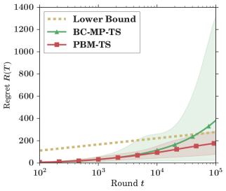
(a) Average regret of PBM-TS and BC-MP-TS compared for high parameters. Shaded areas: first and last deciles.

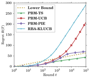
(b) Average regret of various algorithms on synthetic data under the PBM.

Figure 1: Simulation results for the suggested strategies.

5.1 Simulations

In order to evaluate our strategies, a simple problem is considered in which $K=5$, $L=3$, $\kappa=(0.9,0.6,0.3)$ and $\theta=(0.45,0.35,0.25,0.15,0.05)$. The arm expectations are chosen such that the asymptotic behavior can be observed after reasonable time horizon. All results are averaged based on $10,000$ independent runs of the algorithm. We present the results in Figure 1(b) where PBM-UCB, PBM-PIE and PBM-TS are compared to RBA-KL-UCB. The performance of PBM-PIE and PBM-TS are comparable, the latter even being under the lower bound (it is a common observation, e.g. see [12], and is due to the asymptotic nature of the lower bound). The curves confirm our analysis for PBM-PIE and lets us conjecture that the true Thompson Sampling policy might be asymptotically optimal. As expected, PBM-PIE shows asymptotically optimal performance, matching the lower bound after a large enough horizon.

$\#$ads $\boldsymbol{(K)}$	$\boldsymbol{\#}$records	$\boldsymbol{\min~{}\theta}$	$\boldsymbol{\max~{}\theta}$
$5$	$216,565$	$0.016$	$0.077$
$5$	$68,179$	$0.031$	$0.050$
$6$	$435,951$	$0.025$	$0.067$
$6$	$110,071$	$0.023$	$0.069$
$6$	$147,214$	$0.004$	$0.148$
$8$	$122,218$	$0.108$	$0.146$
$11$	$1,228,004$	$0.022$	$0.149$
$11$	$391,951$	$0.022$	$0.084$

Table 1: Statistics on the queries: each line corresponds to the sub-dataset associated with a query.

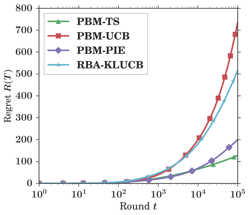
Figure 2: Performance of the proposed algorithms under the PBM on real data.

5.2 Real data experiments: search advertising

The dataset was provided for KDD Cup 2012 track 2 and involves session logs of soso.com, a search engine owned by Tencent. It consists of ads that were inserted among search results. Each of the $150M$ lines from the log contains the user ID, the query typed, an ad, a position ($1$, $2$ or $3$) at which it was displayed and a binary reward (click/no-click). First, for every query, we excluded ads that were not displayed at least $1,000$ times at every position. We also filtered queries that had less than $5$ ads satisfying the previous constraints. As a result, we obtained $8$ queries with at least $5$ and up to $11$ ads. For each query $q$, we computed the matrix of the average click-through rates (CTR): $M_{q}\in\mathds{R}^{K\times L}$, where $K$ is the number of ads for the query $q$ and $L=3$ the number of positions. It is noticeable that the SVD of each $M_{q}$ matrix has a highly dominating first singular value, therefore validating the low-rank assumption underlying in the PBM. In order to estimate the parameters of the problem, we used the EM algorithm suggested by [4, 8]. Table 1 reports some statistics about the bandit models reconstructed for each query: number of arms $K$, amount of data used to compute the parameters, minimum and maximum values of the $\theta$’s for each model.

We conducted a series of $2,000$ simulations over this dataset. At the beginning of each run, a query was randomly selected together with corresponding probabilities of scanning positions and arm expectations. Even if rewards were still simulated, this scenario is more realistic since the values of the parameters were extracted from a real-world dataset. We show results for the different algorithms in Figure 2. It is remarkable that RBA-KL-UCB performs slightly better than PBM-UCB. One can imagine that PBM-UCB does not benefit enough from position aggregations – only $3$ positions are considered – to beat RBA-KL-UCB. Both of them are outperformed by PBM-TS and PBM-PIE.

Conclusion

This work provides the first complete analysis of the PBM in an online context. The proof scheme used to obtain the lower bound on the regret is interesting on its own, as it can be generalized to various other settings. The tightness of the lower bound is validated by our analysis of PBM-PIE but it would be an interesting future contribution to provide such guarantees for more straightforward algorithms such as PBM-TS or a ‘PBM-KLUCB’ using the confidence regions of PBM-PIE. In practice, the algorithms are robust to small variations of the values of the $(\kappa_{l})_{l}$, but it would be preferable to obtain some control over the regret under uncertainty on these examination parameters.

Appendix A Properties of $\hat{\theta}_{k}(t)$ (Section 2)

Conditionnally to the actions $A(1)$ up to $A(t-1)$, the log-likelihood of the observations $Z(1),\dots,Z(t-1)$ may be written as

$$\sum_{s=}^{t-1}\sum_{k=1}^{K}\sum_{l=1}^{L}\mathds{1}\{A_{l}(t)=k\}\left[Z_{l}(t)\log(\kappa_{l}\theta_{k})+(1-Z_{l}(t))\log(1-\kappa_{l}\theta_{k})\right]\\ =\sum_{k=1}^{K}\sum_{l=1}^{L}S_{k,l}(t)\log(\kappa_{l}\theta_{k})+(N_{k,l}(t)-S_{k,l}(t))\log(1-\kappa_{l}\theta_{k}).$$

Differenciating twice with respect to $\theta_{k}$ and taking the expectation of $(S_{k,l}(t))_{l}$, contional to $A(1),\dots,A(t-1)$, yields the expression of $I(\theta_{k})$ given in Section 2.

Appendix B Proof of Theorem 4

B.1 Proof of Lemma 2

.

Under the PBM, the conditional expectation of the log-likelihood ratio defined in (4) writes

$$\mathds{E}_{\theta}[\ell(t)|A(1),\ldots,A(t)] =\mathds{E}_{\theta}\left[\sum_{s=1}^{t}\sum_{a\in\mathcal{A}}\mathds{1}\{A(s)=a\}\sum_{l=1}^{L}\log\frac{p_{a_{l}}(X_{l}(s)Y_{l}(s);\theta)}{p_{a_{l}}(X_{l}(s)Y_{l}(s);\lambda)}~{}\middle|~{}A(1),\ldots,A(t)\right]$$

$$=\sum_{s=1}^{t}\sum_{a\in\mathcal{A}}\mathds{1}\{A(s)=a\}\sum_{l=1}^{L}\mathds{E}\left[\log\frac{p_{a_{l}}(X_{l}(s)Y_{l}(s);\theta)}{p_{a_{l}}(X_{l}(s)Y_{l}(s);\lambda)}~{}\middle|~{}A(s)=a\right]$$

$$=\sum_{a\in\mathcal{A}}N_{a}(t)\sum_{l=1}^{L}\sum_{k=1}^{K}\mathds{1}\{a_{l}=k\}d(\kappa_{l}\theta_{k},\kappa_{l}\lambda_{k})$$

$$=\sum_{a\in\mathcal{A}}N_{a}(t)I_{a}(\theta,\lambda),$$

using the notation $I_{a}(\theta,\lambda)=\sum_{l=1}^{L}\sum_{k=1}^{K}\mathds{1}\{a_{l}=k\}d(\kappa_{l}\theta_{k},\kappa_{l}\lambda_{k})$. ∎

B.2 Details on the proof of Proposition 3

Lemma 12.

Let $\theta=(\theta_{1},\ldots,\theta_{K})$ and $\lambda=(\lambda_{1},\ldots,\lambda_{K})$ be two bandit models such that the distributions of all arms in $\theta$ and $\lambda$ are mutually absolutely continuous. Let $\sigma$ be a stopping time with respect to $(\mathcal{F}_{t})$ such that $(\sigma<+\infty)$ a.s. under both models. Let $\mathcal{E}\in\mathcal{F}_{\sigma}$ be an event such that $0<\mathds{P}_{\theta}(\mathcal{E})<1$. Then one has

$$\sum_{a\in\mathcal{A}}I_{a}(\theta,\lambda)\mathds{E}_{\theta}[N_{a}(\sigma)]\geq d(\mathds{P}_{\theta}(\mathcal{E}),\mathds{P}_{\lambda}(\mathcal{E})),$$

where $I_{a}(\theta,\lambda)$ is the conditional expectation of the log-likelihood ratio for the model of interest.

The proof of this lemma directly follows from the above expressions of the log-likelihood ratio and from the proof of Lemma $1$ in Appendix A.1 of [11].

We simply recall the following technical lemma for completeness.

Lemma 13.

Let $\sigma$ be any stopping time with respect to $(\mathcal{F}_{t})$. For every event $A\in\mathcal{F}_{\sigma}$,

$$\mathds{P}_{\lambda}(A)=\mathds{E}_{\theta}[\mathds{1}\{A\}\exp(-\ell(\sigma))].$$

A full proof of Lemma 13 can be found in the Appendix A.3 of [11] (proof of Lemma 15).

B.3 Lower bound proof (Theorem 4)

.

In order to prove the simplified lower bound of Theorem 4 we basically have two arguments:

1. a lower bound on $f(\theta)$ can be obtained by enlarging the feasible set, that is by relaxing some constraints;

2. Lemma 15 can be used to lower bound the objective function of the problem.

The constant $f(\theta)$ is defined by

$$f(\theta)=\inf_{c\succeq 0}\sum_{a\neq a^{*}(\theta)}\Delta_{a}(\theta)c_{a}$$ (8)

$$s.t~{}~{}\inf_{\lambda\in B(\theta)}\sum_{a\in\mathcal{A}}I_{a}(\theta,\lambda)c_{a}\geq 1.$$ (9)

We begin by relaxing some constraints: we only allow the change of measure $\lambda$ to belong to the sets $B_{k}(\theta):=\left\{\lambda\in\Theta|\forall j\neq k,\theta_{j}=\lambda_{j}\text{ and }\mu^{*}(\theta)<\mu^{*}(\lambda)\right\}$ defined in Section 3:

$$f(\theta)=\inf_{c\succeq 0}\sum_{a\neq a^{*}(\theta)}\Delta_{a}(\theta)c_{a}$$ (10)

$$s.t~{}~{}\forall k\notin a^{*}(\theta),~{}\forall\lambda\in B_{k}(\theta),\sum_{a\in\mathcal{A}}I_{a}(\theta,\lambda)c_{a}\geq 1.$$ (11)

The $K-L$ constraints (11) only let one parameter move and must be true for any value satisfying the definition of the corresponding set $B_{k}(\theta)$. In practice, for each $k$, the parameter $\lambda_{k}$ must be set to at least $\theta_{L}$. Consequently, these constraints may then be rewritten

$$f(\theta)=\inf_{c\succeq 0}\sum_{a\neq a^{*}(\theta)}\Delta_{a}(\theta)c_{a}$$ (12)

$$s.t~{}\forall k\notin a^{*}(\theta),\sum_{a\neq a^{*}(\theta)}c_{a}\sum_{l=1}^{L}\mathds{1}\{a_{l}=k\}d(\kappa_{l}\theta_{k},\kappa_{l}\theta_{L})\geq 1.$$ (13)

Proposition 14 tells us that coefficients $c_{a}$ are all zeros except for actions $a\in\mathcal{A}$ which can be written $a=v_{k,l_{k}}$ where $l_{k}=\operatorname*{arg\,min}_{l\leq L}\frac{\Delta_{v_{k,l}}(\theta)}{d(\kappa_{l}\theta_{k},\kappa_{l}\theta_{L})}$. Thus, we obtain the desired lower bound by rewriting (12) as

$$f(\theta)\geq\sum_{k=L+1}^{K}\min_{l\in\{1,\ldots,L\}}\frac{\Delta_{v_{k,l}}(\theta)}{d(\kappa_{l}\theta_{k},\kappa_{l}\theta_{L})}.$$

∎

Proposition 14.

Let $c=\{c_{a}~{}:~{}a\neq a^{*}\}$ be a solution of the linear problem (LP) in Theorem 4. Coefficients are all zeros except for actions $a$ which can be written as $a=(1,\ldots,l_{k}-1,k,l_{k},\ldots,L-1):=v_{k,l_{k}}$ where $k>L$ and $l_{k}=\operatorname*{arg\,min}_{l\leq L}\frac{\Delta_{v_{k,l}}(\theta)}{d(\kappa_{l}\theta_{k},\kappa_{l}\theta_{L})}$.

Proof.

We denote by $\pi_{k}(a)$ the position of item $k\in\{1,\ldots,K\}$ in action $a$ ($0$ if $k\notin a$). Let $l_{k}$ be the optimal position of item $k>L$ for exploration: $l_{k}=\operatorname*{arg\,min}_{l\leq L}\frac{\Delta_{v_{k,l}}(\theta)}{d(\kappa_{l}\theta_{k},\kappa_{l}\theta_{L})}$. Following [5], we show by contradiction that $c_{a}>0$ implies that $a$ can be written $v_{k,l_{k}}$ for a well chosen $k>L$. Let $\alpha\neq a^{*}$ be a suboptimal action such that $\forall k>L,\alpha\neq v_{k,l_{k}}$ and $c_{\alpha}>0$. We need to show a contradiction. Let us introduce a new set of coefficients $c^{\prime}$ defined as follows, for any $a\neq a^{*}$:

$$c^{\prime}_{a}=\begin{cases}0&\quad\text{if }a=\alpha\\ c_{a}+\frac{d(\kappa_{\pi_{k}(\alpha)}\theta_{k},\kappa_{\pi_{k}(\alpha)}\theta_{L})}{d(\kappa_{l_{k}}\theta_{k},\kappa_{l_{k}}\theta_{L})}c_{\alpha}&\quad\text{if }\exists k>L\text{ s.t. }a=v_{k,l_{k}}\text{ and }k\in\alpha\\ c_{a}\ &\quad\text{otherwise.}\\ \end{cases}$$

According to Lemma 15, these coefficients satisfy the constraints of the LP. We now show that these new coefficients yield a strictly lower value to the optimization problem:

$$c(\theta)-c^{\prime}(\theta) =c_{\alpha}\Delta_{\alpha}(\theta)-\sum_{k>L:k\in\alpha}\frac{d(\kappa_{\pi_{k}(\alpha)}\theta_{k},\kappa_{\pi_{k}(\alpha)}\theta_{L})}{d(\kappa_{l_{k}}\theta_{k},\kappa_{l_{k}}\theta_{L})}c_{\alpha}\Delta_{v_{k,l_{k}}}(\theta)$$

$$>c_{\alpha}\left(\sum_{k>L:k\in\alpha}\Delta_{v_{k,\pi_{k}(\alpha)}}(\theta)-\sum_{k>L:k\in\alpha}\frac{d(\kappa_{\pi_{k}(\alpha)}\theta_{k},\kappa_{\pi_{k}(\alpha)}\theta_{L})}{d(\kappa_{l_{k}}\theta_{k},\kappa_{l_{k}}\theta_{L})}\Delta_{v_{k,l_{k}}}(\theta)\right).$$ (14)

The strict inequality (14) is shown in Lemma 16. Let $k>L$ be one of the suboptimal arms in $\alpha$. By definition of $l_{k}$, the corresponding term of the sum in equation (14) is positive. Thus, we have that $c(\theta)>c^{\prime}(\theta)$ and, hence, by contradiction, we showed that $c_{a}>0$ iff $a$ can be written $a=v_{k,l_{k}}$ for some $k>L$. ∎

Lemma 15.

Let $c$ be a vector of coefficients that satisfy constraints (13) of the optimization problem. Then, coefficients $c^{\prime}$ as defined in Proposition 14 also satisfy the constraints:

$$\forall k\notin a^{*}(\theta),\sum_{a\neq a^{*}(\theta)}c^{\prime}_{a}\sum_{l=1}^{L}\mathds{1}\{a_{l}=k\}d(\kappa_{l}\theta_{k},\kappa_{l}\theta_{L})\geq 1.$$

Proof.

We use the same $\alpha$ as introduced in Proposition 14. Let us fix $k\notin a^{*}(\theta)$. Let us define

$$L(c)=\sum_{a\neq a^{*}(\theta)}c_{a}\sum_{l=1}^{L}\mathds{1}\{a_{l}=k\}d(\kappa_{l}\theta_{k},\kappa_{l}\theta_{L}).$$

We have

$$L(c^{\prime})-L(c)=-c_{\alpha}\sum_{l=1}^{L}\mathds{1}\{\alpha_{l}=k\}d(\kappa_{l}\theta_{k},\kappa_{l}\theta_{L})+\sum_{l:\alpha_{l}>L} \frac{d(\kappa_{l}\theta_{k},\kappa_{l}\theta_{L})}{d(\kappa_{l_{k}}\theta_{k},\kappa_{l_{k}}\theta_{L})}c_{\alpha}$$

$$\times\mathds{1}\{\alpha_{l}=k\}d(\kappa_{l_{k}}\theta_{k},\kappa_{l_{k}}\theta_{L}).$$

If $k\notin\alpha$, clearly, $L(c^{\prime})-L(c)=0$. Else, $k\in\alpha$ and we note $p$ its position in $\alpha$: $p=\pi_{k}(\alpha)$. We rewrite:

$$L(c^{\prime})-L(c)=c_{\alpha}d(\kappa_{p}\theta_{k},\kappa_{p}\theta_{L})\left(-1+\frac{d(\kappa_{l_{k}}\theta_{k},\kappa_{l_{k}}\theta_{L})}{d(\kappa_{l_{k}}\theta_{k},\kappa_{l_{k}}\theta_{L})}\right)=0.$$

Thus, the coefficients $c^{\prime}$ satisfy the constraints from Proposition 14. ∎

Lemma 16.

Let $\alpha$ be as in the proof of Proposition 14.

$$\Delta_{\alpha}(\theta)>\sum_{k>L:k\in\alpha}\Delta_{v_{k,\pi_{k}(\alpha)}}(\theta).$$

Proof.

Let $k_{1},\ldots,k_{p}$ be the suboptimal arms in $\alpha$ by increasing position. Let $v(\alpha)$ be the action in $\mathcal{A}$ with lower regret such that it contains all the suboptimal arms of $\alpha$ in the same positions. Thus, $v(\alpha)=(1,\ldots,\pi_{k_{1}}(\alpha)-1,k_{1},\pi_{k_{1}}(\alpha),\ldots,\pi_{k_{2}}(\alpha)-2,k_{2},\pi_{k_{2}}(\alpha)-1,\ldots,L-p)$. By definition, one has that $\Delta_{\alpha}(\theta)\geq\Delta_{v(\alpha)}(\theta)$. In the following, we show that $\Delta_{v(\alpha)}(\theta)\geq\sum_{k>L:k\in\alpha}\Delta_{v_{k,\pi_{k}(\alpha)}}(\theta)$ for $p=2$ (that is to say $\alpha$ contains $2$ suboptimal arms $k_{1}$ and $k_{2}$).

For the sake of readability, we write $\pi_{i}$ instead of $\pi_{k_{i}}(\alpha)$ in the following.

$$\Delta_{v(\alpha)}(\theta) =\sum_{l=1}^{L}\kappa_{l}(\theta_{l}-\theta_{(v_{k_{1},\pi_{1}})_{l}})+\sum_{l=1}^{L}\kappa_{l}(\theta_{(v_{k_{1},\pi_{1}})_{l}}-\theta_{v(\alpha)_{l}})$$

$$=\Delta_{v_{k_{1},\pi_{1}}}(\theta)+\left[\kappa_{\pi_{2}}\theta_{\pi_{2}-1}+\ldots+\kappa_{L}\theta_{L-1}\right]-\left[\kappa_{\pi_{2}}\theta_{k_{2}}+\kappa_{\pi_{2}+1}\theta_{\pi_{2}-1}+\ldots+\kappa_{L}\theta_{L-2}\right]$$

$$=\Delta_{v_{k_{1},\pi_{1}}}(\theta)+\Delta_{v_{k_{2},\pi_{2}}}(\theta)+\left[\kappa_{\pi_{2}}(\theta_{\pi_{2}-1}-\theta_{\pi_{2}})+\ldots+\kappa_{L}(\theta_{L-1}-\theta_{L})\right]-$$

$$~{}~{}~{}~{}\left[\kappa_{\pi_{2}+1}(\theta_{\pi_{2}-1}-\theta_{\pi_{2}})+\ldots+\kappa_{L}(\theta_{L-2}-\theta_{L-1})\right]$$

$$=\Delta_{v_{k_{1},\pi_{1}}}(\theta)+\Delta_{v_{k_{2},\pi_{2}}}(\theta)+\mathcal{R}(\theta).$$

Thus, one has to show that $\mathcal{R}(\theta)=\kappa_{\pi_{2}}(\theta_{\pi_{2}-1}-\theta_{\pi_{2}})+\kappa_{\pi_{2}+1}(2\theta_{\pi_{2}}-\theta_{\pi_{2}-1}-\theta_{\pi_{2}+1})+\ldots+\kappa_{L}(2\theta_{L-1}-\theta_{L-2}-\theta_{L})>0$. In fact, using that $\kappa_{l}\geq\kappa_{l+1}$ for all $l<L$, we have

$$\mathcal{R}(\theta) \geq\kappa_{\pi_{2}+1}(\theta_{\pi_{2}-1}-\theta_{\pi_{2}}+2\theta_{\pi_{2}}-\theta_{\pi_{2}-1}-\theta_{\pi_{2}+1})+\ldots+\kappa_{L}(2\theta_{L-1}-\theta_{L-2}-\theta_{L})$$

$$\geq\kappa_{\pi_{2}+2}(\theta_{\pi_{2}+1}-\theta_{\pi_{2}+2})+\ldots+\kappa_{L}(2\theta_{L-1}-\theta_{L-2}-\theta_{L})$$

$$\geq\ldots$$

$$\geq\kappa_{L}(\theta_{L-1}-\theta_{L})$$

$$>0.$$

∎

Appendix C Proof of Proposition 8

In this section, we fix an arm $k\in\{1,\dots,K\}$ and obtain an upper confidence bound for the estimator $\hat{\theta}_{k}(t):=S_{k}(t)/\tilde{N}_{k}(t)$. Let $\tau_{i}$ be the instant of the $i$-th draw of arm $k$ (the $\tau_{i}$ are stopping times w.r.t. $\mathcal{F}_{t}$). We introduce the centered sequence of successive observations from arm $k$

$$\bar{Z}_{k,i}=\sum_{l=1}^{L}\mathds{1}\{A_{l}(\tau_{i})=k\}(X_{l}(\tau_{i})Y_{l}(\tau_{i})-\theta_{k}\kappa_{l}).$$ (15)

Introducing the filtration $\mathcal{G}_{i}=\mathcal{F}_{\tau_{i+1}-1}$, one has $\mathds{E}[\bar{Z}_{k,i}|\mathcal{G}_{i-1}]=0$, and therefore, the sequence

$$M_{k,n}=\sum_{i=1}^{n}\bar{Z}_{k,i}$$

is a martingale with bounded increments, w.r.t. the filtration $(\mathcal{G}_{n})_{n}$. By construction, one has

$$M_{k,N_{k}(t)}=S_{k}(t)-\tilde{N}_{k}(t)\theta_{k}=\tilde{N}_{k}(t)(\hat{\theta}_{k}(t)-\theta_{k}).$$

We use the so-called peeling technique together with the maximal version of Azuma-Hoeffding’s inequality [2]. For any $\gamma>0$ one has

$$\mathds{P}\left(M_{k,N_{k}(t)}<-\sqrt{N_{k}(t)\delta/2}\right) \leq\sum_{i=1}^{\frac{\log(t)}{\log(1+\gamma)}}\mathds{P}\left(M_{k,N_{k}(t)}<-\sqrt{N_{k}(t)\delta/2}\,,N_{k}(t)\in[(1+\gamma)^{i-1},(1+\gamma)^{i})\right)$$

$$\leq\sum_{i=1}^{\frac{\log(t)}{\log(1+\gamma)}}\mathds{P}\left(\exists i\in\{1,\dots,(1+\gamma)^{i}\}:\ M_{k,i}<-\sqrt{(1+\gamma)^{i-1}\delta/2}\right)$$

$$\leq\sum_{i=1}^{\frac{\log(t)}{\log(1+\gamma)}}\exp\left(-\frac{\delta(1+\gamma)^{i-1}}{(1+\gamma)^{i}}\right)=\frac{\log(t)}{\log(1+\gamma)}\exp\left(-\frac{\delta}{(1+\gamma)}\right).$$

Choosing $\gamma=1/(\delta-1)$, gives

$$\mathds{P}\left(\hat{\theta}_{k}(t)-\theta_{k}<-\frac{\sqrt{N_{k}(t)\delta/2}}{\tilde{N}_{k}(t)}\right)\leq\delta e\log(t)e^{-\delta}.$$

Appendix D Regret analysis for PBM-UCB (Theorem 9)

We proceed as Kveton et al. (2015) [14]. We start by considering separately rounds when one of the confidence intervals is violated. We denote by $B_{t,k}=\sqrt{N_{k}(t)(1+\epsilon)\log t/2}/\tilde{N}_{k}(t)$ the PBM-UCB exploration bonus and by $B_{t,k}^{+}=\sqrt{N_{k}(t)(1+\epsilon)\log T/2}/\tilde{N}_{k}(t)$ an upper bound of this bonus (for $t\leq T$). We define the event $E_{t}=\{\exists k\in A(t)\,:\,|\hat{\theta}_{k}(t)-\theta_{k}|>B_{t,k}\}$. Then, the regret can be decomposed into

$$R(T)=\sum_{t=1}^{T}\Delta_{A(t)}\mathds{1}_{E_{t}}+\Delta_{A(t)}\mathds{1}_{\bar{E_{t}}}.$$

and, similarly to [14] (Appendix A.1), the first term of this sum can be bounded from above in expectation by a constant $C_{0}(\epsilon)$ that does not depend on $T$ using Proposition 8. So, it remains to bound the regret suffered even when confidence intervals are respected, that is the sum on the r.h.s of

$$\mathbb{E}[R(T)]<C_{0}(\epsilon)+\mathbb{E}[\sum_{t=1}^{T}\Delta_{A(t)}\mathds{1}\{\bar{E_{t}},\Delta_{A(t)}>0\}].$$

It can be done using techniques from [6, 14]. We start by defining events $F_{t}$, $G_{t}$, $H_{t}$ in order to decompose the part of the regret at stake. Then, we show an equivalent of Lemma 2 of [14] for our case and finally we refer to the proof of Theorem 3 in Appendix A.3 of [14].

For each round $t\geq 1$, we define the set of arms $S_{t}=\{1\leq l\leq L:N_{A_{l}(t)}(t)\leq\frac{8(1+\epsilon)\log T\left(\sum_{s=1}^{L}\kappa_{s}\right)^{2}}{\kappa_{L}^{2}\Delta_{A(t)}^{2}}\}$ and the related events

• $F_{t}=\{\Delta_{A(t)}>0,\,\Delta_{A(t)}\leq 2\sum_{l=1}^{L}\kappa_{l}B_{t,A_{l}(t)}^{+}\}$;

• $G_{t}=\{|S_{t}|\geq l\}$;

• $H_{t}=\{|S_{t}|<l\,,\,\exists k\in A(t),N_{k}(t)\leq\frac{8(1+\epsilon)\log T\left(\sum_{s=1}^{l}\kappa_{s}\right)^{2}}{\kappa_{L}^{2}\Delta_{A(t)}^{2}}\}$, where the constraint on $N_{k}(t)$ only differs from the first one by its numerator which is smaller than the previous one, leading to an even stronger constraint.

Fact 17.

According to Lemma 1 in [14], the following inequality is still valid with our own definition of $F_{t}$ :

$$\sum_{t=1}^{T}\Delta_{A(t)}\mathds{1}\{\bar{E_{t}},\Delta_{A(t)}>0\}\leq\sum_{t=1}^{T}\Delta_{A(t)}\mathds{1}\{F_{t}\}.$$

Proof.

Invoking Lemma 1 from [14] needs to be justified as our setting is quite different. Taking action $A(t)$ means that

$$\sum_{l=1}^{L}\kappa_{l}U_{A_{l}(t)}(t)\geq\sum_{l=1}^{L}\kappa_{l}U_{l}(t).$$

Under event $\bar{E}_{t}$, all UCB’s are above the true parameter $\theta_{k}$ so we have

$$\sum_{l=1}^{L}\kappa_{l}(\theta_{A_{l}(t)}+2B_{t,A_{l}(t)})\geq\sum_{l=1}^{L}\kappa_{l}(\theta_{l}+B_{t,l})\geq\sum_{l=1}^{L}\kappa_{l}\theta_{l}.$$

Rearranging the terms above and using $B_{t,l(t)}\leq B_{t,l(t)}^{+}$, we obtain

$$\sum_{l=1}^{L}\kappa_{l}B_{t,A_{l}(t)}^{+}\geq 2\sum_{l=1}^{L}\kappa_{l}B_{t,A_{l}(t)}\geq\Delta_{A(t)}.$$

∎

We now have to prove an equivalent of Lemma 2 in [6] that would allow us to split the right-hand side above in two parts. Let us show that $F_{t}\subset(G_{t}\cup H_{t})$ by showing its contrapositive: if $F_{t}$ is true then we cannot have $(\bar{G_{t}}\cap\bar{H_{t}})$. Assume both of these events are true. Then, we have

$$\Delta_{A(t)} \overset{F_{t}}{\leq}2\sum_{l=1}^{L}\kappa_{l}B_{t,A_{l}(t)}^{+}$$

$$\leq 2\sum_{l=1}^{L}\kappa_{l}\sqrt{\frac{N_{A_{l}(t)}(t)}{\tilde{N}_{A_{l}(t)}(t)}}\sqrt{\frac{(1+\epsilon)\log(T)}{2\tilde{N}_{A_{l}(t)}(t)}}$$

$$=2\sum_{l=1}^{L}\kappa_{l}\frac{N_{A_{l}(t)}(t)}{\tilde{N}_{A_{l}(t)}(t)}\sqrt{\frac{(1+\epsilon)\log(T)}{2N_{A_{l}(t)}(t)}}$$

$$\leq\frac{\sqrt{2(1+\epsilon)\log T}}{\kappa_{L}}\sum_{l=1}^{L}\frac{\kappa_{l}}{\sqrt{N_{A_{l}(t)}(t)}}$$

$$=\frac{\sqrt{2(1+\epsilon)\log T}}{\kappa_{L}}\left(\sum_{l\notin S_{t}}\frac{\kappa_{l}}{\sqrt{N_{A_{l}(t)}(t)}}+\sum_{l\in S_{t}}\frac{\kappa_{l}}{\sqrt{N_{A_{l}(t)}(t)}}\right)$$

$$\overset{(\bar{G_{t}}\cap\bar{H_{t}})}{<}\frac{\sqrt{2(1+\epsilon)\log T}}{\kappa_{L}}\frac{\kappa_{L}\Delta_{A(t)}}{2\sqrt{2(1+\epsilon)\log T}}\left(\frac{\sum_{l\notin S_{t}}\kappa_{l}}{\sum_{s=1}^{L}\kappa_{s}}+\frac{\sum_{l\in S_{t}}\kappa_{l}}{\sum_{s=1}^{l}\kappa_{s}}\right)$$

$$\leq\Delta_{A(t)}$$

which is a contradiction. The end of the proof proceeds exactly as in the end of the proof of Theorem 6 in of [6]: events $G_{t}$ and $H_{t}$ are split into subevents corresponding to rounds where each specific suboptimal arm of the list is in $S_{t}$ or verifies the condition of $H_{t}$. We define

$$G_{k,t} =G_{t}\cap\{k\in A(t),\,N_{k}(t)\leq\frac{8(1+\epsilon)\log T\left(\sum_{s=1}^{L}\kappa_{s}\right)^{2}}{\kappa_{L}^{2}\Delta_{A(t)}^{2}}\ \},$$

$$H_{k,t} =H_{t}\cap\{k\in A(t),\,N_{k}(t)\leq\frac{8(1+\epsilon)\log T\left(\sum_{s=1}^{l}\kappa_{s}\right)^{2}}{\kappa_{L}^{2}\Delta_{A(t)}^{2}}\}.$$

The way we defined these subevents allows to write the two following bounds :

$$\sum_{k=1}^{K}\mathds{1}\{G_{k,t}\}=\mathds{1}\{G_{t}\}\sum_{k=1}^{K}\mathds{1}\{k\in S_{t}\}\geq l\mathds{1}\{G_{t}\}$$

so $\mathds{1}\{G_{t}\}\leq\sum_{k}\mathds{1}\{G_{k,t}\}/l$. And,

$$\mathds{1}\{H_{t}\}\leq\sum_{k=1}^{K}\mathds{1}\{H_{k,t}\}.$$

We can now bound the regret using these two results:

$$\sum_{t=1}^{T}\Delta_{A(t)}(\mathds{1}\{G_{t}\}+\mathds{1}\{H_{t}\}) \leq\sum_{t=1}^{T}\sum_{k=1}^{K}\frac{\Delta_{A(t)}}{l}\mathds{1}\{G_{k,t}\}+\sum_{t=1}^{T}\sum_{k=1}^{K}\Delta_{A(t)}\mathds{1}\{H_{k,t}\}$$

$$=\sum_{t=1}^{T}\sum_{k=1}^{K}\frac{\Delta_{A(t)}}{l}\mathds{1}\{G_{k,t},A(t)\neq a^{*}\}+\sum_{t=1}^{T}\sum_{k=1}^{K}\Delta_{A(t)}\mathds{1}\{H_{k,t},A(t)\neq a^{*}\}.$$

For each arm $k$, there is a finite number $C_{k}:=|\mathcal{A}_{k}|$ of actions in $\mathcal{A}$ containing $k$; we order them such that the corresponding gaps are in decreasing order $\Delta_{k,1}\geq\ldots\geq\Delta_{k,C_{k}}>0$. So we decompose each sum above on the different actions $A(t)$ possible:

$$\ldots \leq\sum_{t=1}^{T}\sum_{k=1}^{K}\sum_{a\in\mathcal{A}_{k}}\frac{\Delta_{k,a}}{l}\mathds{1}\{G_{k,t},A(t)=a\}+\sum_{t=1}^{T}\sum_{k=1}^{K}\sum_{a\in\mathcal{A}_{k}}\Delta_{k,a}\mathds{1}\{H_{k,t},A(t)=a\}.$$

The two sums on the right hand side look alike. For arm $k$ fixed, events $G_{k,t}$ and $H_{k,t}$ imply almost the same condition on $N_{k}(t)$, only $H_{k,t}$ is stronger because the bounding term is smaller. We now rely on a technical result by [6] that allows to bound each sum.

Lemma 18.

([6], Lemma 2 in Appendix B.4) Let $k$ be a fixed item and $|\mathcal{A}_{k}|\geq 1$, $C>0$, we have

$$\sum_{t=1}^{T}\sum_{a\in\mathcal{A}_{k}}\mathds{1}\{k\in A(t),\,N_{k}(t)\leq C/\Delta_{k,a}^{2},\,A(t)=a\}\Delta_{k,a}\leq\frac{2C}{\Delta_{\text{min},k}}$$

where $\Delta_{\text{min},k}$ is the smallest gap among all suboptimal actions containing arm $k$. In particular, when $k\notin a^{*}$ the smallest gap is $\Delta_{\text{min},k}=\kappa_{L}(\theta_{L}-\theta_{k})$. While, when $k\in a^{*}$ it is less obvious what the minimal gap is, however it corresponds the second best action $A_{2}$ containing only optimal arms: $\Delta_{\text{min},k}=\Delta_{A_{2}}$.

So, bounding each sum with the above lemma, we obtain

$$\sum_{t=1}^{T}\Delta_{A(t)}(\mathds{1}\{G_{t}\}+\mathds{1}\{H_{t}\})\leq\frac{16(1+\epsilon)\log T}{\kappa_{L}^{2}}\underbrace{\left(\frac{\left(\sum_{s=1}^{L}\kappa_{s}\right)^{2}}{l}+\left(\sum_{s=1}^{l}\kappa_{s}\right)^{2}\right)}_{C(l;\kappa)}\left(\frac{L}{\Delta_{A_{2}}}+\sum_{k\notin a^{*}}\frac{1}{\kappa_{L}(\theta_{L}-\theta_{k})}\right).$$

This bound can be optimized by minimizing $C(l;\kappa)$ over $l$.

Appendix E Regret analysis for PBM-PIE (Theorem 11)

The proof follows the decomposition of [5]. For all $t\geq 1$, we denote $f(t,\epsilon)=(1+\epsilon)\log t$.

E.1 Controlling leaders and estimations

Define $\eta_{0}=\min_{k\in\{1,\ldots,L-1\}}(\theta_{k}-\theta_{k+1})/2$ and let $\eta<\eta_{0}$. We define the following set of rounds

$$A=\{t\geq 1:\mathcal{L}(t)\neq(1,\ldots,L)\}.$$

Our goal is to upper bound the expected size of $A$. Let us introduce the following sets of rounds:

$$B =\{t\geq 1:\exists k\in\mathcal{L}(t),|\hat{\theta}_{k}(t)-\theta_{k}|\geq\eta\},$$

$$C =\{t\geq 1:\exists k\leq L,U_{k}(t)\leq\theta_{k}\},$$

$$D =\{t\geq 1:t\in A\setminus(B\cup C),\exists k\leq L,k\notin\mathcal{L}(t),|\hat{\theta}_{k}(t)-\theta_{k}|\geq\eta\}.$$

We first show that $A\subset(B\cup C\cup D)$. Let $t\in A\setminus(B\cup C)$. Let $k,k^{\prime}\in\mathcal{L}(t)$ such that $k<k^{\prime}$. Since $t\notin B$, we have that $|\hat{\theta}_{k}(t)-\theta_{k}|\leq\eta$ and $|\hat{\theta}_{k^{\prime}}(t)-\theta_{k^{\prime}}|\leq\eta$. Since $\eta\leq(\theta_{k}-\theta_{k^{\prime}})/2$, we conclude that $\hat{\theta}_{k}(t)\geq\hat{\theta}_{k^{\prime}}(t)$. This proves that $(\mathcal{L}_{1}(t),\ldots,\mathcal{L}_{L}(t)$ is an increasing sequence. We have that $\mathcal{L}_{L}(t)>L$ otherwise $\mathcal{L}(t)=(1,\ldots,L)$ which is a contradiction because $t\in A$. Since $\mathcal{L}_{L}(t)>L$, there exists $k\leq L$ such that $k\notin\mathcal{L}(t)$. We show by contradiction that $|\hat{\theta}_{k}(t)-\theta_{k}|\geq\eta$. Assume that $|\hat{\theta}_{k}(t)-\theta_{k}|\leq\eta$. We also have that $\hat{\theta}_{\mathcal{L}_{L}(t)}(t)-\theta_{\mathcal{L}_{L}(t)}\leq\eta$ because $\mathcal{L}_{L}(t)\in\mathcal{L}(t)$ and $t\notin B$. Thus, $\hat{\theta}_{k}(t)>\hat{\theta}_{\mathcal{L}_{L}(t)}(t)$. We have a contradiction because this would imply that $k\in\mathcal{L}(t)$. Finally we have proven that if $t\in A\setminus(B\cup C)$, then $t\in D$ so $A\subset(B\cup C\cup D)$.

By a union bound, we obtain

$$\mathds{E}[|A|]\leq\mathds{[}|B|]+\mathds{[}|C|]+\mathds{[}|D|].$$

In the following, we upper bound each set of rounds individually.

Controlling $\mathds{E}[|B|]$:

We decompose $B=\bigcup_{k=1}^{K}(B_{k,1}\cup B_{k,2})$ where

$$B_{k,1}=\{t\geq 1:k\in\mathcal{L}(t),\mathcal{L}_{L}(t)\neq k,|\hat{\theta}_{k}(t)-\theta_{k}|\geq\eta\}$$

$$B_{k,2}=\{t\geq 1:k\in\mathcal{L}(t),\mathcal{L}_{L}(t)=k,|\hat{\theta}_{k}(t)-\theta_{k}|\geq\eta\}$$

Let $t\in B_{k,1}$: $k\in A(t)$ so $\mathds{E}[k\in A(t)|t\in B_{k,1}]=1$. Furthermore, for all $t$, $\mathds{1}\{t\in B_{k,1}\}$ is $\mathcal{F}_{t-1}$ measurable. Then we can apply Lemma 22 (with $H=B_{k,1}$ and $c=1$).

$$\mathds{E}[|B_{k,1}|]\leq 2(2+\kappa_{L}^{-2}\eta^{-2}).$$

Let $t\in B_{k,2}$: $k\in\mathcal{B}(t)$ but because of the randomization of the algorithm, $k\in A(t)$ with probability $1/2$, i.e. $\mathds{E}[k\in A(t)|t\in B_{k,2}]\geq 1/2$. We get

$$\mathds{E}[|B_{k,2}|]\leq 4(4+\kappa_{L}^{-2}\eta^{-2})$$

By union bound over $k$, we get $\mathds{E}[|B|]\leq 2K(10+3\kappa_{L}^{-2}\eta^{-2})$.

Controlling $\mathds{E}[|C|]$:

We decompose $C=\bigcup_{k=1}^{L}C_{k}$ where $C_{k}=\{t\geq 1:U_{k}(t)\leq\theta_{k}\}$

We first require to prove Proposition 10.

Proof.

Theorem 2 of [16] implies that

$$\mathbb{P}\left(\sum_{l=1}^{L}N_{k,l}(t)d(\frac{S_{k,l}(t)}{N_{k,l}(t)},\kappa_{l}\theta_{k})\geq\delta\right)\leq e^{-\delta}\left(\frac{\left\lceil\delta\log(t)\right\rceil\delta}{L}\right)^{L}e^{L+1}.$$

The function $\Phi:x\to\sum_{l=1}^{L}N_{k,l}(t)d\left(\frac{S_{k,l}(t)}{N_{k,l}(t)},\kappa_{l}x\right)$ is convex and non-decreasing on $[\theta_{k}^{min}(t),1]$; the convexity is easily checked and $\theta_{k}^{min}(t)$ is defined as the minimum of this convex function. By definition, we have, either, $U_{k}(t,\delta)=1$ and then $U_{k}(t,\delta)>\theta_{k}$, or, $U_{k}(t,\delta)<1$ and $\Phi(U_{k}(t,\delta))=\delta$, consequently

$$\mathbb{P}\left(U_{k}(t,\delta)<\theta_{k}\right)=\mathbb{P}\left(\Phi(U_{k}(t,\delta))\leq\Phi(\theta_{k})\right)=\mathbb{P}\left(\delta\leq\Phi(\theta_{k})\right).$$

∎

Remember that $U_{k}(t)=U_{k}(t,(1+\epsilon)\log(t))=U_{k}(t,f(t,\epsilon))$. Thus, applying Proposition 10, we obtain for arm $k$,

$$\mathds{E}[|C_{k}|]\leq\sum_{t=1}^{\infty}\mathds{P}(U_{k}(t)\leq\theta_{k})\leq\lceil e^{L+1}\rceil+\frac{e^{L+1}}{L^{L}}\sum_{t=\lceil e^{L+1}\rceil+1}^{\infty}\frac{(2+\epsilon)^{2L}(\log t)^{3L}}{t^{1+\epsilon}}\leq C_{3}(\epsilon),$$

for some constant $C_{3}(\epsilon)$.

Controlling $\mathds{E}[|D|]$:

Decompose $D$ as $D=\bigcup_{k=1}^{L}D_{k}$ where

$$D_{k}=\{t\geq 1:t\in A\setminus(B\cup C),k\notin\mathcal{L}(t),|\hat{\theta}_{k}(t)-\theta_{k}|\geq\eta\}.$$

For a given $k\leq L$, $D_{k}$ is the set of rounds at which $k$ is not one of the leaders, and is not accurately estimated. Let $t\in D_{k}$. Since $k\notin\mathcal{L}(t)$, we must have $\mathcal{L}_{L}(t)>L$. In turn, since $t\notin B$, we have $|\hat{\theta}_{\mathcal{L}_{L}(t)}(t)-\theta_{\mathcal{L}_{L}(t)}|\leq\eta$, so that

$$\hat{\theta}_{\mathcal{L}_{L}(t)}\leq\theta_{\mathcal{L}_{L}(t)}+\eta\leq\theta_{L}+\eta\leq(\theta_{L}+\theta_{L+1})/2.$$

Furthermore, since $t\notin C$ and $1\leq k\leq L$, we have $U_{k}(t)\geq\theta_{k}\geq\theta_{L}\geq(\theta_{L}+\theta_{L+1})/2\geq\hat{\theta}_{\mathcal{L}_{L}(t)}$. This implies that $k\in\mathcal{B}(t)$ thus $\mathds{E}[k\in A(t)|t\in D_{k}]\geq 1/(2K)$. We apply Lemma 22 with $H\equiv D_{k}$ and $c=1/(2K)$ to get

$$\mathds{E}[|D|]\leq\sum_{k=1}^{L}\mathds{E}[|D_{k}|]\leq 4K(4K+\kappa_{L}^{-2}\eta^{-2}).$$

E.2 Regret decomposition

We decompose the regret by distinguishing rounds in $A\cup B$ and other rounds. More specifically, we introduce the following sets of rounds for arm $k>L$:

$$E_{k}=\{t\geq 1:t\notin(B\cup C\cup D),\mathcal{L}(t)=a^{*},A(t)=v_{k,L}\}.$$

The set of instants at which a suboptimal action is selected now can be expressed as follows

$$\{t\geq 1:A(t)\neq a^{*}\}\subset(B\cup C\cup D)\cup(\cup_{k=L+1}E_{k}).$$

Using a union bound, we obtain the upper bound

$$\mathds{E}[R(T)]\leq\left(\sum_{l=1}^{L}\kappa_{l}\right)\mathds{E}[|B\cup C\cup D|]+\sum_{k=L+1}^{K}\Delta_{v_{k,L}}(\theta)\mathds{E}[|E_{k}|].$$

From previous boundaries, putting it all together, there exist $C_{1}(\eta)$ and $C_{3}(\epsilon)$, such that

$$\left(\sum_{l=1}^{L}\kappa_{l}\right)(\mathds{E}[|B|]+\mathds{E}[|C|]+\mathds{E}[|D|])\leq C_{1}(\eta)+C_{3}(\epsilon).$$

At this step, it suffices to bound events $E_{k}$ for all $k>L$.

E.3 Bounding event $E_{k}$

We proceed similarly to [9]. Let us fix an arm $k>L$. Let $t\in E_{k}$: arm $k$ is pulled in position $L$, so by construction of the algorithm, we have that $k\in\mathcal{B}(t)$ and thus $U_{k}(t)\geq\hat{\theta}_{\mathcal{L}_{L}(t)}(t)$. We first show that this implies that $U_{k}(t)\geq\theta_{L}-\eta$. Since $t\in E_{k}$, we know that $\mathcal{L}_{L}(t)=L$, and since $t\notin B$, $|\hat{\theta}_{L}(t)-\theta_{L}|\leq\eta$. This leads to

$$U_{k}(t)\geq\hat{\theta}_{\mathcal{L}_{L}(t)}(t)=\hat{\theta}_{L}(t)\geq\theta_{L}-\eta.$$

Recall that $N_{k,L}(t)$ is the number of times arm $k$ was played in position $L$. By denoting $d^{+}(x,y)=\mathds{1}\{x<y\}d(x,y)$, we have that

$$N_{k,L}(t)d^{+}(S_{k,L}(t)/N_{k,L}(t),\kappa_{L}(\theta_{L}-\eta)) \leq N_{k,L}(t)d^{+}(S_{k,L}(t)/N_{k,L}(t),\kappa_{L}U_{k}(t))$$

$$\leq\sum_{l=1}^{L}N_{k,l}(t)d^{+}(S_{k,l}(t)/N_{k,l}(t),\kappa_{l}U_{k}(t))\leq f(t,\epsilon).$$

This implies that $\mathds{1}\{t\in E_{k}\}\leq\mathds{1}\{N_{k,L}(t)d^{+}(S_{k,L}(t)/N_{k,L}(t),\kappa_{L}(\theta_{L}-\eta))\leq f(t,\epsilon)\}$.

Lemma 19.

([9], Lemma $7$) Denoting by $\hat{\nu}_{k,s}^{L}$ the empirical mean of the first $s$ samples of $Z_{k,L}$, we have

$$\sum_{t=1}^{T}\mathds{1}\{A(t)=v_{k,L},N_{k,L}(t)d^{+}( S_{k,L}(t)/N_{k,L}(t),\kappa_{L}(\theta_{L}-\eta))\leq f(t,\epsilon)\}$$

$$\leq\sum_{s=1}^{T}\mathds{1}\{sd^{+}(\hat{\nu}_{k,s}^{L},\kappa_{L}(\theta_{L}-\eta))\leq f(T,\epsilon)\}.$$

We apply Lemma 19 which is a direct translation of Lemma $7$ from [9] to our problem. This yields

$$|E_{k}|\leq\sum_{s=1}^{T}\mathds{1}\{sd^{+}(\hat{\nu}_{k,s}^{L},\kappa_{L}(\theta_{L}-\eta))\leq f(T,\epsilon)\}.$$

Let $\gamma>0$. We define $K_{T}=\frac{(1+\gamma)f(T,\epsilon)}{d^{+}(\kappa_{L}\theta_{k},\kappa_{L}(\theta_{L}-\eta))}$. We now rewrite the last inequality splitting the sum in two parts.

$$\sum_{s=1}^{T}\mathds{P}(sd^{+}(\hat{\nu}_{k,s}^{L}, \kappa_{L}(\theta_{L}-\eta))\leq f(T,\epsilon))\leq K_{T}+\sum_{s=K_{T}+1}^{\infty}\mathds{P}(K_{T}d^{+}(\hat{\nu}_{k,s}^{L},\kappa_{L}(\theta_{L}-\eta))\leq f(T,\epsilon))$$

$$\leq K_{T}+\sum_{s=K_{T}+1}^{\infty}\mathds{P}(d^{+}(\hat{\nu}_{k,s}^{L},\kappa_{L}(\theta_{L}-\eta))\leq d(\kappa_{L}\theta_{k},\kappa_{L}(\theta_{L}-\eta))/(1+\gamma))$$

$$\leq K_{T}+\frac{C_{2}(\gamma,\eta)}{T^{\beta(\gamma,\eta)}},$$

where last inequality comes from Lemma 20. Fixing $\gamma<\epsilon$, we obtain the desired result, which concludes the proof.

Lemma 20.

For each $\gamma>0$, there exists $C_{2}(\gamma,\eta)>0$ and $\beta(\gamma,\eta)>0$ such that

$$\sum_{s=K_{T}+1}^{\infty}\mathds{P}\left(d^{+}(\hat{\nu}_{k,s}^{L},\kappa_{L}(\theta_{L}-\eta))\leq\frac{d(\kappa_{L}\theta_{k},\kappa_{L}(\theta_{L}-\eta)}{1+\gamma}\right)\leq\frac{C_{2}(\gamma,\eta)}{T^{\beta(\gamma,\eta)}}.$$

Proof.

If $d^{+}(\hat{\nu}_{k,s}^{L},\kappa_{L}(\theta_{L}-\eta))\leq\frac{d(\kappa_{L}\theta_{k},\kappa_{L}(\theta_{L}-\eta))}{1+\gamma}$, then there exists some $r(\gamma,\eta)\in(\theta_{k},\theta_{L}-\eta)$ such that $\hat{\nu}_{k,s}^{L}>\kappa_{L}r(\gamma,\eta)$ and

$$d(\kappa_{L}r(\gamma,\eta),\kappa_{L}(\theta_{L}-\eta))=\frac{d(\kappa_{L}\theta_{k},\kappa_{L}(\theta_{L}-\eta))}{1+\gamma}.$$

Hence,

$$\mathds{P}\left(d^{+}(\hat{\nu}_{k,s},\kappa_{L}\theta_{L})<\frac{d(\kappa_{L}\theta_{k},\kappa_{L}\theta_{L})}{1+\gamma}\right) \leq\mathds{P}\left(d(\hat{\nu}_{k,s},\kappa_{L}\theta_{k})>d(\kappa_{L}r(\gamma,\eta),\kappa_{L}\theta_{k}),\hat{\nu}_{k,s}>\kappa_{L}\theta_{k}\right)$$

$$\leq\mathds{P}(\hat{\nu}_{k,s}>\kappa_{L}r(\gamma,\eta))\leq\exp(-sd(\kappa_{L}r(\gamma,\eta),\kappa_{L}\theta_{k})).$$

We obtain,

$$\sum_{t=K_{T}}^{\infty}\mathds{P}\left(d^{+}(\hat{\nu}_{k,s},\kappa_{L}\theta_{L})<\frac{d(\kappa_{L}\theta_{k},\kappa_{L}\theta_{L})}{1+\gamma}\right)\leq\frac{\exp(-K_{T}d(\kappa_{L}r(\gamma,\eta),\kappa_{L}\theta_{k}))}{1-\exp(-d(\kappa_{L}r(\gamma,\eta),\kappa_{L}\theta_{k}))}\leq\frac{C_{2}(\gamma,\eta)}{T^{\beta(\gamma,\eta)}},$$

for well chosen $C_{2}(\gamma,\eta)$ and $\beta(\gamma,\eta)$. ∎

Appendix F Lemmas

In this section, we recall two necessary concentration lemmas directly adapted from Lemma 4 and 5 in Appendix A of [5]. Although more involved from a probabilistic point of view, these results are simpler to establish than proposition 8 as their adaptation to the case of the PBM relies on a crude lower bound for $\tilde{N}_{k}(t)$, which is sufficient for proving Theorem 11..

Lemma 21.

For $k\in\{1,\dots,K\}$ consider the martingale $M_{k,n}=\sum_{i=1}^{n}\bar{Z}_{k,i}$, where $\bar{Z}_{k,i}$ is defined in (15). Consider $\Phi$ a stopping time such that either $N_{k}(\Phi)\geq s$ or $\Phi=T+1$. Then

$$\mathds{P}[|M_{k,N_{k}(\Phi)}|\geq N_{k}(\Phi)\eta,N_{k}(\Phi)\geq s]\leq 2\exp(-2s\eta^{2}).$$ (16)

As a consequence,

$$\mathds{P}[|\hat{\theta}_{k}(\Phi)-\theta_{k}|\geq\eta,\,\Phi\leq T]\leq 2\exp(-2s\kappa_{L}^{2}\eta^{2}).$$ (17)

Proof.

The first result is a direct application of Lemma 4 of [5] as $(Z_{l}(t))_{t}$ with $Z_{l}(t)=X_{l}(t)Y_{l}(t)$ is an independent sequence of $[0,1]$-valued variables.

For the second inequality, we use the fact that $\tilde{N}_{k}(t)\geq\kappa_{L}N_{k}(t)$. Hence,

$$\mathds{P}[|\hat{\theta}_{k}(\Phi)-\theta_{k}|\geq\eta,\,\Phi\leq T]\leq\mathds{P}\left[\frac{|M_{k,N_{k}(\Phi)}|}{\kappa_{L}N_{k}(\Phi)}\geq\eta,\,\Phi\leq T\right].$$

which is upper bounded using (16). ∎

Lemma 22.

Fix $c>0$ and $k\in\{1,\dots,K\}$. Consider a random set of rounds $H\subset\mathbb{N}$, such that, for all $t$, $\mathds{1}\{t\in H\}$ is $\mathcal{F}_{t-1}$ measurable and such that for all $t\in H$, $\{k\in\mathcal{B}(t)\}$ is true. Further assume, for all $t$, one has $\mathds{E}[\mathds{1}\{k\in A(t)\}|t\in H]\geq c>0$. We define $\tau_{s}$ a stopping time such that $\sum_{t=1}^{\tau_{s}}\mathds{1}\{t\in H\}\geq s$. Consider the random set $\Lambda=\{\tau_{s}:s\geq 1\}$. Then, for all $k$,

$$\sum_{t\geq 0}\mathds{P}[t\in\Lambda,|\hat{\theta}_{k}(t)-\theta_{k}|\geq\eta]\leq 2c^{-1}(2c^{-1}+\kappa_{L}^{-2}\eta^{-2})$$

The proof of this lemma follows that of Lemma 5 in [5] using the same lower bound for $\tilde{N}_{k}(t)$ as above.

References

- [1] V. Anantharam, P. Varaiya, and J. Walrand. Asymptotically efficient allocation rules for the multiarmed bandit problem with multiple plays - part I: IID rewards. Automatic Control, IEEE Transactions on, 32(11):968–976, 1987.
- [2] S. Boucheron, G. Lugosi, and P. Massart. Concentration Inequalities: A Nonasymptotic Theory of Independence. OUP Oxford, 2013.
- [3] W. Chen, Y. Wang, and Y. Yuan. Combinatorial multi-armed bandit: General framework and applications. In Proc. of the 30th Int. Conf. on Machine Learning, 2013.
- [4] A. Chuklin, I. Markov, and M. d. Rijke. Click models for web search. Synthesis Lectures on Information Concepts, Retrieval, and Services, 7(3):1–115, 2015.
- [5] R. Combes, S. Magureanu, A. Proutière, and C. Laroche. Learning to rank: Regret lower bounds and efficient algorithms. In Proc. of the 2015 ACM SIGMETRICS Int. Conf. on Measurement and Modeling of Computer Systems, 2015.
- [6] R. Combes, M. S. T. M. Shahi, A. Proutière, et al. Combinatorial bandits revisited. In Advances in Neural Information Processing Systems, 2015.
- [7] N. Craswell, O. Zoeter, M. Taylor, and B. Ramsey. An experimental comparison of click position-bias models. In Proc. of the Int. Conf. on Web Search and Data Mining. ACM, 2008.
- [8] A. P. Dempster, N. M. Laird, and D. B. Rubin. Maximum likelihood from incomplete data via the EM algorithm. Journal of the royal statistical society. Series B, pages 1–38, 1977.
- [9] A. Garivier and O. Cappé. The KL-UCB algorithm for bounded stochastic bandits and beyond. In Proc. of the Conf. on Learning Theory, 2011.
- [10] T. L. Graves and T. L. Lai. Asymptotically efficient adaptive choice of control laws in controlled markov chains. SIAM journal on control and optimization, 35(3):715–743, 1997.
- [11] E. Kaufmann, O. Cappé, and A. Garivier. On the complexity of best arm identification in multi-armed bandit models. Journal of Machine Learning Research, 2015.
- [12] J. Komiyama, J. Honda, and H. Nakagawa. Optimal regret analysis of thompson sampling in stochastic multi-armed bandit problem with multiple plays. In Proc. of the 32nd Int. Conf. on Machine Learning, 2015.
- [13] B. Kveton, C. Szepesvári, Z. Wen, and A. Ashkan. Cascading bandits : Learning to rank in the cascade model. In Proc. of the 32nd Int. Conf. on Machine Learning, 2015.
- [14] B. Kveton, Z. Wen, A. Ashkan, and C. Szepesvári. Tight regret bounds for stochastic combinatorial semi-bandits. In Proc. of the 18th Int. Conf. on Artificial Intelligence and Statistics, 2015.
- [15] T. L. Lai and H. Robbins. Asymptotically efficient adaptive allocation rules. Advances in applied mathematics, 6(1):4–22, 1985.
- [16] S. Magureanu, R. Combes, and A. Proutière. Lipschitz bandits: Regret lower bounds and optimal algorithms. In Proc. of the Conf. on Learning Theory, 2014.
- [17] F. Radlinski, R. Kleinberg, and T. Joachims. Learning diverse rankings with multi-armed bandits. In Proc. of the 25th Int. Conf. on Machine learning. ACM, 2008.
- [18] M. Richardson, E. Dominowska, and R. Ragno. Predicting clicks: estimating the click-through rate for new ads. In Proc. of the 16th Int. Conf. on World Wide Web. ACM, 2007.
- [19] K. Sumeet, B. Kveton, C. Szepesvári, and Z. Wen. DCM bandits: Learning to rank with multiple clicks. In Proc. of the 33rd Int. Conf. on Machine Learning, 2016.