A Holographic Description of Negative Energy States

Abstract

Using the AdS/CFT duality, we study the expectation value of stress tensor in $2+1$-dimensional quantum critical theories with a general dynamical scaling $z$, and explore various constrains on negative energy density for strongly coupled field theories. The holographic dual theory is the theory of gravity in 3+1-dimensional Lifshitz backgrounds. We adopt a consistent approach to obtain the boundary stress tensor from bulk construction, which satisfies the trace Ward identity associated with Lifshitz scaling symmetry. In particular, the boundary stress tensor, constructed from the gravitational wave deformed Lifshitz geometry, is found up to second order in gravitational wave perturbations. The result is compared to its counterpart in free scalar field theory at the same order in an expansion of small squeezing parameters. This allows us to relate the boundary values of gravitational waves to the squeezing parameters of squeezed vacuum states. We find that, in both cases with $z=1$, the stress tensor satisfies the averaged null energy condition, and is consistent with the quantum interest conjecture. Moreover, the negative lower bound on null-contracted stress tensor, which is averaged over time-like trajectories along nearly null directions, is obtained. We find a weaker constraint on the magnitude and duration of negative null energy density in strongly coupled field theory as compared with the constraint in free relativistic field theory. The implications are discussed.

I Introduction

The null energy condition states that the energy-momentum tensor $T_{ab}$, contracted by all null vector $K_{a}$, cannot be negative, namely $T_{ab}K^{a}K^{b}\geq 0$. This pointwise energy condition bounds stress tensor in each spacetime points, and is satisfied by most of classical matter fields. The null energy condition ensures that light rays are focused, and plays an essential role in the singularity theorem and some other theorems in general relativity PENROSE_65 . However, it has been realized that quantum field theory allows to violate the pointwise energy condition EP . The existence of negative energy density might result in violation of the second law of thermodynamics FO ; DA and cosmic censorship FOR , and can also lead to a spacetime with exotic features such as wormholes, superluminal travel, or construction of time machines MO ; AL ; FOR_96 ; VISSER_98 ; ORI ; Myrzakulov . Although pointwise energy can be negative, it is also found that any negative energy density must be accompanied by positive energy density to place limits on the extent of the energy condition breakdown For_95 ; FO1 ; PF ; FE . This can be seen by considering the average of the expectation value of the stress tensor on time-like or null-like geodesics. One example is the averaged null energy condition

$$\int\langle T_{ab}(\lambda)\rangle K^{a}K^{b}d\lambda\geq 0$$ (1)

where the average is over a complete null geodesic and $K^{a}$ is a tangent vector to the path. While the averaged energy condition is verified in wide varieties of theories and spacetime backgrounds, some negative lower bounds are also obtained in many cases with appropriate sampling functions. These bounds usually imply the existence of quantum inequalities that limit the magnitude and duration of negative energy density For_95 . However for the averaged null energy condition, the corresponding quantum inequality, which is invariant by rescaling of an affine parameter, is only found in 1+1-dimensional quantum field theory For_95 ; FE_03 . Even so, it does not mean that in higher dimensions the magnitude of negative null-contracted stress tensor is completely unconstrained. One can consider an alternative way to do the average, which is along a time-like trajectory

$$\int\,g_{\tau_{0}}(\tau)\,\langle T_{ab}(\tau)\rangle K^{a}K^{b}\,d\tau\,,$$ (2)

where the sampling function $g_{\tau_{0}}(\tau)$ is introduced, and is a function of the proper time $\tau$ that parameterizes the time-like trajectory. This sampling function introduces a peaked value and a characteristic sampling scale $\tau_{0}$ over the proper time $\tau$. In this case (2), the quantum inequality for null-contracted stress tensor can be constructed FE_03 . According to Ford_99 , the quantum interest conjecture states that an energy loan, namely the negative energy, must always be repaid by the positive energy, with an interest which is determined by the magnitude and duration of the loan. This results in the uncertainty-principle-type inequalities to constrain the extent of negative energy density. In particular, the proof of the conjecture for free massless scalar fields in an arbitrary quantum state in two and four-dimensional flat spacetime is discussed in Ford_99 . Another way to see the negative energy density for quantum fields is to consider their subvacuum fluctuation effects on the dynamics of a particle, with which quantum fields are coupled HWL ; Lee_12 . An example of subvacuum phenomenon is the suppression of quantum decoherence of a particle state due to an interaction with environmental quantum fields with negative energy density HS ; Lee_06 . One of the quantum states in quantum field theory that can have negative energy density in some spacetime region is the squeezed vacuum state Lee_12 . The squeezed vacuum states presumably can be generated in laboratory experiments via the nonlinear-optics technique by squeezing the normal vacuum state, in which the time-translational invariance is broken so as to produce nonstationary quantum correlations. Some sort of quantum inequality on the dynamics of the particle analogous to that for the energy density is considered Lee_12 . Nevertheless quantum inequalities are mostly studied in free field theories. The idea of this paper is to pursue above mentioned bounds and subsequently derive quantum inequalities in strongly coupled fields, obtained from the holographic approach.

The holographic duality, in its original formulation, is to relate a 4-dimensional Conformal Field Theory (CFT) to the string theory in 5-dimensional anti-de Sitter (AdS) space AdSCFT . Later, the idea of this holographic duality has been extended to other systems such as strong coupling problems in condensed matter physics and the hydrodynamics of the quark-gluon plasma. Moreover, considerable efforts have been focused on using the holography idea to explore Brownian motion of a particle moving in a strongly coupled environment Herzog:2006gh ; Gubser_06 ; Teaney_06 ; Son:2009vu ; Giecold:2009cg ; CasalderreySolana:2009rm ; Huot_2011 ; Holographic QBM ; Tong_12 ; yeh_14 ; yeh_15 ; yeh_16 . In addition, there have been extensive studies of above mentioned energy conditions with the holographic approach. The conjecture of the quantum null energy condition with a lower bound related to the von Neumann entropy is proposed to generalize the local null energy condition bousso_16 . This conjecture can be proved within the holographic framework by finding the connection between the von Neumann entropy and the minimal surface in a gravity background koeller_15 . The proof of averaged null energy conditions for a class of strongly coupled conformal field theories is also studied within the context of AdS/CFT correspondence kelly_14 , where the bulk causality can give constraints on the extent of negative energy in boundary field theories. It will be thus of great interest to explore these energy bounds in the specific holographic setup. In Lenny_99 , the holographic stress tensor, obtained from gravitational wave deformed $AdS_{5}$ spacetime, is studied and found to behave like the one for squeezed vacuum states in free scalar field theory up to second order in an expansion of small squeezing parameters. In this case the stress tensor satisfies the averaged null energy condition, and is consistent with the quantum interest conjecture proposed in Ford_99 . In yeh_16 , we explore subvacuum phenomena of a probed particle coupled to the squeezed vacuum of strongly coupled quantum critical fields with a dynamical scaling $z$. The holographic description corresponds to a string moving in $4+1$-dimensional Lifshitz geometry with gravitational wave perturbations. Additionally, the dynamics of a probed particle is realized by the motion of the endpoint of a string at the boundary. In this paper, we extend the study of Lenny_99 to quantum critical theories with their dual gravity theory in the Lifshitz backgrounds. In particular, the holographic stress tensor, constructed from gravitational wave deformed Lifshitz spacetime, is studied up to second order in gravitational wave perturbations. We find that the leading term can have negative energy density, and in general shows oscillatory behavior in time, while the subleading term is positive and constant in time. It is of interest to compare with the expectation value of stress tensor of squeezed vacuum states for free scalar fields in a small squeezing parameter expansion. The squeezed states are constructed by squeezing the normal vacuum states so that the time-translational invariance is broken. Thus, the corresponding energy-momentum tensor may become time-dependent, and, as will be seen below, can have the same behavior as the holographic stress tensor order by order in the small perturbations of gravitational waves. We then study the averaged null energy conditions, and derive the associated quantum inequalities, if exist, for strongly coupled quantum critical theories in the case of $z=1$ with Lorentz symmetry.

In next section, we introduce the Lifshitz geometry in $d+1$ dimensions, which is the gravity background dual to quantum critical theories with a general dynamical scaling $z$ in spacetime dimension $d$. The AdS/CFT prescription is adopted to obtain the boundary stress tensor from both gravitational wave deformed Lifshitz geometry and Lifshitz black hole in 3+1 dimensions. In Sec. 3, by comparing the stress tensor of boundary fields to that of free relativistic fields in squeezed vacuum states in 2+1 dimensions, the boundary values of gravitational waves can be identified with the squeezing parameters in quantum field theory. In Sec. 4, we show that, for small squeezing, in both strongly coupled quantum critical field theories with $z=1$ and free relativistic field theories the obtained stress tensor satisfies the averaged null energy condition, and is consistent with the quantum interest conjecture. A quantum inequality, which constrains the extent of negative null energy density, can be found in strongly coupled field theories. This is then to compare with similar constraint derived from free relativistic fields. We conclude in Sec. 5. The sign convention $(-,+,+,...)$ is adopted in the $d+1$-dimension metric in dual gravity theory with indices $\mu,\nu,..$. Indices $a,b,c...$ denote all spacetime coordinates in boundary field theory while $i,j,k...$ denote only spatial dimensions.

II Lifshitz Geometry and Energy-Momentum Tensor

The theory of quantum critical points is a fixed point theory with the scaling symmetry:

$$t\rightarrow\mu^{z}t\,,\qquad\qquad x\rightarrow\mu x\,.$$ (3)

The holographic dual for such quantum critical theories in 2+1-dimension has been proposed in Kachru_08 , where the gravity theory is in the 3+1-dimensional Lifshitz background. We start from the general d+1-dimensional Lifshitz background with the metric,

$$ds^{2}=g^{(0)}_{\mu\nu}dx^{\mu}dx^{\nu}=-\frac{r^{2z}}{L^{2z}}dt^{2}+\frac{L^{2}}{r^{2}}dr^{2}+\frac{r^{2}}{L^{2}}dx_{i}dx_{i}\,,$$ (4)

where the above scaling symmetry (3) is realized as an isometry of the metric. This gravity background (4) can be engineered by coupling gravitation fields with negative cosmological constant to massive Abelian vector fields Marika_08 . The corresponding action is given by:

$$S=\frac{1}{16\pi G_{d+1}}\int d^{d+1}x\,\sqrt{-g}\,(R+2\Lambda-\frac{1}{4}{\cal F}^{\mu\nu}{\cal F}_{\mu\nu}-\frac{1}{2}m^{2}{\cal A}^{\mu}{\cal A}_{\mu})\,.$$ (5)

In addition to the Einstein-Hilbert action and the cosmological constant $\Lambda$ term, the action for a vector field ${\cal A}_{\mu}$ with mass $m$ is introduced. Moreover ${\cal F}_{\mu\nu}$ is the field strength of ${\cal A}_{\mu}$. The action yields the equations of motion for the metric and vector fields,

$$R_{\mu\nu}=-\frac{2\Lambda}{d-1}g_{\mu\nu}+\frac{1}{2}g^{\alpha\beta}{\cal F}_{\mu\alpha}{\cal F}_{\nu\beta}+\frac{1}{2}m^{2}{\cal A}_{\mu}{\cal A}_{\nu}-\frac{1}{4(d-1)}{\cal F}_{\alpha\beta}{\cal F}^{\beta\alpha}g_{\mu\nu}\,,$$ (6)

$$D_{\mu}{\cal F}^{\mu\nu}=m^{2}{\cal A}^{\nu}\,,$$ (7)

where $D_{\mu}$ is a covariant derivative with respect to the background metric $g_{\mu\nu}$. The vector field is assumed to be

$${\cal A}_{\mu}={\cal A}\frac{r^{z}}{L^{z}}\delta^{0}_{\mu}\,.$$ (8)

Then the Lifshitz background in (4) can be achieved by setting

$${\cal A}=\sqrt{\frac{2(z-1)}{z}},~{}~{}m^{2}=\frac{(d-1)z}{L^{2}},~{}~{}\Lambda=\frac{(d-1)^{2}+(d-2)z-z^{2}}{2L^{2}}\,.$$ (9)

Later we will construct the boundary stress tensor from the perturbations of gravitational waves in the Lifshitz background.

In AdS space, the boundary stress tensor can be defined by varying the action with respect to the induced boundary metric $\gamma_{ab}$, constructed from

$$\gamma_{\mu\nu}=g_{\mu\nu}-n_{\mu}n_{\nu}\,,$$ (10)

where the unit vector $n_{\nu}$ is orthogonal to the boundary and outward-directed Kraus_99 ; Myers_99 . However, for the Lifshitz background, which involves massive vector fields, it is found that the boundary stress tensor is more appropriately constructed by introducing a set of frame fields, by which the induced metric $\gamma_{ab}$ on the boundary can be expressed in terms of the flat metric $\eta_{AB}$ to be Marolf_99

$$\gamma_{ab}=\eta_{AB}\,e_{a}^{A}e_{b}^{B}\,.$$ (11)

The introduction of the above frame fields also allows us to write the vector fields as

$${\cal A}_{a}={\cal A}_{A}\,e_{a}^{A}\,.$$ (12)

Then the conserved boundary stress tensor can be derived by

$$\tau^{ab}=-\frac{1}{\sqrt{-\gamma}}\frac{\delta S_{graity}}{\delta e_{a}^{A}}e^{bA}\,,$$ (13)

where the functional derivative is taken with respect to the on-shell gravity action $S_{gravity}$ by holding $\eta_{AB}$ and ${\cal A}_{A}$ fixed Marolf_99 . The stress tensor above (13) will be evaluated at the boundary, $r=r_{b}$. The stress tensor defined in this way normally diverges when taking the boundary to infinity, $r_{b}\rightarrow\infty$. To render it finite, the appropriate counterterms need to be introduced for cancelling these divergent pieces. Although there does not exist relativistic covariant stress tensor for a general dynamical scaling $z$, the resulting stress tensor obeys the trace Ward identity, which is required from the symmetry of Lifshitz scaling Marika_08 . In below, we will mainly consider the 3+1-dimensional Lifshitz background, and the full action (5) in 3+1 dimensions becomes

$$S_{3+1}=\frac{1}{16\pi G_{4}}\int d^{4}x\sqrt{-g}\,(R+2\Lambda-\frac{1}{4}{\cal F}^{\mu\nu}{\cal F}_{\mu\nu}-\frac{1}{2}m^{2}{\cal A}^{\mu}{\cal A}_{\mu})\,,$$ (14)

and the counterterms are found uniquely to be Ross_09

$$S_{c}=\frac{1}{8\pi G_{4}}\int d^{3}\,\zeta\sqrt{-\gamma}\big{(}\Theta-2-\frac{z}{2}{\cal A}\sqrt{-{\cal A}^{a}{\cal A}_{a}}\big{)}\,,$$ (15)

where $\zeta^{a}$ are the coordinates on the boundary, and ${\cal A}$ is defined in (9) for $d=3$. In addition, $\Theta$ is the trace of the extrinsic curvature on the boundary,

$$\Theta_{\mu\nu}=-\gamma_{\mu}^{\alpha}D_{\alpha}n_{\nu}\,,$$ (16)

in which the unit vector $n_{\nu}$ again is orthogonal to the boundary and outward-directed. We thus consider the gravity action as $S_{gravity}=S_{3+1}+S_{C}$ and choose the coordinates so that the background is asymptotically with the metric $g^{(0)}_{\mu\nu}$ in (4). With the appropriately chosen frame fields $e^{0}_{a}=(\frac{r}{L})^{z}\delta^{0}_{a}$ and $e^{i}_{a}=\frac{r}{L}\delta^{i}_{a}$, the definition of the energy-momentum tensor in (13) gives Ross_09

$$16\pi G_{4}\tau_{00}=2S_{00}+S_{0}{\cal A}_{0},~{}~{}~{}16\pi G_{4}\tau_{ij}=2S_{ij}+S_{i}{\cal A}_{j}\,,$$ (17)

$$16\pi G_{4}\tau_{0i}=-2S_{0i}-S_{0}{\cal A}_{i},~{}~{}~{}16\pi G_{4}\tau_{i0}=-2S_{i0}-S_{i}{\cal A}_{0}\,,$$ (18)

where

$$S_{ab}=\Theta_{ab}-\gamma_{ab}\Theta-\frac{2}{L}\gamma_{ab}-\frac{z}{2L}\frac{{\cal A}}{\sqrt{-{\cal A}_{c}{\cal A}^{c}}}({\cal A}_{a}{\cal A}_{b}-{\cal A}_{c}{\cal A}^{c}\gamma_{ab})$$ (19)

and

$$S_{a}=-{\cal F}_{a\nu}n^{\nu}+\frac{z}{L}\frac{{\cal A}}{\sqrt{-{\cal A}_{c}{\cal A}^{c}}}{\cal A}_{a}\,.$$ (20)

Because $S_{a}$ and ${\cal A}_{a}$ have the time component only and $S_{ab}$ is diagonal, the components of $\tau_{0i}$ and $\tau_{i0}$ are zero. Therefore the nonzero components $\tau_{00}$ and $\tau_{ij}$ will be computed later. The boundary fields live on the flat metric $\eta_{ab}$, which is related to the induced metric $\gamma_{ab}$ by the conformal transformation. Thus the expectation values of the stress tensor operators, $\langle T_{ab}\rangle$ can be derived from $\tau_{ab}$ by

$$\sqrt{-\eta}\eta^{ab}\langle T_{bc}\rangle=\sqrt{-\gamma}\gamma^{ab}\tau_{bc}\,.$$ (21)

In what follows, we will consider the gravitation perturbations in dual gravity theory, from which the stress tensor of boundary fields is obtained.

II.1 Gravitational Waves

The above-mentioned method will be adopted to calculate the boundary stress tenor dual to the Lifshitz background with the perturbations from gravitational waves. We consider the background with the metric $g^{(0)}_{\mu\nu}$ in (4) plus small perturbations due to gravitational waves,

$$g_{\mu\nu}=g^{(0)}_{\mu\nu}+\delta g^{(1)}_{\mu\nu}\,.$$ (22)

These gravitational waves can be parameterized as

$$\delta g^{(1)}_{\mu\nu}=\xi_{\mu\nu}\frac{r^{2}}{L^{2}}\,\phi(t,r)\,,$$ (23)

where $\xi_{\mu\nu}$ is a traceless, symmetric constant tensor with nonzero components $\xi_{i\,j}$ along spatial directions $i,j$ only. The equation of motion for gravitational waves can be found by linearizing (6) around the background solutions in (4) and (8) given by

$$-\frac{r^{-2z}}{L^{-2z-2}}\,\partial_{t}^{2}\phi(t,r)+(3+z)\,r\partial_{r}\phi(t,r)+r^{2}\,\partial_{r}^{2}\phi(t,r)=0\,.$$ (24)

The normalizable general solution can be written as

$$\phi(t,r)=r^{-\frac{2+z}{2}}\int_{0}^{\infty}d\omega\,\varphi(\omega)\,J_{\frac{2+z}{2z}}\,\bigg{(}\frac{L^{z+1}\omega}{zr^{z}}\bigg{)}\,e^{-i\omega t}+{\rm h.c.}\,,$$ (25)

where $J_{\nu}(x)$ is the Bessel function of the first kind. The boundary is the time-like surface located at $r=r_{b}$ with normal unit vector $n^{\mu}=\frac{r_{b}}{L}\delta^{\mu}_{r}$. The induced boundary metric $\gamma_{ab}$ defined in (10) then becomes

$$\gamma_{00}=-\frac{r_{b}^{2z}}{L^{2z}},~{}~{}~{}~{}\gamma_{ij}=\frac{r_{b}^{2}}{L^{2}}\delta_{ij}+\xi_{ij}\frac{r_{b}^{2}}{L^{2}}\phi(t,r_{b})\,.$$ (26)

To linear order in gravitational perturbations, the extrinsic curvature (16) is obtained as

$$\Theta_{00}=\frac{r_{b}^{2z}z}{L^{2z+1}},~{}~{}~{}\Theta_{ij}=-\frac{r_{b}^{2}}{L^{3}}\delta_{ij}-\xi_{ij}\frac{r_{b}^{2}}{L^{3}}\left(\phi(t,r_{b})+\frac{r_{b}}{2}\partial_{r}\phi(t,r_{b})\right)\,,$$ (27)

and from (17) the boundary stress tensor can be read off to be

$$16\pi G_{4}\tau_{00}=0,~{}~{}~{}16\pi G_{4}\tau_{ij}=-\xi_{ij}\frac{r_{b}^{3}}{L^{3}}\,\partial_{r}\phi(t,r_{b})\,.$$ (28)

Thus, using the conformal factor (21), the expectation value of the stress tensor which is $r_{b}$-independent in the $r_{b}\rightarrow\infty$ limit, is found, to leading order in gravitational wave perturbations, to be

$$16\pi G_{4}\langle T^{(1)}_{00}\rangle=\frac{r_{b}^{2-z}}{L^{2-z}}\tau_{00}=0,~{}~{}~{}16\pi G_{4}\langle T^{(1)}_{ij}\rangle=\frac{r_{b}^{z}}{L^{z}}\tau_{ij}=-\frac{r_{b}^{3+z}}{L^{3+z}}\,\xi_{ij}\,\partial_{r}\phi(t,r_{b})\,$$ (29)

To see this, we use the asymptotic property of the Bessel function $J_{\nu}(x\rightarrow 0)\approx x^{\nu}$ and the behavior of $\phi$ in (25) is found to be

$$\phi(t,r\rightarrow\infty)=r^{-2-z}\,\int d\omega\,\varphi(\omega)\frac{1}{\Gamma(\frac{1}{z}+\frac{3}{2})}\bigg{(}\frac{L^{z+1}\omega}{2z}\bigg{)}^{\frac{2+z}{2z}}\,e^{-i\omega t}\,.$$ (30)

Substituting the above form into (29), $\langle\hat{T}_{ij}(t,r_{b}\rightarrow\infty)\rangle$ is independent of $r_{b}$, namely

$$\langle T^{(1)}_{ij}(t,r_{b}\rightarrow\infty)\rangle\equiv\langle T^{(P)}_{ij}(t)\rangle=\frac{L^{\frac{1}{z}-\frac{3}{2}-\frac{z}{2}}}{16\pi G_{4}}\,\,\frac{(2+z)(2z)^{-\frac{2+z}{2z}}}{\Gamma(\frac{1}{z}+\frac{3}{2})}\,\xi_{ij}\int d\omega\,\varphi(\omega)\,\omega^{\frac{2+z}{2z}}\,e^{-i\omega t}\,,$$ (31)

where $\varphi(\omega)$ will be fixed later by the boundary condition of gravitational waves in (30). As long as $\varphi(\omega\rightarrow 0)$ is regular, $\langle T^{(P)}_{ij}(t)\rangle$ vanishes as $t\rightarrow\infty$. As in Lenny_99 , we assume that the gravitational waves are generated at time $t=0$. They then propagate toward large $r$, and reach the boundary. As a result, the boundary stress tensor reveals an oscillatory behavior in time and can be negative, leading to the so-called energy loan. In the terminology introduced by Ford_99 , this contribution to the expectation value of the stress tensor is called the principal, denoted by $\langle T^{(P)}_{ij}\rangle$ Lenny_99 . Apparently, this stress tensor satisfies the trace Ward identity associated with Lifshitz scaling symmetry Marika_08 ,

$$z\,\langle T^{0}_{0}\rangle+\langle T^{i}_{i}\rangle=0\,,$$ (32)

where at this order $\langle T^{0(P)}_{0}\rangle=0$ by construction and $\langle T^{i(P)}_{j}\rangle$ is traceless due to the traceless polarization tensor $\xi_{ij}$. The conservation of the energy-momentum is also trivially satisfied.

II.2 Backreacted Geometry: Lifshitz Black Brane

The gravitational waves will backreact on the metric, which in turn gives corrections to the stress tensor. The second order correction in terms of small boundary values of gravitational waves $\phi$ is found to be positive, and is called the interest in Ford_99 ; Lenny_99 , with which to repay the energy loan obtained in the first order perturbations. For a specific choice of $\phi$ and the smearing function to be introduced later, we find that the interest may possibly be greater than the principal so that the sum of two pieces becomes positive in accordance with the quantum interest conjecture. We will argue later that the higher order terms, after being smeared over the parameter specifying the prescribed path, are subleading to both the principal and interest. So, one can obtain sensible results by keeping the terms up to second order in gravitational perturbations.

The second order perturbations in principle can be calculated by solving nonlinear field equations (6) order by order with an input of the linear order results. In Lenny_99 , Polchinski et.al. consider the spherically symmetric gravitational wave as the first order perturbation, which is generated at small $r$ in the bulk and then propagates toward the boundary at larger $r_{b}$. According to the Birkhoff theorem for cosmology constant Kovalchuk_80 , any spherically symmetric solution of source-less Einstein equations but with a cosmological constant, is locally isometric to a region in Schwarzschid-de Sitter(anti-de Sitter) spacetime characterized by a mass parameter and cosmological constant. Thus, by means of the above-stated theorem, the backreacted geometry near the boundary can be parameterized by the metric of a neutral non-rotating AdS black hole with the same total energy as that of gravitational waves due to the spherically symmetric distribution of energy density. As for Lifshitz spacetime under consideration, the spherically symmetric static black hole solutions for the theory with action (5) are reviewed in Bryn_09 . It is possible to extend the Birkhoff theorem to include massive vector fields as in the action (5) and is discussed in Kovalchuk_80 . Since the gravitational wave perturbation in (25) is found to propagate in Lifshitz spacetime with spherical symmetry, along the lines of above arguments on AdS space, we can then parameterize the backreacted metric by that of a Lifshitz black hole with energy density contributed from gravitational waves. As mentioned previously, the obtained second order perturbations can be checked from straightforward perturbation calculations and this deserves further study. Later we mainly consider the $z=1$ case, which is pure AdS space, to explore the null energy conditions and their associated quantum inequality.

The geometry near the boundary, which is relevant for the calculations of stress tensor, is then asymptotic to the black brane metric in Poincare-like coordinate as given in Peet_09 . Following Peet_09 , we assume the asymptotic form of the metric to be,

$$-\frac{r^{2z}}{L^{2z}}(1+I(r))dt^{2}+\frac{L^{2}}{r^{2}}(1+B(r))dr^{2}+\frac{r^{2}}{L^{2}}(1+K(r))dx_{i}dx_{i}\,,$$ (33)

and perturbed vector fields are parameterized as

$$A_{\mu}=A\frac{r^{z}}{L^{z}}(1+J(r)+\frac{1}{2}I(r))\delta^{0}_{\mu}\,.$$ (34)

Their equations of motion can be found from linearizing (6), and for $z\neq 2$ they are

$$-4zB(r)+3rI^{\prime}(r)-zrB^{\prime}(r)+2(3+z)rJ^{\prime}(r)+2zrK^{\prime}(r)+r^{2}I^{\prime\prime}(r)+2r^{2}J^{\prime\prime}(r)=0\,,$$ (35)

and

$$-z(5+z)B(r)-2(z-1)(4+z)J(r)+(4+z)rI^{\prime}(r)-zrB^{\prime}(r)-2(z-1)rJ^{\prime}(r)$$

$$\quad\quad\quad\quad\quad\quad\quad\quad\quad\quad\quad\quad\quad\quad\quad\quad\quad\quad\quad\quad+2zrK^{\prime}(r)+r^{2}I^{\prime\prime}(r)=0\,,$$

$$(4+z+z^{2})B(r)+2(z-1)zJ(r)-(2+z)rI^{\prime}(r)-(2+z)rB^{\prime}(r)-2(z-1)rJ^{\prime}(r)\,$$

$$\quad\quad\quad\quad\quad\quad\quad\quad\quad\quad\quad\quad\quad\quad\quad\quad\quad\quad\quad+6rK^{\prime}(r)+r^{2}I^{\prime\prime}(r)+2r^{2}K^{\prime\prime}(r)=0\,,$$

$$-(4+z+z^{2})B(r)+2(z-1)zJ(r)+zrI^{\prime}(r)-rB^{\prime}(r)+2(z-1)rJ^{\prime}(r)$$

$$\quad\quad\quad\quad\quad\quad\quad\quad\quad\quad\quad\quad\quad\quad\quad\quad\quad\quad\quad\quad+(5+z)rK^{\prime}(r)+r^{2}K^{\prime\prime}(r)=0\,,$$ (36)

where the prime means the derivative with respect to $r$. Eq.(35) is given by Maxwell equations while the others (II.2) come from Einstein equations. According to Peet_09 , the gauge is fixed by choosing $B(r)=0$. In this case, the relevant solutions in the limit of large $r$ for constructing the boundary energy-momentum tensor later are obtained as

$$J(r)=-C\frac{z+1}{z-1}\,r^{-z-2}\,,$$

$$I(r)=C\frac{4}{z+2}\,r^{-z-2}\,,$$

$$K(r)=C\frac{2}{z+2}\,r^{-z-2}\,.$$ (37)

For $z=1$, since the spacetime reduces to pure AdS space where ${\cal A}$ in (9) vanishes, the perturbation of the vector field (34) also vanishes. Then $I(r)$ and $K(r)$ in the metric perturbations are straightforwardly given by (II.2) with $z=1$. Using the prescriptions (17) and (21), they leads to the boundary stress tensor to second order in gravitational wave perturbations, which is given by

$$16\pi G_{4}\langle T^{(2)}_{00}\rangle=\frac{4\,C}{z\,L^{3+z}}(z-2)\,,$$

$$16\pi G_{4}\langle T^{(2)}_{ij}\rangle=\frac{2\,C}{L^{3+z}}(z-2)\delta_{ij}\,,$$ (38)

where $C$ can be determined by matching the black brane mass density to that of gravitational waves. As long as $z\neq 2$, the leading order results (II.2) in a large $r$ expansion give nonvanishing stress tensor. For $z=2$, the stress tensor will be determined by their next order terms that are beyond our consideration in this paper Peet_09 . Notice that different choices of the gauge fixing may give different expressions for the metric, but they all lead to the same stress tensor Ross_09 ; Peet_09 . In Peet_09 , the metric described by the solution (II.2) is found, and is actually the Lifshitz black brane metric with the energy density $M=\langle T_{00}\rangle$. As in Lenny_99 , we can also assume that all this energy density comes from the energy density of gravitational waves given by

$$M = \frac{L^{-3-z}}{8\pi G_{4}}\int dr\,r^{3+z}\bigg{(}\frac{r^{-2z-2}}{L^{-2z-2}}(\partial_{t}\phi)^{2}-(\partial_{r}\phi)^{2}\bigg{)}$$ (39)

$$= \frac{L^{-1+z}}{8\pi G_{4}}\int dr\,r^{1-z}\bigg{(}(\partial_{t}\phi)^{2}-\phi\partial^{2}_{t}\phi\bigg{)}\,,$$

where the linearized equation of motion for the $\phi$ field (24) is used. Substituting the solution (25) to the above expression and using the orthogonal properties of Bessel functions, the total energy density can be simplified as

$$M=\frac{zL^{-3-z}}{2\pi G_{4}}\int_{0}^{\infty}\,d\omega\,\omega|\varphi(\omega)|^{2}\,.$$ (40)

Then the sub-leading boundary stress tensor, the interest, in terms of $M$ can be expressed as

$$\langle T^{(I)}_{00}\rangle=M,~{}~{}~{}~{}\langle T^{(I)}_{ij}\rangle=\frac{z}{2}M\delta_{ij}\,,$$ (41)

where the trace Ward identity (32) is satisfied. All components of the stress tensor in this order are uniform with no spacetime dependence and the conservation of the obtained energy-momentum is apparent.

Based upon the idea of the bottom-up approach, we assume that there exists a well defined field theory dual to this holographic model. In the following, we will study the squeezed vacuum states in a free field theory and find the counterparts of the principal and interest of stress tensor. This suggests that the squeezed vacuum state can be a possible candidate of the field theory model dual to the gravity theory in gravitational wave deformed Lifshitz geometry.

III Squeezed vacuum states in free field theory

In this section, the holographic stress tensor is to be compared with the expectation value of stress tensor in free field theory. This allows us to establish the dictionary between the squeezing parameters of squeezed vacuum states for free fields and the boundary values of gravitational waves. The dual description for squeezed vacuum states in bulk theory is assumed to be the perturbed geometry from gravitational waves Lenny_99 ; yeh_16 . The faithful justification of the duality needs the order by order comparison for all correlations obtained from bulk theory and boundary field theory. However, here we will restrict ourselves to the comparison up to second order in an expansion of small squeezing parameters.

We now consider the squeezed vacuum states in 2+1-dimensional free field theory with $N^{2}$ real scalars, $\Psi_{mn}$ where $m,n=1,2...N$. It is known that the definition of the stress tensor is not unique, and the so-called improved form of conformal invariance can be constructed to be bi_dav

$$T_{ab}=Tr\bigg{[}\frac{2}{3}\partial_{a}\Psi\partial_{b}\Psi-\frac{1}{6}\eta_{ab}(\partial_{c}\Psi)^{2}-\frac{1}{3}\Psi\partial_{a}\partial_{b}\Psi+\frac{1}{9}\eta_{ab}\Psi\partial^{2}\Psi-\frac{1}{24}(\eta_{ab}\partial^{2}-\partial_{a}\partial_{b})\Psi^{2}\bigg{]}\,$$ (42)

with the metric of Minkowski spacetime $\eta_{ab}$. Later we will evaluate the expectation value of the stress tensor with the on-shell condition imposed. To simplify the notation, we write each of the scalar fields as $\psi$, which can be expanded in terms of creation and annihilation operators to be

$$\psi({\bf x},t)=\int\frac{d^{2}{\bf k}}{(2\pi)^{2}}\,(a_{\bf k}f_{\bf k}({\bf x},t)\,+\,a^{\dagger}_{\bf k}f^{*}_{\bf k}({\bf x},t))\,.$$ (43)

The above mode functions are chosen as

$$f_{\bf k}({\bf x},t)=e^{-i\omega_{k}t+i{\bf k}\cdot{\bf x}}\,$$ (44)

with the dispersion relation $\omega_{k}=|{\bf k}|$. The squeezed vacuum states are constructed out of the pure vacuum state by,

$$|F\rangle=\exp\bigg{[}\frac{1}{2}\int d^{2}{\bf k}\,\bigg{(}F^{*}({\bf k})\,a^{\dagger}_{\bf k}a^{\dagger}_{-\bf k}-F({\bf k})\,a_{\bf k}a_{-\bf k}\bigg{)}\bigg{]}|0\rangle\,,$$ (45)

where $F({\bf k})$ is the squeezing parameter. Thus, in the case of weak squeezing, the nonzero components of the expectation value of the renormalized stress tensor can be found in a small $F({\bf k})$ expansion as Lenny_99

$$\langle T_{ii}^{(1)}\rangle_{R} = N^{2}\int\frac{d^{2}\bf k}{(2\pi)^{2}}\frac{1}{2\omega_{k}}\bigg{(}k_{i}^{{2}}-\frac{1}{2}{\omega_{k}}^{2}\bigg{)}\,F({\bf k})\,e^{-2i\omega_{k}t}+{\rm h.c.}\,,$$

$$\langle T_{ij}^{(1)}\rangle_{R\,i\neq j} = N^{2}\int\frac{d^{2}\bf k}{(2\pi)^{2}}\frac{1}{2\omega_{k}}k_{i}k_{j}\,F({\bf k})\,e^{-2i\omega_{k}t}+{\rm h.c.}\,,$$

$$\langle T_{00}^{(2)}\rangle_{R} = N^{2}\int\frac{d^{2}{\bf k}}{(2\pi)^{2}}\,\frac{\omega_{k}}{2}\,|F({\bf k})|^{2}\,,$$

$$\langle T_{ii}^{(2)}\rangle_{R} = N^{2}\int\frac{d^{2}{\bf k}}{(2\pi)^{2}}\frac{k_{i}^{{2}}}{2\omega_{k}}\,|F({\bf k})|^{2}\,,$$ (46)

where the contributions from the pure vacuum state are subtracted. Here we assume $F({\bf k})=F(-{\bf k})$ so that by construction all nonzero components of the stress tensor have their counterparts in the dual holographic model Lenny_99 .

Now it is straightforward to find that $\langle T^{(1)}_{00}\rangle_{R}$ and $\langle T^{(1)}_{0i}\rangle_{R}$ vanish. The behavior of $\langle T^{(1)}_{ij}\rangle_{R}$ reveals spatially homogenous, but oscillatory in time. Thus, as compared with the holographic calculation (31), we identify this piece with the principal. The stress tensor in second order $\langle T^{(2)}\rangle_{R}$ is positive and time independent. This piece can be considered as the interest as in (41). Notice that both of the stress tensors have the same scaling as $N^{2}$. Thus, we can relate $\varphi(k)$ in (31) with an angle-averaged squeezing parameter of $F$ in (46) ( ${\bar{F}}(k)=\frac{1}{2\pi}\int d\theta F({\bf k})$), up to a numerical factor, as

$$\varphi_{z=1}(k)=\frac{L^{3}}{\sqrt{2}}\,\sqrt{k}\,{\bar{F}}(k)\,.$$ (47)

Note that the AdS/CFT dictionary,

$$G_{4}=\frac{L^{2}}{N^{2}}$$ (48)

is used. For a general Lifshitz scaling $z$, this identification can be generalized as

$$\varphi(L^{z-1}k^{z})=\frac{z}{\sqrt{2}}L^{3}k^{1-\frac{z}{2}}{\bar{F}}(k)\,.$$ (49)

Once the relation between the squeezing parameter of quantum field theory and the boundary values of gravitational waves in dual holographic theory is established, we can then compare the properties of stress tensors in strongly coupled field and free scalar field theories. Notice that the above identification is not uniquely specified for a general $z$. Nevertheless, by summing over all momentum modes, different ways of identification will still render the same expression of stress tensor given by (31) and (41) in terms of dimensional quantities, but with different overall constants that also depend on the choices of the momentum-dependent function $F$.

IV averaged null energy condition and quantum inequality

We now study the averaged null energy conditions and quantum inequalities given by a Lorentz invariant expression. Thus, the strongly coupled quantum critical fields with $z=1$ will be considered. The corresponding behaviors for free relativistic fields will also be obtained for a comparison.

IV.1 strongly coupled fields with holographic approach

It is quite straightforward to find whether or not the averaged null energy condition (1) is satisfied in a strongly coupled field theory for $z=1$. The null tangent vector is chosen to be $K^{a}=(1,0,-1)$ and the trajectory along the null direction is parameterized by an affine parameter $\lambda$ as $x^{a}=\lambda\,K^{a}$. Here we first consider the stress tensor of quantum critical theories in dimension $d=3$ and for a general $z$. The squeezing parameter $F$ is assumed to be Lenny_99

$$F({\bf k})=\alpha\frac{k_{2}^{2}}{k^{2}}e^{-\sigma k^{2}}\,$$ (50)

where $\alpha$ is a small negative value. The width of the momentum-dependent function in the squeezing parameter $F$ is characterized by $1/\sqrt{\sigma}$. The angle-averaged $F({\bf k})$ is

$${\bar{F}}(k)=\frac{\alpha}{2}\,e^{-\sigma k^{2}}\,.$$ (51)

Then with the above specification of $\bar{F}$ and the identification of $\varphi$ in (49), the principal and interest parts of the stress tensor in (31) and (41) in terms of an affine parameter $\lambda$ can be obtained straightforwardly as

$$\langle T^{(P)}_{22}\rangle=\frac{-|\alpha|N^{2}}{64\sqrt{\pi}z}\sigma^{-\frac{1}{2}-\frac{1}{z}}L^{\frac{2}{z}-2}\left(\frac{1}{2}-\frac{\lambda^{2}}{\sigma}\right)e^{-\frac{\lambda^{2}}{\sigma}}\,,$$ (52)

$$\langle T^{(I)}_{00}\rangle=\frac{2}{z}\langle T^{(I)}_{22}\rangle=\frac{3\,|\alpha|^{2}N^{2}}{32\pi z}2^{\frac{1}{z}-\frac{7}{2}}\,\Gamma(\frac{5}{2}-\frac{1}{z})\,\sigma^{-\frac{1}{2}-\frac{1}{z}}L^{\frac{2}{z}-2}\,$$ (53)

with the chosen $\xi_{22}=1$. Now we introduce the smearing function over the affine parameter to be

$$g_{\lambda_{0}}=\frac{2}{\lambda_{0}}\left(\frac{\lambda_{0}-|\lambda|}{\lambda_{0}}\right)^{3}\,\big{[}\,\theta(\lambda+\lambda_{0})+\theta(\lambda_{0}-\lambda)\,\big{]}\,,$$ (54)

which has support only on $-\lambda_{0}<\lambda<\lambda_{0}$. The averaged value of null energy density, expressed in a Lorentz invariant form for the case of $z=1$, is given by

$$\int\,g_{\lambda_{0}}(\lambda)\,\langle T_{ab}(\lambda)\rangle\,K^{a}K^{b}\,d\lambda$$

$$\quad\quad=\frac{2}{\lambda_{0}}\int_{-\lambda_{0}}^{\lambda_{0}}d\lambda\left(\frac{\lambda_{0}-|\lambda|}{\lambda_{0}}\right)^{3}\left(\langle T_{00}\rangle+\langle T_{22}\rangle\right)(\lambda)$$

$$\quad\quad=\frac{3\,|\alpha|^{2}N^{2}}{32\pi}2^{-\frac{3}{2}}\,\Gamma(\frac{3}{2})\,\frac{1}{\sigma^{\frac{3}{2}}}-\frac{3\,|\alpha|N^{2}}{64\sqrt{\pi}}\frac{1}{\sigma^{\frac{3}{2}}}\frac{\sigma}{\lambda_{0}^{2}}\,,$$ (55)

where $\langle T_{0i}\rangle=0$ is recalled by construction from dual gravity theory. The averaged null energy density can be negative for small $\lambda_{0}$, but satisfies the averaged null energy condition in the large $\lambda_{0}$ limit. The interest in (41), which gives the positive contribution to the stress tensor, is the second order term in a small squeezing parameter $F$. When $\lambda_{0}$ becomes large, the term of the interest becomes dominant over the principal, obtained from (31) by setting $t=\lambda_{0}$ along the null trajectory, which settles to zero in an oscillatory way. In the end, the sum of two pieces of the stress tensor becomes positive as $\lambda_{0}\rightarrow\infty$, which is consistent with the quantum interest conjecture. One may worry that the perturbation expansion breaks down when the second order effect becomes larger than its first order one. However we now show that this is not the case. In general, the higher order terms in small $F$ may depend on an affine parameter $\lambda$ or not. For those $\lambda$-independent terms, their contributions to null energy density is higher order in $\alpha$ as compared to the first term in (IV.1). As for the $\lambda$-dependent terms, after being smeared over the affine parameter with the function $g_{\lambda_{0}}$  (54), their magnitudes apparently increase with $\sigma$. Thus, for $\lambda_{0}\gg\sqrt{\sigma}$, the contributions from them to the null energy density should depend on $(\sigma/\lambda_{0}^{2})^{n}$ ($n\geq 1$) as long as the null stress tensor such as (52) and (53) is a regular function in the limit of $\lambda\rightarrow 0$. Thus, the smeared higher order terms with $\lambda$-dependence also lead to smaller contributions as compared to the second term in (IV.1). Accordingly, the results we obtain up to the second order terms are sensible.

To find a quantum inequality to constrain the magnitude and duration of negative energy density based upon this holographic setup, we will merely consider quantum critical fields in the $z=1$ and $d=3$ case by following kelly_14 . In the $z=1$ case, the background is just the 3+1-dimensional AdS space and the metric can be written from (4) as

$$ds^{2}=\frac{L^{2}}{\rho^{2}}(d\rho^{2}-dudv-dvdu+dy^{2})\,,$$ (56)

where we have set $\rho=\frac{L}{r}$, $u=\frac{1}{\sqrt{2}L}(t+x_{2})$, $v=\frac{1}{\sqrt{2}L}(t-x_{2})$ and $x_{1}=\frac{y}{L}$. Then, the perturbed metric can be parameterized as

$$\frac{L^{2}}{\rho^{2}}\big{(}d\rho^{2}-dudv-dvdu+dy^{2}+\rho^{3}(t_{uu}du^{2}+t_{vv}dv^{2}+t_{uv}dudv+t_{yy}dy^{2})\big{)}\,.$$ (57)

In the limit of $r\rightarrow\infty$ ($\rho\rightarrow 0$) and using the identification (21), we can write

$$t_{uu}=\frac{8\pi G_{4}L}{3}\,\langle T_{ab}\rangle K^{a}K^{b}+\mathcal{O}(\rho^{2})\,,$$ (58)

where $K^{\mu}=(1,0,-1)$ is described above. Since the subleading terms of order $\rho^{2}$ in the metric expansion are found to give small corrections in deriving quantum inequalities below (see appendix for detailed discussions), we ignore them henceforth. We now construct a causal (time-like) trajectory in the bulk shown in Fig.1. The path is chosen to be close to the boundary as $\varepsilon\rightarrow 0$, and become a null trajectory in the boundary for a large value of $u_{0}$.

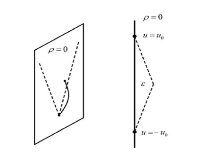
Figure 1: The time-like trajectory in the bulk by following kelly_14 .

The bulk causality gives an inequality with a bound,

$$\frac{2}{u_{0}}\int_{-u_{0}}^{u_{0}}du\left(\frac{u_{0}-|u|}{u_{0}}\right)^{3}\left(\langle T_{ab}(u,0)\rangle K^{a}K^{b}\right)\geq-\frac{3\,N^{2}}{2\pi L^{3}}\frac{1}{u_{0}^{5/4}}\,$$ (59)

that is consistent with kelly_14 . All detailed proof will be described in Appendix. In the $u_{0}\rightarrow\infty$ ($\varepsilon\rightarrow 0$) limit, since the path in the boundary becomes null-like, we can identify $u=\frac{\sqrt{2}}{L}\lambda$, where $\lambda$ is an affine parameter along the null geodesic. The stress tensor is found to satisfy the average null energy condition as:

$$\lim_{\lambda_{0}\rightarrow\infty}\,\int d\lambda\,g_{\lambda_{0}}(\lambda)\,\left(\langle T_{ab}(\lambda)\rangle K^{a}K^{b}\right)\geq 0\,$$ (60)

with the sampling function $g_{\lambda_{0}}(\lambda)$ (54). Thus, we have a general proof of the null energy condition for the holographic stress tensor in $z=1$ case as the sampling function is chosen in (54).

Nevertheless the above lower bound for a finite $\lambda_{0}$ is not invariant under rescaling of an affine parameter that may not be meaningful. In free relativistic field theory, such lower bound for null-like geodesics does not exist either, except in $1+1$ dimensions as will be seen later.

Therefore we come to find a possible quantum inequality by evaluating the null-contracted energy density along some other path rather than a null geodesic. In FE_03 , the null-contracted energy density along the time-like path is considered. Such a transverse smearing wald gives a lower bound on the null energy density. To do so, in the holographic framework, we evaluate $t_{uu}$ along a time-like path in the boundary by setting $v=-\overline{v}(u)$ in (VI) (also see Appendix for details). Thus, the quantum inequality is achieved in terms of $v=-\overline{v}(u)$ with a bound,

$$\frac{2}{u_{0}}\int_{-u_{0}}^{u_{0}}du\left(\frac{u_{0}-|u|}{u_{0}}\right)^{3}\left(\langle T_{ab}(u,-\overline{v}(u))\rangle K^{a}K^{b}\right)\geq-\frac{3\,N^{2}}{2\pi L^{3}}\frac{1}{u_{0}^{3/2}}\,.$$ (61)

The prescribed time-like path has velocity $V\simeq 1+\frac{d\overline{v}(u)}{du}\simeq 1-u_{0}^{-3/2}$. In particular, for a large value of $u_{0}$, the path is close to the null trajectory with Lorentz factor $\gamma\simeq(\tau_{0}/L)^{3}\gg 1$ where a proper time $\tau_{0}\simeq\gamma^{-1}u_{0}\simeq Lu_{0}^{1/4}$. The bound can be expressed in a Lorentz invariant form:

$$\int d\tau\,g_{\tau_{0}}(\tau)\,\left(\langle T_{ab}(\tau)\rangle K^{a}K^{b}\right)\gtrsim-\frac{3\,N^{2}}{2\pi L^{3}}\frac{L^{6}}{\tau_{0}^{6}}\,,$$ (62)

that is now a function of the proper time with the smearing function $g_{(\tau_{0})}(\tau)$ given in (54). Again, as $\tau_{0}\rightarrow\infty$, the above inequality leads to the averaged energy condition. Notice that since $V^{a}=(\gamma,0,-\gamma V)$ and $K^{a}=(1,0,-1)$, $(V_{a}K^{a})^{2}\simeq\gamma^{2}\simeq L^{6}/\tau_{0}^{6}$ for a large $\gamma$ factor. Thus the right hand side of the bound can be written in the form $(V_{a}K^{a})^{2}$ of manifest invariance under the rescaling of an affine parameter. This inequality (62) is one of the main results in this work. Notice that the above inequality is achieved by explicitly constructing a particular path. From the boundary point of view Visser_09 , we may regard $L$ as a characteristic length scaling of quantum critical theories. The $1/L^{3}$ dependence in (62) gives correct units for energy density in 2+1-dimensional spacetime. Later we will compare with similar inequality obtained from free relativistic field theory in that the expected dependence with units of energy density is characterized by $1/\tau_{0}^{3}$. For $\tau_{0}>L$, the inequality from strongly coupled field will give a weaker constraint on negative null energy density as compared with the constraint from the free relativistic field when they both have same value of $(K^{a}V_{a})^{2}$.

To see the consequence of the negative lower bound, we will derive the constraint on the duration of null negative energy. The averaged stress tensor over a time-like path can be found from (52) and (53) in that the affine parameter is replaced by a proper time, $\lambda\rightarrow\gamma\tau$ in the case of $z=1$. We can see that, within the initial time $\Delta\tau=\sqrt{2\sigma}/\gamma$, the null energy density is dominated by the piece of negative energy density with its magnitude in a spatial region $\Omega_{2}$ to be

$$\frac{|\Delta E|}{\Omega_{2}}=\frac{|\alpha|N^{2}}{128\sqrt{\pi}\,\,\sigma^{3/2}}\,.$$ (63)

With the result (IV.1) by letting $\lambda=\gamma\tau_{0}$ and $z=1$, the bound (62) gives an inequality as

$$\frac{N^{2}}{\sigma^{3/2}}\left(\frac{3|\alpha|^{2}}{256\sqrt{2}\sqrt{\pi}}-\frac{3|\alpha|}{64\sqrt{\pi}}\frac{\sigma}{\gamma^{2}\,\tau_{0}^{2}}\right)\gtrsim-\frac{3\,N^{2}}{2\pi L^{3}}\frac{L^{6}}{\tau_{0}^{6}}\,.$$ (64)

Within the above $\Delta\tau$, the most stringent bound imposed on negative energy density can be obtained by ignoring its positive contribution and letting $\sigma=\tau_{0}^{2}\gamma^{2}|\alpha|$, giving

$$\frac{|\Delta E|}{\Omega_{2}}(\Delta\tau)^{3}\leq\frac{N^{2}}{\sqrt{2}\pi}\sqrt{|\alpha|}\,\frac{L^{3}}{\tau_{0}^{3}}\,.$$ (65)

Again, the above bound is valid for $\tau_{0}\gg L$ from the holographic construction. Recall that the above quantum inequality is for the time-like trajectory with velocity

$$V=1-\frac{1}{(\tau_{0}/L)^{6}}\,,$$ (66)

which means that the bound is valid only for the geodesic path very close to be null. Later we will make a comparison with the quantum inequality from free relativistic field theory with the same $V$, where a more restricted condition on negative energy is expected.

IV.2 free field theory

We now turn to considering the average null energy condition for conformally coupled free massless scalar fields in $2+1$ dimensional Minkowski spacetime for a comparison. We choose the small squeezing parameter $F$ in (50). With the same null tangent vector $K_{a}=(1,0,-1)$ as above and the sampling function (54), the averaged null energy for the stress tensor over an affine parameter, which can be obtained from (46) by letting $\lambda=t$, up to the second order in small $F$, becomes

$$\int\,g_{\lambda_{0}}(\lambda)\,\langle T_{ab}(\lambda)\rangle_{R}K^{a}K^{b}\,d\lambda=\frac{2}{\lambda_{0}}\int_{-\lambda_{0}}^{\lambda_{0}}d\lambda\left(\frac{\lambda_{0}-|\lambda|}{\lambda_{0}}\right)^{3}\left(\langle T_{00}\rangle_{R}+\langle T_{22}\rangle_{R}\right)(\lambda)$$

$$\quad\quad\quad\quad\quad\quad\quad\quad\quad\quad\quad\quad\quad\quad\quad\quad=\frac{9\,|\alpha|^{2}N^{2}}{1016\sqrt{\pi}}\sigma^{-\frac{3}{2}}-\frac{3\,|\alpha|N^{2}}{64\sqrt{\pi}}\sigma^{-\frac{3}{2}}\frac{\sigma}{\lambda_{0}^{2}}\,.$$ (67)

We then find the associated quantum inequality, if exists. The explicit expressions for the relevant $T_{ab}$ are given by (42),

$$T_{00} = N^{2}\bigg{(}\frac{3}{4}\dot{\psi}^{2}(x)-\frac{1}{4}\big{(}\dot{\psi}^{2}(x)-(\nabla\psi(x))^{2}\big{)}-\frac{1}{4}\psi(x)\ddot{\psi}(x)-\frac{1}{36}\psi(x)\partial^{2}\psi(x)\bigg{)}\,,$$

$$T_{ii} = N^{2}\bigg{(}\frac{3}{4}(\partial_{i}{\psi}(x))^{2}+\frac{1}{4}\big{(}\dot{\psi}^{2}(x)-(\nabla\psi(x))^{2}\big{)}-\frac{1}{4}\psi(x)\partial_{i}^{2}\psi(x)+\frac{1}{36}\psi(x)\partial^{2}\psi(x)\bigg{)}\,,$$

$$T_{0i} = N^{2}\bigg{(}\frac{2}{3}\dot{\psi}\partial_{i}\psi-\frac{1}{3}\psi\partial_{i}\dot{\psi}\bigg{)}\,.$$ (68)

For the purpose of showing potential divergence in deriving quantum inequalities, let us consider the trajectory $x^{a}_{\epsilon}=\lambda(1,0,-{\mathrm{v}})$, where ${\mathrm{v}}=1-\epsilon$, and in the limit $\epsilon\rightarrow 0^{+}$ the trajectory is along the null geodesic. The mode functions (44) evaluated along this nearly null geodesic are

$$f_{{\bf k},{\mathrm{v}}}(x)=e^{-i(k+{\mathrm{v}}k_{2})\lambda}\,.$$ (69)

Now the mode functions are smeared by the sampling function $g_{\lambda_{0}}(\lambda)$ in (54), and become:

$$h^{\pm}_{{\bf k}{\mathrm{v}}} \equiv h_{{\bf k}{\mathrm{v}}}=\frac{2}{\lambda_{0}}\int_{-\lambda_{0}}^{\lambda_{0}}\,d\lambda\,\Bigg{(}\frac{\lambda_{0}-|\lambda|}{\lambda_{0}}\Bigg{)}^{3}\frac{e^{\pm i(k+{\mathrm{v}}k_{2})\lambda}}{\sqrt{2k}}$$ (70)

$$= -\sqrt{\frac{2}{k}}\frac{1}{(k+{\mathrm{v}}k_{2})^{4}\lambda_{0}^{4}}\,\Big{[}12-12\,\cos[(k+{\mathrm{v}}k_{2})\lambda_{0}]-6(k+{\mathrm{v}}k_{2})^{2}\lambda_{0}^{2}\Big{]}\,.$$

The dot means the derivative with respect to time $t$. After taking integration by parts and dropping out irrelevant total derivative terms, the null contracted stress tensor, $T_{ab}K^{a}K^{b}=T_{00}-T_{02}-T_{20}+T_{22}$, can be cast into the form of the product of the operator and its hermitian conjugate. Thus, its expectation value is positive definite as below:

$$\int d\lambda\,g_{\lambda_{0}}(\lambda)\langle T_{00}-T_{02}-T_{20}+T_{22}\rangle(\lambda)=N^{2}\int\frac{d^{2}{\bf k}}{(2\pi)^{2}}\,\frac{d^{2}{\bf k^{\prime}}}{((2\pi)^{2}}(k+k_{2})(k^{\prime}+k^{\prime}_{2})\,h_{{\bf k}{\mathrm{v}}}h_{{\bf k^{\prime}}{\mathrm{v}}}$$

$$\quad\quad\quad\quad\quad\quad\quad\times\bigg{[}-\langle a_{\bf k}\,a_{\bf k^{\prime}}+\langle a_{\bf k}\,a^{\dagger}_{\bf k^{\prime}}\rangle\,+\langle a^{\dagger}_{\bf k}\,a_{\bf k^{\prime}}\rangle\,-\langle a^{\dagger}_{\bf k}\,a^{\dagger}_{\bf k^{\prime}}\rangle\,\bigg{]}\geq 0\,.$$ (71)

As such, the renormalized $\langle T_{ab}\rangle K^{a}K^{b}$ by normal-ordering is found to have a lower bound,

$$\int d\lambda\,g_{\lambda_{0}}(\lambda)\langle T_{ab}(\lambda)\rangle_{R}K^{a}K^{b} \geq-N^{2}\int\frac{d^{2}{\bf k}}{(2\pi)^{2}}\,\frac{d^{2}{\bf k^{\prime}}}{((2\pi)^{2}}(k+k_{2})(k^{\prime}+k^{\prime}_{2})\,h_{{\bf k}{\mathrm{v}}}h_{{\bf k^{\prime}}{\mathrm{v}}}$$ (72)

$$\quad\quad\quad\quad\quad\quad\quad\times\bigg{[}\left(\langle a_{\bf k^{\prime}}\,a^{\dagger}_{\bf k}\rangle-\langle a^{\dagger}_{\bf k}\,a_{\bf k^{\prime}}\rangle\right)\bigg{]}$$

$$=-N^{2}\int\frac{d^{2}{\bf k}}{(2\pi)^{2}}(k+k_{2})^{2}\,h_{{\bf k}{\mathrm{v}}}^{2}\,=-N^{2}\,\frac{27}{5}\,\frac{1}{\lambda_{0}^{3}\,(1+{\mathrm{v}}^{2})\,\sqrt{1-{\mathrm{v}}^{2}}}\,$$

$$\simeq-N^{2}\,\frac{27}{10}\,\frac{1}{\lambda_{0}^{3}\epsilon}$$

The integral diverges in the light-cone limit $\epsilon\rightarrow 0^{+}$. Thus, for a finite $\lambda_{0}$, there is no lower bound for free relativistic field theory. This is consistent with the findings in FE_03 .

According to FE_03 , an alternative way to obtain quantum inequalities is to consider the null-contracted stress tensor in a rest frame of the time-like trajectory described by a proper time $\tau$. In this frame, the negative lower bound for the average null energy is obtained from (72) by setting ${\mathrm{v}}=0$ and replacing $\lambda_{0}\rightarrow\tau_{0}$. Then it can be written in the form that is invariant under the rescaling of an affine parameter,

$$\int d\lambda\,g_{\tau_{0}}(\tau)\langle T_{ab}(\tau)\rangle_{R}K^{a}K^{b}\geq-N^{2}\,\frac{27}{5}\,\frac{(K^{a}V_{a})^{2}}{\tau_{0}^{3}}\,,$$ (73)

where $V^{a}$ is a velocity vector of the time-like trajectory. To compare with the quantum inequality for strongly coupled fields in (62), we substitute $V^{a}$ with velocity (66), namely $(K^{a}V_{a})^{2}\approx(\tau_{0}/L)^{6}$, into above result. For $\tau_{0}\gg L$, it seems to indicate that the quantum inequality for strongly coupled fields gives weaker constraint than the one for free relativistic fields.

To find the constraint on the negative null energy, we choose the small squeezing parameter $F$ as in (50) and following the procedure above, the magnitude of the negative null energy within the duration time $\Delta\tau$ obeys an inequality,

$$\frac{|\Delta E|}{\Omega_{2}}(\Delta\tau)^{3}<\frac{9N^{2}}{5\sqrt{2}}\sqrt{|\alpha|}\,(K^{a}V_{a})^{2}\,,$$ (74)

where $(K^{a}V_{a})^{2}\simeq(L/\tau_{0})^{6}\ll 1$. Thus, as compared with (65), we find that in strongly coupled field theory larger $\Delta\tau$ is allowed for a fixed $|\Delta E|$. Whether or not the above feature is also true for other quantum states with negative energy density needs the further study.

V Conclusion

In this paper, we have used the AdS/CFT correspondence to study the expectation value of stress tensor in $2+1$-dimensional strongly coupled quantum critical theories with Lifshitz scaling symmetry. The holographic dual theory is the gravity theory in 3+1-dimensional Lifshitz geometry. We adopt the consistent scheme to construct the boundary stress tensor that satisfies the trace Ward identity due to Lifshitz scaling symmetry. The boundary stress tensor, obtained from the gravitational wave deformed Lifshitz geometry, can be found up to second order in gravitational wave perturbations, and is compared to its counterpart for free scalar fields at same order in an expansion of small squeezing parameters. We can then relate the boundary values of gravitational waves to the squeezing parameters of squeezed vacuum states. We find that, in both cases with $z=1$, the leading order term of stress tensor for a small squeezing parameter reveals oscillation between negative and positive values in time and settles to zero at late times. This piece can be identified with the principal based upon the quantum interest conjecture in Ford_99 . The subleading term is spacetime uniform with a positive constant value, and can be identified with the interest. The averaged null energy condition along the null trajectory with an affine parameter $\lambda_{0}$ is studied in the $z=1$ case. We find that, although the sum of the leading and subleading terms in a small squeezing parameter expansion may be negative for small $\lambda_{0}$, the averaged null energy density then becomes positive in the limit of $\lambda_{0}\rightarrow\infty$, which satisfies the averaged null energy condition, and is thus consistent with the quantum interest conjecture Ford_99 .

We then try to find the associated negative lower bound to the averaged null-contracted stress tensor, also for the case of $z=1$. For the average over the complete null geodesic, the bound exists for quantum critical fields while there is no such bound for free relativistic fields. An alternative smearing is introduced, in that the null-contracted stress tensor is averaged over time-like trajectories. For the trajectories along nearly null directions, the bounds are found. We find the weaker constraint on the magnitude and duration of negative null energy density in strongly coupled field theories as compared with the constraint in free relativistic field theories. Thus, it implies that the negative energy density for strongly coupled fields might be allowed to last longer, before the overcompensation from the piece of positive energy density, than for weakly coupled fields. This might give some implications to the existence of exotic spacetimes sourced by quantum fields with negative energy density. Whether or not this feature remains true in more general time-like trajectories, spacetime dimensions and other quantum states deserves future study.

VI Appendix

In this Appendix, we will present the detailed description on how the inequalities (59) and (61) are obtained. In the $z=1$ case, the background is just the 3+1-dimensional AdS space and the metric can be rewritten from (4) as

$$ds^{2}=\frac{L^{2}}{\rho^{2}}(d\rho^{2}-dudv-dvdu+dy^{2})\,$$ (75)

with the chosen coordinates $\rho=\frac{L}{r}$, $u=\frac{1}{\sqrt{2}L}(t+x_{2})$, $v=\frac{1}{\sqrt{2}L}(t-x_{2})$ and $x_{1}=\frac{y}{L}$. Then, the perturbed metric can be parameterized as

$$\frac{L^{2}}{\rho^{2}}\big{(}d\rho^{2}-dudv-dvdu+dy^{2}+\rho^{3}(t_{uu}du^{2}+t_{vv}dv^{2}+t_{uv}dudv+t_{yy}dy^{2})\big{)}\,.$$ (76)

In the limit of $r\rightarrow\infty$ ($\rho\rightarrow 0$) and using the identification (21), we can write

$$t_{uu}=\frac{8\pi G_{4}L}{3}\,\langle T_{ab}\rangle_{R}K^{a}K^{b}+\mathcal{O}(\rho^{2})\,,$$ (77)

where $K^{a}=(1,0,-1)$ is described above. Other components of metric perturbations can have the similar expansion, but here we will particularly focus on the $t_{uu}$ component. We now construct a causal (time-like) trajectory in the bulk shown in Fig.1 given by

$$\bar{\rho}(u)=\varepsilon\left(\frac{u_{0}-|u|}{u_{0}}\right)\,,$$

$$\bar{v}(u)=\frac{\varepsilon^{2-\Delta}}{2u_{0}}\left(\frac{u_{0}+u}{u_{0}}\right)+\frac{\varepsilon^{3}}{2}\int_{-u_{0}}^{u}du^{\prime}\left(\frac{u_{0}-|u^{\prime}|}{u_{0}}\right)^{3}t_{uu}(u^{\prime},v(u^{\prime}))$$ (78)

for $-u_{0}\leq u\leq u_{0}$ and $\Delta>0$. In addition, $u=\pm u_{0}$ are on the boundary. We require $\varepsilon$ to be small so the path is close to the boundary, and $u_{0}$ to be large for having an interesting bound. The (bulk) time-like condition $g_{\mu\nu}\frac{dx^{\mu}}{du}\frac{dx^{\nu}}{du}\leq 0$ gives

$$(\bar{\rho}^{\prime})^{2}-2\bar{v}^{\prime}+\bar{\rho}^{3}\left(t_{uu}+t_{uv}\bar{v}^{\prime}+t_{vv}\bar{v}^{\prime 2}\right)\leq 0\,.$$ (79)

The prime here denotes the derivative with respect to $u$. With the prescribed path, the bulk causality above is satisfied if

$$\frac{\varepsilon^{2-\Delta}}{u_{0}^{2}}>\mathcal{O}(\varepsilon^{6})\,.$$ (80)

Having described the causal trajectory (VI), the theorem in Wald_00 shows that the end point located at the boundary $\rho=0$ must be also causally separated,

$$\bar{v}(u_{0})-\bar{v}(-u_{0})=\frac{\varepsilon^{3}}{2}\int_{-u_{0}}^{u_{0}}du^{\prime}\left(\frac{u_{0}-|u^{\prime}|}{u_{0}}\right)^{3}t_{uu}+\frac{\varepsilon^{2-\Delta}}{u_{0}}\geq 0\,,$$ (81)

leading to the quantum inequality for the null energy density. Along the trajectory (VI), the value of the coordinate $v$ is small, and $t_{uu}$ can be expanded in terms of small $v$. Thus the inequality (81) gives,

$$\frac{2}{u_{0}}\int_{-u_{0}}^{u_{0}}du^{\prime}\left(\frac{u_{0}-|u^{\prime}|}{u_{0}}\right)^{3}\left(t_{uu}(u^{\prime},0)+\partial_{v}t_{uu}(u^{\prime},0)\bar{v}(u^{\prime})+...\right)\geq-\frac{4\varepsilon^{-1-\Delta}}{u_{0}^{2}}\,.$$ (82)

Assuming that the integral over energy-momentum tensor and all its derivatives are all finite kelly_14 , we may ignore the sub-leading terms if

$$\frac{\varepsilon^{-1-\Delta}}{u_{0}^{2}}>\mathcal{O}(\bar{v})\,.$$ (83)

Then the inequality (82) becomes

$$\frac{2}{u_{0}}\int_{-u_{0}}^{u_{0}}du^{\prime}\left(\frac{u_{0}-|u^{\prime}|}{u_{0}}\right)^{3}t_{uu}(u^{\prime},0)\geq-\frac{4\varepsilon^{-1-\Delta}}{u_{0}^{2}}\,.$$ (84)

To satisfy (80) and (83), we find that the most stringent bound is obtained when considering $\mathcal{O}(\bar{v})\sim\varepsilon^{3}u_{0}$, and letting $\Delta\rightarrow 0$ and $u_{0}\rightarrow\varepsilon^{-4/3}$. The inequality (59) is obtained. Note that in finding quantum inequalities, we ignore the order $\rho^{2}$ terms in (77) in the form of $\rho^{2}s_{uu}$ where $s_{uu}$ is the algebraic function of the renormalized expectation value of stress tensor and its derivatives kelly_14 . Nevertheless for a bounded renormalized expectation value of stress tensor such as the one in (52), and (53), the smeared $t_{ab}$ over $u$ is in general independent of $u_{0}$ or inversely proportional to the powers of $u_{0}$. The corrections from the ignored terms, when letting $u_{0}\rightarrow\varepsilon^{-4/3}$, are at most of order $\varepsilon^{2}$, which give ignorable contributions as compared with the lower bound in the right hand side of (84) in the limit of $\varepsilon\rightarrow 0$.

As for the average over the time-like path, we evaluate $t_{uu}$ along a path in the boundary by setting $v=-\overline{v}(u)$ in (82). Then, in this case the most stringent bound which is solely due to (80), is by setting $\Delta\rightarrow 0$ and $u_{0}\rightarrow\varepsilon^{-2}$ to achieve (61).

- (1) R. Penrose, ”Gravitational collapse and space-time singularities”, Phys. Rev. Lett. 14, (1965) 57 (1965); S. Hawking, ”The Occurrence of singularities in cosmology”, Proc. Roy. Soc. Lond. A 294, 511 (1966); S. Hawking and R. Penrose, ”The Singularities of gravitational collapse and cosmology”, Proc. Roy. Soc. Lond. A 314, 529 (1970).
- (2) H. Epstein, V. Glaser, and A. Jaffe, ”Nonpositivity of energy density in quantized field theories”, Nuovo Cimento 36, 1016 (1965).
- (3) L. H. Ford, ”Quantum coherence effects and the second law of thermodynamics”, Proc. R. Soc. London A 346, 227 (1978).
- (4) P. C. W. Davies, Phys. Lett. B 113, 393 (1982).
- (5) L. H. Ford and T. A. Roman, Phys. Rev. D 41, 3662 (1990) ; L. H. Ford and T. A. Roman, Phys. Rev. D 46, 1328 (1992).
- (6) M. S. Morris and K. S. Thorne, Am. J. Phys. 56, 395 (1988); M. S. Morris, K. S. Thorne, and U. Yurtsever, Phys. Rev. Lett. 61, 1446 (1988).
- (7) M. Alcubierre, ”The Warp drive: hyperfast travel within general relativity”, Class. Quantum Grav. 11, L-73 (1994).
- (8) L. Ford and T. A. Roman, ”Quantum field theory constraints traversable wormhole geometries”, Phys. Rev. D 53, 5496 (1996), arXiv:gr-qc/9510071.
- (9) D. Hochberg and M. Visser, ”The null energy condition in dynamic wormholes”, Phys. Rev. Lett. 81, 746 (1998), arXiv:gr-qc/9802048; M. Visser, S. Kar, and N. Dadhich, ”Traversable wormholes with arbitrarily small energy condition violations”, Phys. Rev. Lett. 90, 201102 (2003), arXiv:gr-qc/0301003.
- (10) A. Ori, ”Must time machine construction violate the weak energy condition?”, Phys. Rev. Lett. 71, 2517 (1993).
- (11) R. Myrzakulov, L. Sebastiani, S. Vagnozzi, and S. Zerbini, ”Static spherically symmetric solutions in mimetic gravity: rotation curves and wormholes”, Class. Quantum Grav. 33, 125005 (2016), arXiv:gr-qc/1510.02284.
- (12) L. H. Ford, ”Constraints on negative-energy fluxes”, Phys. Rev. D 43, 3972 (1991).
- (13) L. H. Ford and Thomas A. Roman, ” Averaged energy conditions and quantum inequalities”, Phys. Rev. D 51, 4277 (1995).
- (14) M. J. Pfenning and L. H. Ford, Phys. Rev. D 57, 3489 (1998); L. H. Ford, M. J. Pfenning, and T. A. Roman, Phys. Rev. D 57, 4839 (1998).
- (15) C. Fewster and S. Eveson, Phys. Rev. D 58, 084010 (1998).
- (16) C. J. Fewster and T. A. Roman, ”Null energy conditions in quantum field theory”, Phys. Rev. D 67, 044003 (2003).
- (17) L. Ford, T. Roman, “The quantum interest conjecture”, Phys. Rev. D 60, 104018 (1999), arXiv:gr-qc/9901074.
- (18) J.-T. Hsiang, T.-H. Wu, and D.-S, Lee, Phys. Rev. D 77, 105021 (2008).
- (19) J.-T. Hsiang, T.-H. Wu, and D.-S. Lee, Ann. Phys. 327, 522 (2012).
- (20) J.-T. Hsiang and L. H. Ford, Phys. Rev. Lett. 92, 250402 (2004).
- (21) J.-T. Hsiang and D.-S. Lee, Phys. Rev. D 73, 065022 (2006).
- (22) J. M. Maldacena, Adv. Theor. Math. Phys. 2, 231 (1998) (Int. J. Theor. Phys. 38, 1113 (1999)); S. S. Gubser, I. R. Klebanov and A. M. Polyakov, Phys. Lett. B 428, 105 (1998); E. Witten, Adv. Theor. Math. Phys. 2, 253 (1998).
- (23) C. P. Herzog, A. Karch, P. Kovtun, C. Kozcaz, and L. G. Yaffe, “Energy loss of a heavy quark moving through supersymmetric Yang-Mills plasma”, JHEP 07, 013 (2006).
- (24) S. S. Gubser, “Drag force in AdS/CFT”, Phys. Rev. D 74, 126005 (2006).
- (25) J. Casalderrey-Solana and D. Teaney, “Heavy quark diffusion in strongly coupled Yang-Mills theory”, Phys. Rev. D 74, 085012 (2006).
- (26) D. T. Son and D. Teaney,“Thermal noise and stochastic strings in AdS/CFT”, JHEP 07, 021 (2009).
- (27) G. C. Giecold, E. Iancu, and A. H. Mueller,“Stochastic trailing string and Langevin dynamics from AdS/CFT”, JHEP 07, 033 (2009).
- (28) J. Casalderrey-Solana, K.-Y. Kim, and D. Teaney,“Stochastic string motion above and below the world sheet horizon”, JHEP 12, 066 (2009).
- (29) S. Caron-Huot, P. Chesler and D. Teaney, “Fluctuation, dissipation and thermalization in non-equilibrium black hole geometries”, Phys. Rev. D 84, 026012 (2012).
- (30) J. Boer, V. Hubeny, M. Rangamani and M. Shigemori, “Brownian motion in AdS/CFT”, JHEP 07, 094 (2009); V. Hubeny and M. Rangamani,“A holographic view on physics out of equilibrium”, Adv. High Energy Phys. 2010, 297916 (2010).
- (31) D. Tong and K. Wong, “Fluctuation and dissipation at a quantum critical point”, Phys. Rev. Lett. 110, 061602 (2013).
- (32) C.-P. Yeh, J.-T. Hsiang, D.-S. Lee, ”Holographic approach to nonequilibrium dynamics of moving mirrors coupled to quantum critical theories”, Phys. Rev. D 89, 066007 (2014).
- (33) C.-P. Yeh, J.-T. Hsiang, D.-S. Lee,” Holographic influence functional and its application to decoherence induced by quantum critical theories”, Phys. Rev. D 91, 046009 (2015).
- (34) C.-P. Yeh, D.-S. Lee, ”Subvacuum effects in quantum critical theories from holographic approach”, Phys. Rev. D 93, 126006 (2016). arXiv:1410.7111.
- (35) R. Bousso, Z. Fisher, J. Koeller, S. Leichenauer, and A. C. Wall, “Proof of the quantum null energy condition“, Phys. Rev. D 93, 024017 (2016), arXiv:gr-qc/1509.02542.
- (36) J. Koeller, S. Leichenauer, “Holographic proof of the quantum null energy condition“, arXiv:gr-qc/1512.06109.
- (37) W. R. Kelly and A. C. Wall, “A holographic proof of the averaged null energy condition”, Phys. Rev. D 91, 069902 (2015), arXiv:gr-qc/1408.3566; Erratum: Holographic proof of the averaged null energy condition [Phys. Rev. D 90, 106003 (2014)], Phys. Rev. D 91, 069902(E) (2015).
- (38) J. Polchinski, L. Susskind and N. Toumbas, “Negative energy, superluminosity and holography”, Phys. Rev. D 60, 084006 (1999), arXiv:hep-th/9903228.
- (39) S. Kachru, X. Liu and M. Mulligan, “Gravity duals of Lifshitz-like fixed points”, Phys. Rev. D 78, 106005 (2008).
- (40) M. Taylor, “Non-relativistic holography”, arXiv:hep-th/0812.0530; ”Lifshitz holography”, arXiv:hep-th/1512.03554.
- (41) V. Balasubramanian and P. Kraus, “A stress tensor for anti-de Sitter gravity”, Commun. Math. Phys. 208, (1999) 413-428 (1999), arXiv:hep-th/9902121.
- (42) R. Myers, “Stress tensors and casimir energies in the AdS/CFT corresponsce”, Phys. Rev. D 60, 046002 (1999), arXiv:hep-th/9903203.
- (43) S. Hollands, A. Ishibashi and D. Marolf, “Counter-term charges generate bulk symmetries”, Phys. Rev. D 72, 104025 (2005), arXiv:hep-th/0503105.
- (44) S. Ross and O. Saremi, “Holographic stress tensor for non-relativistic theories”, JHEP 09, 009 (2009), arXiv:hep-th/0907.1846.
- (45) K. Schleich and D. Witt, “A simple proof of Birkhoff’s theorem for cosmological constant”, J. Math. Phys. 51, 112502 (2010), arXiv:gr-qc/0908.4110.
- (46) E. Brynjolfsson, U. Danielsson, L. Thorlacius and T. Zingg, “Holographic superconductors with Lifshitz scaling”, J. Phys. A: Math. Theor. 43, 065401 (2010), arXiv:hep-th/0908.2611.
- (47) K. Bronnikov and M. Kovalchuk, “On a generalisation of Birkhoff s theorem ”, J. Phys. A: Math. Gen. 13, 187 (1980).
- (48) G. Bertoldi, B. Burrington and A. Peet, “Thermodynamics of black branes in asymptotically Lifshitz spacetimes ”, Phys. Rev. D 80, 126004 (2009), arXiv:hep-th/0907.4755.
- (49) N. D. Birrell, P. C. W. Davies, Quantum Fields in Curved Space (Cambridge University Press).
- (50) E. Flanagan and R. M. Wald, Phys. Rev. D 54, 6233 (1996).
- (51) M. Visser, Phys. Rev. D 80, 025011 (2009), arXiv:hep-th/0902.0590.
- (52) S. Gao and R. M. Wald, “Theorems on gravitational time delay and related issues”, Class. Quant. Grav. 17, 4999 (2000), arXiv:gr-qc/0007021.