The Galactic Nova Rate Revisited

Abstract

Despite its fundamental importance, a reliable estimate of the Galactic nova rate has remained elusive. Here, the overall Galactic nova rate is estimated by extrapolating the observed rate for novae reaching $m\leq 2$ to include the entire Galaxy using a two component disk plus bulge model for the distribution of stars in the Milky Way. The present analysis improves on previous work by considering important corrections for incompleteness in the observed rate of bright novae and by employing a Monte Carlo analysis to better estimate the uncertainty in the derived nova rates. Several models are considered to account for differences in the assumed properties of bulge and disk nova populations and in the absolute magnitude distribution. The simplest models, which assume uniform properties between bulge and disk novae, predict Galactic nova rates of $\sim$50 to in excess of 100 per year, depending on the assumed incompleteness at bright magnitudes. Models where the disk novae are assumed to be more luminous than bulge novae are explored, and predict nova rates up to 30% lower, in the range of $\sim$35 to $\sim$75 per year. An average of the most plausible models yields a rate of $50_{-23}^{+31}$ yr^-1, which is arguably the best estimate currently available for the nova rate in the Galaxy. Virtually all models produce rates that represent significant increases over recent estimates, and bring the Galactic nova rate into better agreement with that expected based on comparison with the latest results from extragalactic surveys.

1. Introduction

The Galactic nova rate is important in the study of a variety of astrophysical problems. For example, classical nova explosions are thought to play a significant role in the chemical evolution of the Galaxy (e.g., José et al., 2006, and references therein). In addition to producing a fraction of the ⁷Li and the short-lived isotopes ²²Na and ²⁶Al, novae are believed to be important in the production of the CNO isotopes, particularly ¹⁵N, where novae may account for virtually all of the Galactic abundance of this isotope. Thus, complete models for Galactic chemical evolution necessarily require the nova rate as an input parameter.

Novae may also play an important role as Type Ia supernova (SN Ia) progenitors (Shafter et al., 2015; Soraisam & Gilfanov, 2015; Starrfield et al., 2016, and references therein). Indeed, perhaps the most promising SN Ia progenitor extant is the recurrent nova, M31N 2008-12a (Henze et al., 2015a; Tang et al., 2014; Darnley et al., 2015). M31N 2008-12a has an extremely short recurrence time of just under a year, possibly as short as 6 months (Henze et al., 2015b), which constrains the accretion rate to be $2-3\times 10^{-7}$ M_⊙ yr^-1 and the mass of the white dwarf to be near the Chandrasekhar limit (Kato et al., 2014; Wolf et al., 2013). These models also suggest that the white dwarf is gaining mass, and that it will reach the Chandrasekhar limit in less than $10^{6}$ years. The ultimate fate of M31N 2008-12a, as with all similar recurrent nova systems, depends on whether the composition of the white dwarf is CO or ONe. In the former case the system is expected to explode as a SN Ia, while in the latter case electron captures onto ²⁰Ne and ²⁴Mg will result in an accretion-induced collapse and the subsequent formation of a neutron star (Miyaji et al., 1980).

Despite its importance, the Galactic nova rate is not well established. Estimates have varied widely, from as few as 20 to as many as 260 yr^-1 (della Valle & Livio, 1994; Sharov, 1972). Recently, Mróz et al. (2015) have measured a rate of $13.8\pm 2.6$ yr^-1 for the Galactic bulge alone based on OGLE observations. Global nova rates have been estimated both directly, by extrapolating the observed rate in the vicinity of the sun to the entire Galaxy (e.g., see Shafter, 1997, 2002), and indirectly through comparison with other galaxies (Shafter et. al., 2000; Darnley et al., 2006; Shafter et al., 2014). Shafter (2002) used the Bahcall & Soneira (1980) model for the stellar density in the Milky Way to extrapolate the rate of novae with $m\mathrel{\hbox{\hbox to0.0pt{\hbox{\lower 4.0pt\hbox{$\sim$}}\hss}\hbox{$<$}}}2$, which was assumed to be complete, to faint magnitudes finding a Galactic rate of $36\pm 13$ yr^-1. Recently, Schaefer (2014) performed a thorough analysis of the observational selection biases against the discovery of even the brightest novae. After taking these biases into account, Schaefer (2014) makes the surprising suggestion that only $43\pm 6$% of Galactic novae with $m\leq 2$ are likely recovered.

In this paper, we reconsider the analysis presented in Shafter (2002) and Shafter (1997) by conducting Monte Carlo simulations to estimate the global Galactic nova rate and its uncertainty. The revised analysis includes the increased sample of Galactic novae available since 2000, and makes more plausible assumptions regarding the completeness of the nova sample at bright magnitudes. We conclude by comparing the latest Galactic nova estimates with those recently measured in extragalactic systems such as the nearby spiral M31, and the Virgo elliptical M87.

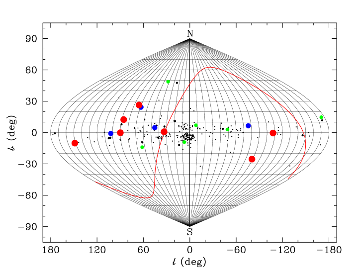
Figure 1.— The distribution of Galactic novae brighter than $m=10$ discovered since 1900 are displayed in Galactic coordinates. Key – red filled circles: $m\leq 2$, smaller blue filled circles: $m\leq 3$, smaller green filled circles: $m\leq 4$, smaller black filled circles: $m\leq 5$, smallest black dots: $m\leq 10$. The solid red line represents the Celestial equator. Note the large concentration of faint novae toward the Galactic center and the apparent bias for brighter novae in the Northern hemisphere.

2. The Observed Nova Sample

From 1900 to the end of 2015 there have been a total of $\sim$250 Galactic novae discovered brighter than $m=10$, and we have compiled a list of these novae in Table 1. The spatial positions of the full nova sample from Table 1 are plotted in Figure 1, which confirms that the novae are concentrated in the Galactic plane, and in the direction of the Galactic center. The observed asymmetry about Galactic latitude $b=0$ confirms the presence of significant and patchy absorption in the disk plane. Clearly, magnitude-limited samples of novae will be incomplete, particularly at fainter magnitudes.

Table 1Galactic Novae Since 1900

Nova	Name	Date (Y,M,D)	$l$ (∘)	$b$ (∘)	$m_{dis}$	Ref
N Sgr 2015#3	V5669 Sgr	2015 9 27	$3.0$	$-2.8$	8.7	1
N Sgr 2015#2	V5668 Sgr	2015 3 15	$7.1$	$-9.1$	4.0	1
N Sgr 2015#1	V5667 Sgr	2015 2 12	$7.4$	$-3.2$	9.0	1
N Sco 2015#1	V1535 Sco	2015 2 11	$350.0$	$4.0$	8.2	1
N Sgr 2014	V5666 Sgr	2014 1 26	$11.0$	$-4.1$	8.7	1
N Cen 2013	V1369 Cen	2013 12 2	$311.1$	$3.0$	3.3	1
N Del 2013	V339 Del	2013 8 14	$62.2$	$-9.4$	4.3	1
N Cep 2013	V809 Cep	2013 2 2	$110.6$	$0.4$	9.8	1

Note. — Table 1 is published in its entirety in a machine readable format. A portion is shown here for guidance regarding its form and content.

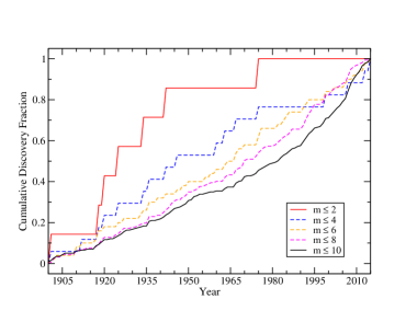
Figure 2.— Cumulative distribution of Galactic novae discovery magnitudes. Despite the expected increase in the discovery rate for fainter novae in recent years, note the striking drop in the discovery of bright novae since $\sim$1950.

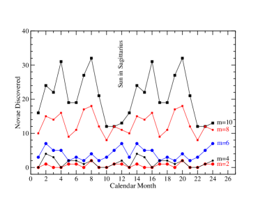
Figure 3.— The number of novae discovered since 1900 plotted as a function of the month of discovery. At the faintest magnitudes a drop in the discovery rate is apparent when the sun is Sagittarius, significantly diminishing the discovery of novae in the direction of the Galactic center.

Surprisingly, novae at the brightest magnitudes appear to be biased toward the northern hemisphere. In Table 2 we show the number of bright novae ($m\leq 5$) discovered north and south of the celestial equator since 1900 as a function of apparent magnitude. At first glance it appears that we may be missing a significant fraction of novae at brighter magnitudes in the southern hemisphere, but the observed sample of novae is small. We can gain some insight into the statistical significance of this apparent asymmetry as follows. For a given magnitude, the probability that $N$ or fewer novae would be discovered in a given hemisphere out of a total of $M$ novae is given by:

$$P_{\leq N,M}=\sum_{N=0}^{N}{M!\over N!(M-N)!}\ 0.5^{M}$$ (1)

Since the excess could have occurred in either hemisphere, we must multiply the probability given in equation (1) by two. For $m=2$ we have $N=2$ and $M=7$, which results in $P_{\leq 2,7}=0.45$. Thus, the fact that only two of the seven novae brighter than $m=2$ have erupted in the southern hemisphere is not particularly surprising. Probabilities for $m=3,4$ and 5 are also given in Table 2. It seems clear that given the small number statistics, we cannot claim any statistically significant bias in bright nova detections to any one hemisphere.

Table 2Equitorial Distribution of Bright Nova Discoveries

$m_{\mathrm{lim}}$	$N_{\mathrm{s}outh}$	$N_{\mathrm{n}orth}$	$N_{\mathrm{t}ot}$	$P$
2	2	5	7	0.45
3	3	8	11	0.23
4	6	11	17	0.33
5	12	21	33	0.16

Table 3Galactic Novae with $m\leq 2$

Name	Date (Y,M,D)	$l$ (∘)	$b$ (∘)	$m_{dis}$	d (kpc)	$E_{B-V}$ (mag)	Ref
V1500 Cyg	1975 8 29	$89.8$	$-0.1$	1.9	$1.5\pm 0.2$	$0.43\pm 0.08$	1,2
CP Pup	1942 11 9	$252.3$	$-0.4$	0.5	$1.5$	$0.25\pm 0.06$	1,2
DQ Her	1934 12 12	$73.2$	$26.4$	1.3	$0.40\pm 0.06$	$0.08$	1,2
RR Pic	1925 5 25	$271.0$	$-25.4$	1.0	0.4	0.02	1,2
V476 Cyg	1920 8 20	$87.4$	$12.4$	2.0	$1.62\pm 0.12$	$0.27\pm 0.12$	1,2
V603 Aql	1918 6 8	$33.2$	$0.8$	$-1.1$	0.33	0.08	1,2
GK Per	1901 2 21	$151.0$	$-10.1$	0.2	$0.46\pm 0.0.03$	0.29	1,2

Nevertheless, evidence for possible incompleteness at bright magnitudes can be appreciated by considering how the rate of discovery of novae reaching apparent magnitude $m$, $N(m)$, has varied over time. Figure 2 shows the cumulative distribution of nova discovery magnitudes during the period between 1900 and 2015. Of the seven novae that reached $m=2$ or brighter, six were discovered in the first half (58 yrs) of this period (see Table 3). Only one nova, Nova Cyg 1975 (V1500 Cyg), which reached $m=1.9$, has been discovered in the second 58 year interval (actually, in the last 73 years!). We can compute the significance of this result by computing the probability that $N$ or fewer novae with $m\leq 2$ would be found within any consecutive 58 year span in the 116 years since 1900. That probability is given by equation (1), where $M-1$ novae must erupt within the same 58 year window. In this case, where $N=1$, we find $P=6\times 0.5^{6}~{}(\rm{one~{}nova})~{}+0.5^{6}~{}(\rm{no~{}novae})=0.11$. Assuming that the true nova rate has been constant over time, a KS test reveals a similar result, namely only a 7% chance that novae with $m\leq 2$ would be distributed as shown in Figure 2. Despite the fact that these probabilities do not rule out 100% completeness for $m\leq 2$ at the $2\sigma$ level, the probabilities are small, and suggest that at least one nova was likely missed in recent years. With only seven of a possible eight $m\leq 2$ novae being detected since 1900, the completeness becomes $\sim 88$%.

Although it appears counterintuitive, Schaefer (2014) points out that incompleteness at brighter magnitudes may be due in part to the evolution of how amateur astronomers survey the sky, which in recent years has turned to the use of telescopes equipped with CCD detectors rather than memorizing the sky and conducting wide-area visual observations. In addition, seasonal effects (i.e., sun in Sagittarius) will also have diminished the observed rate of fainter novae concentrated towards the Galactic center (see Figure 3). As mentioned earlier, after considering a variety of selection effects Schaefer (2014) arrived at a completeness of just 43% for novae brighter than $m=2$. Because only a summary of this work has been published, it is not possible to critically evaluate the assumptions made in arriving at this value. It does, however, seem quite surprising that more than half of the novae reaching second magnitude since 1900 could have been missed. Whether the completeness is close to 90% as estimated above, or whether Schaefer is correct that we have missed more than half of the second magnitude and brighter novae, one thing seems clear, the assumption of 100% completeness for $m\leq 2$ made earlier by Shafter (2002) is likely to be overly optimistic.

In the analysis to follow, we constrain the Galactic nova rate by adopting plausible limits on the completeness of bright novae. Given that it seems difficult to understand how the completeness could be lower than the value determined by Schaefer (2014), we have adopted $c=0.43$ as a lower limit on the completeness of novae with $m\leq 2$. The possibility that all novae with $m\leq 2$ have been detected since 1900 provides a hard upper limit of 100% on the completeness. We argue that the best estimate of the completeness lies between these limits, and follows from two considerations. As described earlier, the sharp drop in the number of $m\leq 2$ novae observed over the past $\sim$60 yr suggests that at least one out of eight bright novae has likely been missed in recent years. If so, a value of $c=0.88$ would seem to offer a reasonable estimate for the completeness of novae with $m\leq 2$. This estimate is supported by considering that even the brightest novae will likely be missed if they erupt within $18^{\circ}$ (1.2 hr) of the sun. Based on this correction alone, the completeness drops to $\sim 90$%. Thus, in computing the models described in the following section, we simply take $c=0.9$ as our best estimate of the completeness for novae with $m\leq 2$. For comparison, we also consider models for $c=0.43$, which we take as a lower limit to the completeness of novae reaching second magnitude or brighter.

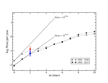
Figure 4.— Cumulative distribution of Novae as a function of peak magnitude. Note the higher average nova rate for novae with $m\mathrel{\hbox{\hbox to0.0pt{\hbox{\lower 4.0pt\hbox{$\sim$}}\hss}\hbox{$<$}}}2$ during the period between $1900-1950$ compared with the period from 1900 to the present. The red square and blue diamond represent the value of log $N(2)$ for the full $1900-2015$ interval corrected for the $c=0.43$ completeness of Schaefer (2014), and for our $c=0.9$ completeness estimate, respectively. The error bars represent the Poisson error for the seven novae discovered with $m\leq 2$. The dashed lines represents the expected increase in the nova rate for an infinite uniform distribution of nova progenitors (log $N\propto 0.6m$), and for an infinite disk distribution (log $N\propto 0.4m$).

3. Model

The annual discovery rate of novae brighter than $m=10$ since 1900 as a function of magnitude is shown in Figure 4. The corrected $m\leq 2$ nova discovery rates for our estimated completeness of $c=0.9$ and the lower completeness advocated by Schaefer (2014) are shown as the blue diamond and the red square, respectively. For comparison, we have also plotted the values of $N(m)$ computed from a sub-sample of novae discovered during the period between 1900 and 1950. We find that the annual discovery rate for novae reaching second magnitude or brighter during this earlier time span is approximately twice that for the full $1900-2015$ period, and is consistent with that expected after applying Schaefer’s incompleteness estimate.

In the analysis to follow, we estimate the Galactic nova rate by extrapolating the local nova rate ($m\leq 2$) to the entire Galaxy based on a model consisting of separate bulge and disk components. The bulge component, $\rho_{b}$, is modeled using a standard de Vaucouleurs (1959) luminosity profile, while The disk nova density, $\rho_{d}$, is assumed to have a double exponential dependence on distance from the Galactic center and on the distance from the Galactic plane.

Table 4Distances of Novae from the Galactic Plane

Nova	$d$ (kpc)	$b$ (∘)	$z$ (kpc)	Ref
CI Aql	5.00	$-0.8$	0.070	1
V356 Aql	1.70	$-4.9$	0.145	1
V528 Aql	2.40	$-5.9$	0.247	1
V603 Aql	0.25	$0.8$	0.003	2
V1229 Aql	1.73	$-5.4$	0.163	1
T Aur	0.96	$-1.7$	0.028	1
IV Cep	2.05	$-1.6$	0.057	1
V394 CrA	10.00	$-7.7$	1.340	1
T CrB	0.90	$48.2$	0.671	1
V476 Cyg	1.62	$12.4$	0.348	1
V1500 Cyg	1.50	$-0.1$	0.003	1
V1974 Cyg	1.77	$-9.6$	0.295	1
V2491 Cyg	13.30	$4.4$	1.020	1
HR Del	0.76	$-14.0$	0.184	1
KT Eri	6.50	$-31.9$	3.435	1
DN Gem	0.45	$14.7$	0.114	1
DQ Her	0.39	$26.4$	0.173	2
V533 Her	0.56	$24.3$	0.230	1
CP Lac	1.00	$-0.8$	0.014	1
DK Lac	3.90	$-5.4$	0.367	1
DI Lac	2.25	$-4.9$	0.192	1
IM Nor	3.40	$3.0$	0.178	1
RS Oph	1.40	$-10.4$	0.253	1
V849 Oph	3.10	$13.5$	0.724	1
V2487 Oph	12.00	$8.0$	1.670	1
GK Per	0.48	$-10.1$	0.084	2
RR Pic	0.52	$-25.4$	0.223	2
CP Pup	1.14	$-0.4$	0.008	2
T Pyx	4.50	$10.2$	0.797	1
U Sco	12.00	$-60.2$	10.413	1
V745 Sco	7.80	$-60.2$	6.769	1
EU Sct	5.10	$-2.8$	0.249	1
FH Ser	0.92	$5.8$	0.093	1
V3890 Sgr	7.00	$-6.4$	0.780	1
LV Vul	0.92	$0.8$	0.013	1
NQ Vul	1.28	$1.3$	0.029	1
CT Ser	1.43	$47.6$	1.056	1
RW UMi	4.90	$33.2$	2.683	1
V3888 Sgr	2.50	$5.4$	0.235	1
PW Vul	1.75	$5.2$	0.159	1
QU Vul	1.76	$-6.0$	0.184	1
V1819 Cyg	7.39	$4.0$	0.515	1
V842 Cen	1.14	$3.6$	0.072	1
QV Vul	2.68	$7.0$	0.327	1
V351 Pup	2.53	$-0.7$	0.031	1
HY Lup	1.80	$9.0$	0.282	1
CP Cru	3.18	$2.2$	0.122	1

Following Bahcall & Soneira (1980) for the Galactic bulge component we have:

$$\rho_{b}(r)=\rho_{b,0}~{}{\mathrm{exp}[-7.669(r/re)^{1/4}]\over(r/r_{e})^{7/8}},$$ (2)

where $r$ is the radial distance from the Galactic center and $r_{e}=2.7$ kpc is the scale parameter for the Galactic bulge. The constant $\rho_{b,0}$ represents the density of bulge novae at the center of the Galaxy.

For the disk component we can write:

$$\rho_{d}(z,x)=\rho_{d,0}~{}exp[-(z/h_{z})-(x-r_{0})/h_{r}],$$ (3)

where $\rho_{d,0}$ is the density of novae at the position of the sun, $z$ is the distance of a nova perpendicular to the Galactic plane, $r_{0}$ is the distance from the Sun to the Galactic center, and $x=[r^{2}-z^{2}]^{1/2}$ is the distance of a nova from the Galactic center in the plane of the Galaxy.

The parameters $h_{r}$ and $h_{z}$ are the scale lengths for the exponential distributions of novae parallel and perpendicular to the Galactic plane, respectively. Bahcall & Soneira (1980) adopted $h_{r}=3.5$ kpc for the radial scale length of the disk and $r_{0}=8$ kpc for the distance from the sun to the Galactic center. More recent studies have suggested a slightly shorter scale length for the disk and a somewhat larger distance to the Galactic center. Here we adopt more recent determinations of $h_{r}=3.0\pm 0.2$ kpc (McMillan, 2011) and $r_{0}=8.33\pm 0.11$ kpc (Chatzopoulos et al., 2015).

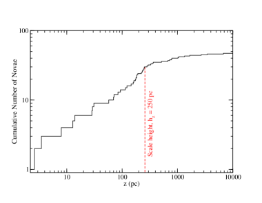
Figure 5.— The $z$ distribution for Galactic novae with known distances. The scale height in the cumulative distribution is given by the value of $z$ corresponding to $N~{}=~{}N_{\mathrm{max}}~{}(1-e^{-1})$. Here we find $z=250$ pc.

Several estimates of the scale height of cataclysmic variables (CVs) perpendicular to the plane of the Galaxy have been made over the years. For example, Patterson (1984) found $z=190$ pc for CVs in general, while Duerbeck (1984) estimated $z=125$ pc for Galactic novae specifically. More recently, Revnivtsev et al. (2008) determined $z=130$ pc for X-ray selected CVs, while Ak et al. (2008) find $z=158\pm 14$ pc for a large sample of Galactic CVs. We have made an independent determination of the scale height for Galactic novae using the distance estimates given in Table 4, which have been taken from Darnley et al. (2012) and Downes & Duerbeck (2000). Figure 5 shows the cumulative distribution of scale heights for the 47 novae in this sample. If we assume novae are distributed as $n(z)=n_{0}~{}\mathrm{exp}(-z/h_{z})$, then for a cumulative distribution where $N(z)=\int_{o}^{z}n(z)dz$, we find that $z=h_{z}$ at $N=N_{\mathrm{max}}(1-e^{-1})$, where $N_{\mathrm{max}}=n_{0}h_{z}$. Taking $N_{\mathrm{max}}=47$, we find $h_{z}\simeq 250$ pc, which is somewhat larger than previous estimates. In the analysis to follow, we will adopt our estimate of $h_{z}=250$ pc. The adopted value of $h_{z}$ sets the local nova rate density, $\rho_{d,0}$, required to normalize the model to $N(2)$. Since the Galactic nova rate is dependent on this normalization, unlike the value of $\rho_{d,0}$, it is not sensitive to the choice of $h_{z}$.

Taken together, $\rho_{b,0}$ and $\rho_{d,0}$ determine the relative contribution of the bulge and disk to the overall Galactic nova rate. At the position of the sun, Bahcall & Soneira (1980) find that the bulge contributes 1/800 of the stellar density. In this case, if we define $\theta(=n_{\mathrm{disk}}/n_{\mathrm{bulge}}$) as the ratio of the specific nova rate of the disk population to that of the bulge population, we find that $\rho_{d,0}/\rho_{b,0}\simeq\theta/79$. Assuming $\theta=1$ and a nova scale height, $h_{z}=250$ pc, this leads to an integrated disk-to-bulge mass ratio of $\sim$15. More recent models for the Galaxy suggest that the bulge component makes up a larger fraction of the Milky Way’s total mass, and that the disk-to-bulge mass ratio, $M_{d}/M_{b}$ is of order 6 (e.g., see McMillan, 2011; Licquia & Newman, 2015). Assuming the relative nova rates follow the integrated bulge and disk masses, a value of $M_{d}/M_{b}=6$ corresponds to a bulge contribution of $\sim$ 1/320 to the total stellar density at the position of the sun. In the calculations to follow we will consider both Bahcall & Soneira (1980) models characterized by $\theta=1.0$ as well as a bulge-enhanced $\theta=0.4$ model. The latter model is equivalent to a $\theta=1.0$ model with a more massive bulge ($M_{d}/M_{b}=6$), where the bulge and disk components produce novae at the same rate per unit mass.

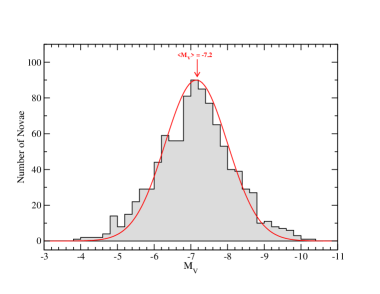
Figure 6.— The absolute magnitude distribution for all known M31 nova candidates through May 2016. The distribution is approximately Gaussian with a mean $<$$M_{V}(\mathrm{M31})$$>$$~{}\simeq-7.2$ and standard deviation of 0.8 magnitudes.

3.1. The Absolute Magnitude Distribution of Novae

Before we can estimate the Galactic nova rate or compute the expected nova rate as function of apparent magnitude, we must specify the absolute magnitude characteristic of Galactic novae. Shafter (2009) has shown that the absolute magnitudes of novae typically range from $M\simeq-5$ to $M\simeq-10$, with the mean peak absolute magnitude for the M31 and the smaller Galaxy samles being given by $<$$M_{V}(\mathrm{M31})$$>$$~{}\simeq-7.2$ and $<$$M_{V}(\mathrm{G})$$>$$~{}\simeq-7.8$, respectively. To bring the M31 sample up to date, we have redetermined absolute magnitude distribution for the full sample of M31 novae through May 2015 given in the online catalog of W. Pietsch using the extinction and color corrections given in Shafter (2009). Figure 6 shows the resulting absolute magnitude distribution. The mean of the distribution remains unchanged with $<$$M_{V}(\mathrm{M31})$$>$$~{}=-7.2$, with a best-fitting Gaussian giving a standard deviation of 0.8 mag.

Selection effects likely bias both the Galactic and M31 nova samples. The Galactic nova sample is affected by extinction, and is almost certainly biased towards more luminous (primarily disk) novae. The M31 Sample is much larger and contains novae from both M31’s bulge and disk components. However, the maximum-light magnitude is based on discovery magnitude rather than confirmed peak magnitude, and thus likely underestimates the absolute magnitude the novae at maximum light. After taking both of these biases into account we adopt $<$$M_{V}$$>$$~{}=-7.5\pm 0.8$ as the best estimate currently available for the average absolute magnitude distribution of Galactic novae at maximum light.

A significant advance in our understanding of extragalactic nova rates came when Kasliwal et al. (2011) discovered a significant population of faint, but fast, novae in M31 that did not appear to follow the canonical maximum-magnitude, rate-of-decline (MMRD) relation for classical novae (e.g., see Downes & Duerbeck, 2000). A typical example of a faint, but fast nova is the recurrent nova M31N 2008-12a mentioned earlier, which only reaches an absolute magnitude $M_{V}~{}\simeq-6$ at maximum light ($m_{V}\simeq 18.5$ at the distance of M31), and fades by two magnitudes from peak in less than two days (Darnley et al., 2015). Such novae have likely been missed in the Galaxy and in previous surveys for novae in M31. As a result of their short recurrence times, such novae could make up a significant fraction of the observed nova rate, and, if properly accounted for could shift the peak absolute magnitude distribution to fainter magnitudes. To explore this possibility, we will also take the M31 absolute magnitude distribution at face value, and consider models where we adopt $<$$M_{V}$$>$$~{}=-7.2\pm 0.8$. Later, we will also consider the possibility that the absolute magnitudes of bulge and disk novae differ.

4. The Galactic Nova Rate

4.1. Direct Extrapolation

Shafter (2002) estimated the global Galactic nova rate by using the Bahcall & Soneira (1980) model to extrapolate the local nova rate (assumed complete for $m\leq 2$) to sufficiently faint magnitudes that the entire galaxy is covered. If we define $R(m)$ as the distance from the sun to a nova of apparent magnitude $m$ we have:

$$R(m)=10^{[1+0.2(m-M_{V}-A_{V}(R))]}$$ (4)

where $M_{V}$ is the absolute visual magnitude at maximum light, and $A_{V}(R)$ is the visual extinction suffered by a nova at distance $R$. The value of $A_{V}$ will be a function of position in the Galaxy, and is approximated here as follows:

$$A_{V}(R)=a_{V}\int_{0}^{R}e^{-z/h_{d}}~{}dR=a_{V}R(h_{d}/z)(1-e^{-z/h_{d}})$$ (5)

where the constant $a_{V}$ represents the extinction in the midplane of the disk, and $h_{d}$ is the scale height of the obscuring dust layer, assumed to drop off exponentially perpendicular to the disk plane. Here, we adopt an average extinction of $a_{V}=1$ mag per kpc in the Galactic midplane, with a scale height perpendicular to the plane, $h_{d}=100$ pc (Spitzer, 1978). Equations (4) and (5) are solved iteratively to determine $R(m)$.

The number of novae per year visible to a given magnitude, $m$, is then given by:

$$N(m)=2\int_{0}^{2\pi}\int_{0}^{\pi/2}\int_{0}^{R(m)}(\rho_{d}+\rho_{b})~{}R^{2}~{}dR~{}\mathrm{cos}~{}b~{}db~{}dl,$$ (6)

where $b$ and $l$ are the Galactic latitude and longitude, respectively, and $\rho_{b}(r)$ and $\rho_{d}(z,x)$ from equations (2) and (3) can be cast in terms of $R$ by noting that

$$r=\big{[}r_{0}^{2}+R^{2}-2Rr_{0}~{}\mathrm{cos}~{}b~{}\mathrm{cos}~{}l\big{]}^{1/2},$$ (7)

$z=R~{}\mathrm{sin}~{}b$, and $x=[r^{2}-z^{2}]^{1/2}$.

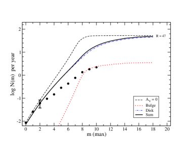
Figure 7.— The cumulative nova rate distribution as a function of peak apparent magnitude is compared with our Galaxy model. The model has been normalized to the observed $N(2)$ assuming 100% completeness. The model predicts a global nova rate of 47 yr^-1. The dotted red line, the dot-dashed blue line, and the solid black line represent the bulge, disk and total rate, respectively. The dashed line represents the extinction-free model with $A_{V}=0$.

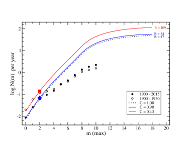
Figure 8.— The same as Figure 7, except that the models have been normalized to the $c=0.9$ and $c=0.43$ completeness-corrected $N(2)$ points shown by the blue diamond and red square, respectively. The dotted line shows the model assuming 100% completeness at $N(2)$ from Fig. 7. Also shown as open circles are the cumulative nova rates based on the period from 1900 to 1950. We note that the $c$=0.43 model matches these data quite well.

Figure 7 shows the expected increase in the observed nova rate as a function of apparent magnitude for the full 1900-2015 sample. The extrapolation is accomplished by integrating equation (4) as a function of apparent magnitude where we assume the average nova has an average absolute magnitude at maximum light of $<$$M_{V}$$>$$~{}=-7.5$. The solid line shows our model for the expected increase in the nova rate with apparent magnitude. As in Shafter (2002), the model has initially been normalized to the observed value of $N(2)$ assuming 100% completeness for $m\leq 2$. The bulge and disk contributions to the overall nova rate are shown as the red dotted and blue dot-dashed curves, respectively. Given that the bulge contributes so little to the nova density at the position of the Sun, these values essentially reflect the nova rate densities of disk novae. The agreement between the observed rates and the model is quite good for novae brighter than $m=2$, with the observed nova rates falling off with increasing apparent magnitude as expected for a disk distribution (log $N\propto 0.4m$). At fainter magnitudes the expected incompleteness in the observed nova rate becomes increasingly apparent. We note that, at magnitudes fainter than $m\simeq 6$, there is a hint that the contribution of bulge novae is beginning to kick in.

Despite the excellent fit of the model to novae with $m\leq 2$, as we have discussed in section 2, the observed nova rates for even these bright novae are likely to be incomplete. Figure 8 shows our model fits to the incompleteness-corrected values of $N(2)$, shown by the blue diamond and the red square for $c=0.9$ and $c=0.43$, respectively. These models assume our best estimate for the mean absolute magnitude of Galactic novae, $<$$M_{V}$$>$$~{}=-7.5$, and produce global Galactic nova rates of $\sim 48$ and $\sim 98$ per year for the $c$=0.9 and $c$=0.43 models, respectively. We note that the rate based on an assumed completeness of 43% for novae brighter than second magnitude is almost exactly what we would expect if we normalized the model to the observed rate during the period between 1900 and 1950, as shown in Figure 4, and assumed 100% completeness during that interval. In both Figures 7 and 8, the overall Galactic nova rates have been approximated as in Shafter (2002) by extrapolating the models to sufficiently faint magnitudes that the entire Galaxy is essentially covered. The slightly higher rates compared with those in Shafter (2002) result from our updated values of $h_{r}$ and $r_{0}$.

Significant limitations of the direct extrapolation approach adopted by Shafter (2002) and reviewed above, are that this method does not provide an uncertainty in the derived nova rates, and that it requires that a specific absolute magnitude for the model novae be specified rather than allowing for a distribution of absolute magnitudes to be considered. A roughly equivalent, but superior approach is to extrapolate the local population of novae to the entire Galaxy using a Monte Carlo simulation.

4.2. Monte Carlo Simulations

In our Monte Carlo simulations, we distribute simulated bulge and disk novae following the scaling laws given in equations (2) and (3) for a range of trial Galactic nova rates, $\nu$. We then record the number of novae brighter than second magnitude, $N_{\nu}(m\leq 2)$, that are produced over the 116 year period covered by the observations. The magnitude of the $i^{th}$ nova is calculated assuming the extinction given by equation (5) over a distance, $R_{i}$, from the sun given by:

$$R_{i}=\big{[}r_{i}^{2}+r_{0}^{2}-2r_{i}r_{0}~{}\mathrm{sin}~{}\theta_{i}~{}\mathrm{cos}~{}\phi_{i}\big{]}^{1/2},$$ (8)

where $\theta$ and $\phi$ are the usual spherical polar coordinates with origin at the center of the Galaxy. For the disk component, $\theta_{i}=\pi/2-\mathrm{tan}^{-1}(z_{i}/x_{i})$, while we assume a uniform distribution in cos $\theta$ for the bulge component. In both cases we assume that the Galaxy is axially symmetric (i.e., a uniform distribution in $\phi$).

We run the simulation $M=10^{5}$ times for each trial nova rate and record the number of times $N_{\nu,i}(m\leq 2)$ from the $i^{th}$ simulation matches the number of novae believed to have reached second magnitude or brighter over the past 116 years. This latter number is simply given by $N_{c}(m\leq 2)=[N_{\mathrm{obs}}/c]$, where $c$ is the assumed observational completeness for $m\leq 2$. To account for variation in the number of $m\leq 2$ novae observed over the past 116 years, our Monte Carlo simulations sample a Poisson distribution (mean of 7) for $N_{\mathrm{obs}}$. Similarly, to account for the uncertainty in $c$, our Monte Carlo simulation samples a distribution, $c_{i}$, which is normally distributed about $c$ with standard deviation $\sigma_{c}$. Figure 9 shows the completeness function and the resulting $N_{c,i}(m\leq 2)$ distribution for our $c=0.9$ models, where we have assumed $\sigma_{c}=0.2$. The most likely estimate of the global nova rate for a given assumed completeness distribution is then given by the value of $\nu$ that produces the largest number of matches between $N_{\nu,i}(m\leq 2)$ and $N_{c,i}(m\leq 2)$. Specifically, the probability of a given nova rate is given by:

$$P(\nu)={\sum_{i=1}^{M}\delta_{N_{\nu,i},N_{c,i}}\over\sum_{\nu=0}^{\infty}\sum_{i=1}^{M}\delta_{N_{\nu,i},N_{c,i}}},$$ (9)

where $\delta$ is the Kronecker delta function.

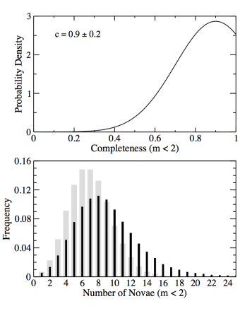
Figure 9.— Top panel: The adopted completeness function for novae with $m\leq 2$ given by $c=0.9\pm 0.2$. Bottom panel: The frequency distribution of $N_{c}(m\leq 2)$ used in the Monte Carlo simulation (black bars), which is based on a Poisson distribution (mean of 7) for $N\mathrm{obs}$ (grey bars) convolved with the completeness function shown in the top panel.

We have run an array of Monte Carlo simulations to explore how the choice of model parameters affect the Galactic nova rate. We initially assumed that the nova rate per unit mass is the same in the disk and bulge (i.e., $\theta=1$), and considered both a disk-to-bulge mass ratio $M_{d}/M_{b}=15$ as found by Bahcall & Soneira (1980) in their pioneering study of the Milky way, and a bulge-enhanced model with $M_{d}/M_{b}=6$. The latter model is equivalent a Bahcall & Soneira (1980) model with a higher specific bulge nova rate given by $\theta=0.4$, which is the value found by Shafter & Irby (2001) based on the spatial distribution of novae in M31. For comparison, we have also computed a pure disk model ($\theta=\infty$) despite the fact that available observations do not support a heavily disk-dominated nova population.

Figure 10 shows a plot of $P(\nu)$ as a function of the trial global nova rate $\nu$ for our most plausible models. Four $c=0.9\pm 0.2$ models are shown representing differences both in the contribution of the Milky Way’s bulge and disk components and in the assumed absolute magnitude distribution of novae. The solid red curve shows the nova rate distribution for a Galactic nova population characterized by $<$$M_{V}$$>$$~{}=-7.5\pm 0.8$ and an assumed disk-to-bulge ratio of 15 ($\theta=1$), while the shaded distribution represents our preferred model with an enhanced bulge component ($\theta=0.4$) that contributes $1/6$ that of the Milky Way’s disk (e.g., see Licquia & Newman, 2015; McMillan, 2011). The peak of this distribution corresponds to a most likely nova rate of $52^{-23}_{+32}$ novae per year, where the uncertainties are 1$\sigma$ errors of an assumed bi-Gaussian distribution (Buys & De Clerk, 1972). Since the local novae ($m\mathrel{\hbox{\hbox to0.0pt{\hbox{\lower 4.0pt\hbox{$\sim$}}\hss}\hbox{$<$}}}2$) are predominately disk novae, an increase in the bulge-to-disk ratio has the effect of shifting the peak of the probability distribution to somewhat higher nova rates.

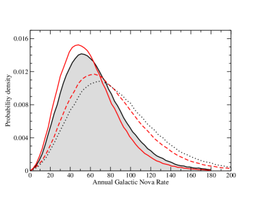
Figure 10.— Galactic nova rate probability density distributions from the Monte Carlo simulations. The shaded region bounded by the black solid line represents our preferred model characterized by $<$$M_{V}$$>$$~{}=-7.5\pm 0.8$ and $\theta=0.4$. The red solid curve shows the distribution for a smaller bulge fraction characterized by $\theta=1.0$. The broken lines represent nova rate probabilities for $<$$M_{V}$$>$$~{}=-7.2\pm 0.8$, with the dashed line for $\theta=1$, and the dotted line for $\theta=0.4$. The peak of a distribution represents the most probable nova rate for a given model.

The broken lines in Figure 10 show nova rate distributions for the two disk-to-bulge ratios assuming the fainter absolute magnitude distribution observed for M31, $<$$M_{V}$$>$$~{}=-7.2\pm 0.8$ (see Fig. 5). These models may be more appropriate for our Galaxy if a significant population of faint and fast novae have escaped detection in previous extragalactic nova surveys (e.g., Kasliwal et al., 2011). If so, $<$$M_{V}$$>$$~{}=-7.5\pm 0.8$ may overestimate the peak luminosity of the Galactic nova distribution. As expected, a lower assumed mean nova luminosity reduces the volume sampled by $m\leq 2$ novae, increases the extrapolation to the entire Galaxy, and results in overall Galactic nova rates as high as $\sim 65$ per year.

In addition to our preferred $c=0.9\pm 0.2$ models, we have also computed model rates based on the low completeness of $c=0.43\pm 0.06$ suggested by Schaefer (2014). As expected, these models result in considerably higher nova rates that reach of order 100 per year in the case of the $<$$M_{V}$$>$$~{}=-7.5\pm 0.8$ models, or even higher if we adopt the lower mean luminosity of $<$$M_{V}$$>$$~{}=-7.2\pm 0.8$. As discussed earlier, we consider it extremely unlikely that the completeness of second magnitude and brighter novae could be below 50%. Thus, the nova rates that result from the $c=0.43\pm 0.06$ models likely represent firm upper limits to the Galactic nova rate.

Table 5Galactic Nova Rate Estimates

				$c=0.9\pm 0.2$				$c=0.43\pm 0.06$
			Bulge	Disk	Total		Bulge	Disk	Total
($\theta$)	($M_{d}/M_{b}$)	($\rho_{d}/\rho_{b})_{\odot}$	Rate (yr-1)	Rate (yr-1)	Rate (yr-1)		Rate (yr-1)	Rate (yr-1)	Rate (yr-1)
$<$$M_{V,\mathrm{disk}}$$>$$~{}=-7.5\pm 0.8,~{}$$<$$M_{V,\mathrm{bulge}}$$>$$~{}=-7.5\pm 0.8$
1.0	15	800	$3.0_{-1.4}^{+1.9}$	$45_{-21}^{+28}$	$48_{-22}^{+30}$		$5.7_{-1.9}^{+2.5}$	$84_{-28}^{+37}$	$90_{-30}^{+40}$
0.4 (1.0)	15 (6)	320	$7.4_{-3.4}^{+4.6}$	$45_{-21}^{+27}$	$52_{-24}^{+32}$		$14_{-4.6}^{+6.3}$	$84_{-27}^{+38}$	$98_{-32}^{+44}$
$\infty$	$\infty$	$\infty$	…	$45_{-19}^{+27}$	$45_{-19}^{+27}$		…	$86_{-30}^{+37}$	$86_{-30}^{+37}$
$<$$M_{V,\mathrm{disk}}$$>$$~{}=-7.2\pm 0.8,~{}$$<$$M_{V,\mathrm{bulge}}$$>$$~{}=-7.2\pm 0.8$
1.0	15	800	$4.0_{-1.8}^{+2.3}$	$60_{-27}^{+35}$	$64_{-29}^{+37}$		$7.6_{-2.5}^{+3.2}$	$112_{-37}^{+48}$	$120_{-40}^{+51}$
0.4 (1.0)	15 (6)	320	$9.7_{-4.3}^{+6.0}$	$58_{-26}^{+36}$	$68_{-30}^{+42}$		$19_{-6.3}^{+8.0}$	$111_{-38}^{+48}$	$130_{-44}^{+56}$
$\infty$	$\infty$	$\infty$	…	$60_{-27}^{+37}$	$60_{-27}^{+37}$		…	$112_{-37}^{+49}$	$112_{-37}^{+49}$
$<$$M_{V,\mathrm{disk}}$$>$$~{}=-7.8\pm 0.8,~{}$$<$$M_{V,\mathrm{bulge}}$$>$$~{}=-7.2\pm 0.8$
1.0	15	800	$2.3_{-1.2}^{+1.8}$	$34_{-18}^{+26}$	$36_{-19}^{+28}$		$4.3_{-1.4}^{+1.9}$	$65_{-21}^{+29}$	$69_{-23}^{+31}$
0.4 (1.0)	15 (6)	320	$5.7_{-2.6}^{+3.6}$	$34_{-15}^{+21}$	$40_{-18}^{+25}$		$11_{-3.6}^{+4.7}$	$64_{-21}^{+28}$	$75_{-25}^{+33}$
$\infty$	$\infty$	$\infty$	…	$35_{-16}^{+21}$	$35_{-16}^{+21}$		…	$65_{-23}^{+30}$	$65_{-23}^{+30}$

A summary of our full array of models is given in Table 5. Each model is described in columns $1-3$, which give the ratio of the specific disk-to-bulge nova rates, $\theta$, the disk-to-bulge mass ratio, $M_{d}/M_{b}$, and the corresponding disk-to-bulge nova density ratio at the position of the sun, ($\rho_{d}/\rho_{b})_{\odot}$. The derived nova rates are not sensitive to the adopted model parameters such as the bulge scale parameter, $r_{e}$, or the disk scale length, $h_{r}$, and height, $h_{z}$. The local nova rate density $\rho_{d,0}$, however, does depend on the assumed scale height of novae in the disk. Values of $\rho_{d,0}$ for three representative values of $h_{z}$ are given in Table 6.

Table 6Local Nova Rate Density Estimates

	$c=1.0$	$c=0.9\pm 0.2$	$c=0.43\pm 0.06$
$h_{z}$	$\rho_{d,0}$	$\rho_{d,0}$	$\rho_{d,0}$
(pc)	(kpc-3 yr-1)	(kpc-3 yr-1)	(kpc-3 yr-1)
$<$$M_{V,\mathrm{disk}}$$>$$~{}=-7.5,~{}$$<$$M_{V,\mathrm{bulge}}$$>$$~{}=-7.5$
125	0.18	0.21	0.39
150	0.16	0.19	0.34
250	0.11	0.13	0.24
$<$$M_{V,\mathrm{disk}}$$>$$~{}=-7.2,~{}$$<$$M_{V,\mathrm{bulge}}$$>$$~{}=-7.2$
125	0.23	0.26	0.50
150	0.21	0.25	0.49
250	0.15	0.17	0.32
$<$$M_{V,\mathrm{disk}}$$>$$~{}=-7.8,~{}$$<$$M_{V,\mathrm{bulge}}$$>$$~{}=-7.2$
125	0.12	0.13	0.28
150	0.11	0.12	0.25
250	0.074	0.082	0.18

We note that Galactic nova rates determined in our Monte Carlo simulations are slightly lower than those found in the direct extrapolation described in the previous section. This difference is the result of the fact that for a given apparent magnitude, the volume, $V(M_{V})$, sampled is not directly proportional to $M_{V}$, but rather $V(M_{V})~{}\propto 10^{-0.6M_{V}}$. Thus, the average volume sampled for a Gaussian distribution of absolute magnitudes is larger than the volume sampled assuming a single average absolute magnitude alone. In other words, $<$$V(M_{V})$$>$ $>$ $V($$<$$M_{V}$$>$). The larger volume sampled for novae with $m\leq 2$ results in a smaller extrapolation, and therefore a lower overall nova rate.

4.2.1 The Effect of Differing Nova Populations

For some time there has been speculation that that there may be two distinct populations of novae: a bulge population characterized by relatively slow and dim novae, and a disk population characterized by somewhat brighter novae that lie closer to the Galactic plane and generally evolve more quickly (della Valle et al., 1992). The evidence for two populations finds some support from observations showing that novae can be divided into two classes based upon the character of their spectra shortly after eruption. Although all novae display prominent Balmer emission shortly after eruption, the so-called “Fe II novae”, are characterized by relatively narrow ($\sim$1000 km s^-1 FWHM) Fe II emission features that exhibit P-Cyg profiles near maximum light, while the “He/N novae” show prominent and broad ($\mathrel{\hbox{\hbox to0.0pt{\hbox{\lower 4.0pt\hbox{$\sim$}}\hss}\hbox{$>$}}}$2500 km s^-1 FWHM) He I and N emission features, but without the Fe II emission Williams (1992). The work of della Valle & Livio (1998) showed that the He/N novae cluster close to the Galactic plane and tend to be fast and bright relative to the Fe II class.

Given the possible existence of two classes of novae, we have also computed nova rate models that are characterized by different average peak luminosities and specific nova rates in the Galactic bulge and disk. Specifically, we have considered a two-component Galaxy model where disk novae are characterized by $<$$M_{V}$$>$$~{}=-7.8$ and bulge novae by $<$$M_{V}$$>$$~{}=-7.2$. Since the $m\leq 2$ disk novae used in the normalization are more luminous, they extend to a larger volume of the Galaxy. Thus, both the density of novae in the vicinity of the sun ($\rho_{d,0}$) and the extrapolated global Galactic nova rate are significantly reduced. Bulge-dominated ($\theta=0.4$) models produce generally higher rates because the normalization is set by nearby novae that belong overwhelmingly to the disk, whereas disk dominated models ($\theta=\infty$) produce lower rates because there is no contribution from the bulge.

Table 7Predicted Visibility of Galactic Novae

	$c=0.9\pm 0.2$			$c=0.43\pm 0.06$
	$\theta=1.0$	$\theta=0.4$		$\theta=1.0$	$\theta=0.4$
$m_{\mathrm{l}im}$	$N$ (yr${}^{-1})$	$N$ (yr${}^{-1})$		$N$ (yr${}^{-1})$	$N$ (yr${}^{-1})$
$<$$M_{V,\mathrm{disk}}$$>$$~{}=-7.5,~{}$$<$$M_{V,\mathrm{bulge}}$$>$$~{}=-7.5$
2.0	0.1	0.1		0.1	0.1
4.0	0.4	0.4		0.7	0.7
6.0	1.5	1.5		2.8	2.8
8.0	5.2	5.4		9.7	10
10.0	14	14		25	27
12.0	23	25		44	48
14.0	32	35		60	66
16.0	38	42		72	79
18.0	42	46		80	87
20.0	45	49		84	92
$<$$M_{V,\mathrm{disk}}$$>$$~{}=-7.2,~{}$$<$$M_{V,\mathrm{bulge}}$$>$$~{}=-7.2$
2.0	0.1	0.1		0.1	0.1
4.0	0.4	0.4		0.7	0.7
6.0	1.6	1.6		3.0	3.0
8.0	5.8	5.8		11	11
10.0	16	17		30	32
12.0	29	31		55	59
14.0	41	44		77	84
16.0	50	54		94	102
18.0	56	60		105	114
20.0	59	63		111	121
$<$$M_{V,\mathrm{disk}}$$>$$~{}=-7.8,~{}$$<$$M_{V,\mathrm{bulge}}$$>$$~{}=-7.2$
2.0	0.1	0.1		0.1	0.1
4.0	0.3	0.3		0.7	0.7
6.0	1.3	1.4		2.6	2.6
8.0	4.5	4.7		8.7	8.9
10.0	11	12		21	22
12.0	19	20		35	38
14.0	25	27		47	51
16.0	29	33		56	61
18.0	32	36		62	67
20.0	34	38		65	70

4.2.2 Bulge Rates

In addition to summarizing Galactic nova rates produced by the various models, Table 5 also breaks down the corresponding bulge (and disk) contributions to the overall rate. As with the overall rates, the bulge nova rates also depend on the adopted Galaxy model, absolute magnitude distribution, and completeness at bright magnitudes, $c$. Our $c=0.9\pm 0.2$ models predict Galactic bulge rates ranging between $\sim 3$ yr^-1 and $\sim 10$ yr^-1 depending on assumed parameters. The lowest bulge rates result from our $\theta=1$, $<$$M_{V}$$>$$~{}=-7.5$ models, with the $\theta=0.4$, $<$$M_{V}$$>$$~{}=-7.2$ variations producing significantly higher rates. As expected, the $c=0.43\pm 0.06$ models produce bulge rates that are approximately a factor of two higher. The bulge rate of $13.8\pm 2.6$ found by Mróz et al. (2015), would appear most consistent with either the bulge-enhanced ($\theta=0.4$), $c=0.9\pm 0.2$ models or the $\theta=1$, $c=0.43\pm 0.06$ models, which produce bulge nova rates of $\sim 7-10$ yr^-1 and $15-20$ yr^-1, respectively.

4.2.3 The Predicted Nova Rate as a Function of Apparent Magnitude

In addition to estimating the overall Galactic nova rate, our Monte Carlo simulations have been used to predict how the number of Galactic novae should increase with apparent magnitude. Assuming the most probable overall nova rates from Table 5, we show in Table 7 the predicted increase in the number of novae visible as a function of apparent magnitude for our $\theta=1.0$ and $\theta=0.4$ models with and assumed completenesses of $c=0.9\pm 0.2$ and $c=0.43\pm 0.06$. These predictions can be compared with the results from several ongoing and planned all-sky surveys such as ASAS-SN and ZTF once they are available, and used to differentiate between the various Galactic nova rate models presented here.

5. Comparison with Extragalactic Nova Rates

In recent years evidence has been building that extragalactic nova rates, which have been determined primarily through synoptic surveys often with sparse temporal sampling, may have been systematically underestimated. In particular, Curtin et al. (2015) and Shara et al. (2016) have recently argued that the nova rate in the giant Virgo elliptical galaxy M87 is likely $2-3$ times larger than previously thought, with the latter authors suggesting that the $K$-band luminosity-specific nova rates (LSNRs) of all galaxies may be $\sim 3-4$ times higher than the previous average of $\sim$2 novae per year per $10^{10}$ solar luminosities in $K$ (Shafter et al., 2014).

As mentioned earlier, the work of Kasliwal et al. (2011) has shown that a population of faint and fast novae, which deviate from the canonical MMRD relation may exist. Owing to their intrinsically low peak luminosities and their rapid declines, such novae have almost certainly been missed in previous magnitude-limited and low cadence synoptic surveys for novae in M31. Because these novae deviate so strongly from the assumed MMRD, they have not been properly accounted for when the surveys were corrected for completeness. In most surveys, the incompleteness, and thus the final nova rates, have likely been underestimated.

The generally accepted nova rate for M31 is $65^{+16}_{-15}$ (Darnley et al., 2006). This value has been called into question recently by Chen et al. (2016) who have computed population synthesis models to estimate nova rates in galaxies with differing star formation histories and morphological types. They estimate a global nova rate for M31 of 97 yr^-1. In another study, Soraisam et al. (2016) corrected the nova samples of Arp (1956) and Darnley et al. (2006) for bias against the discovery of fast novae in these synoptic surveys. Based on these corrections, they estimate a global nova rate for M31 of order 106 yr^-1. Thus, the most recent estimates suggest the nova rate in M31 could be as high as $\sim 100$ yr^-1. The stellar mass of M31 relative to the Galaxy is not precisely known, but we can compare estimates for the integrated $K$-band luminosity, which should reflect the mass difference. For the Galaxy, we adopt $M_{V}=-20.6$ (Bahcall & Soneira, 1980), while for M31 we have $m_{V}=3.44$ (de Vaucouleurs et al., 1991) and $(m-M)_{0}=24.38$ (Freedman et al., 2001), yielding $M_{V}(\mathrm{M31})=-20.94$. Since both galaxies have similar morphological types (Sbc), their integrated $V-K$ colors should be similar, and in both cases we adopt $<$$V-K$$>~{}\simeq 3.25$ (Aaronson, 1978). Thus, we estimate $M_{K}(\mathrm{M31})=-24.19$ and $M_{K}(\mathrm{MW})=-23.85$, which corresponds to a luminosity ratio, $L_{K,\mathrm{MW}}/L_{K,\mathrm{M31}}\simeq 0.73$. Assuming the relative nova rates follow the relative luminosities, based on a comparison with M31, we expect a nova rate in the Galaxy of between $\sim$50 yr^-1 and $\sim 70$ yr^-1, depending on whether we adopt the Darnley et al. (2006) or the recent estimates. Generally speaking, these estimates are in good agreement with an average of the rates given in Table 5. The corresponding LSNRs for both M31 and the Galaxy are $\sim 8.5\pm 1.5$ novae per year per $10^{10}$ $L_{\odot,K}$. This value is in excellent agreement with LSNRs of $9.2^{+2.7}_{-3.0}$ and $8.6\pm 2.7$ novae per year per $10^{10}$ $L_{\odot,K}$ recently found by Shara et al. (2016) and Mróz (2016) for M87 and the Galactic bulge, respectively.

6. Conclusions

By considering how the observed nova rate in the Galaxy varies with apparent magnitude, Shafter (2002) estimated the overall Galactic nova rate by extrapolating the observed rate in the vicinity of the sun ($m\mathrel{\hbox{\hbox to0.0pt{\hbox{\lower 4.0pt\hbox{$\sim$}}\hss}\hbox{$<$}}}2$), which was assumed to be complete, to the entire Galaxy using a two-component disk-plus-bulge model similar to that employed by Bahcall & Soneira (1980) to model the stellar density in the Milky Way. In this paper, we have reconsidered and improved the Shafter (2002) analysis in two important respects. First, we have considered important corrections for the incompleteness in the observed sample of nearby novae with $m\leq 2$, and secondly, we have employed a Monte Carlo analysis to extrapolate the local nova rate to the entire galaxy. The Monte Carlo analysis has the advantage of allowing us to consider a distribution of nova absolute magnitudes rather than a single mean value as in Shafter (2002) and to better assess the uncertainties in our derived Galactic nova rate estimates. In addition to these two principal improvements, we have also updated the sample of novae that have become available over the past 15 years (albeit with no new novae discovered with $m\leq 2$), and updated the values for several Galaxy model parameters.

Galactic nova rate estimates based upon our array of models have been summarized in Table 5. We have considered disk to bulge mass ratios, $M_{d}/M_{b}=15$, as found by Bahcall & Soneira (1980), as well as a more massive bulge model characterized by $M_{d}/M_{b}=6$. The latter model is equivalent to a Bahcall & Soneira (1980) model where the specific nova rate in the disk is just 0.4 times that of the bulge ($\theta=1.0$ vs $\theta=0.4$). Our models have been normalized assuming correction factors of $c=0.9\pm 0.2$ and $c=0.43\pm 0.06$ for the observed fraction of novae that reached second magnitude or brighter since 1900. The $c=0.9\pm 0.2$ models represent our best estimate of the actual completeness of novae with $m\leq 2$ observed since 1900, with the $c=0.43\pm 0.06$ models representing a likely lower limit to the completeness, and thus an upper limit to the nova rate. We have also considered models assuming two different nova absolute magnitude distributions. Based on both Galactic and M31 nova samples, we consider $<$$M_{V}$$>$$~{}=-7.5\pm 0.8$ to represent the best estimate available for the absolute magnitude distribution of Galactic novae. For comparison, we also considered a somewhat fainter absolute magnitude distribution given by $<$$M_{V}$$>$$~{}=-7.2\pm 0.8$, which is characteristic of the observed distribution in M31. The latter absolute magnitude distribution may be more appropriate if there is a significant population of faint and “fast” novae that have hitherto largely escaped detection in existing surveys. Our models produce Galactic nova rates that typically range from $\sim$50 per year to in excess of 100 per year in the case where we are observing only 43% of the novae reaching $m=2$ or brighter. We have also considered models where the absolute magnitudes of the disk and bulge nova rates differ. If disk novae are significantly more luminous than bulge novae (e.g., $<$$M_{V,\mathrm{disk}}$$>$$=-7.8\pm 0.8$ and $<$$M_{V,\mathrm{bulge}}$$>$$=-7.2\pm 0.8$), then somewhat lower nova rates result, falling in the range of $\sim 35$ to $\sim$75 per year.

Since we currently know little about how nova properties may vary with population, and the completeness estimates are similarly uncertain, arriving at a definitive estimate for the Galactic nova rate based on existing data is not possible. Taking an average of the most plausible $c=0.9\pm 0.2$ rates from Table 5 (the $\theta=1$ and $\theta=0.4$ models), yields a value of $50_{-23}^{+31}$ yr^-1, which we adopt as the best estimate currently available for the nova rate in the Galaxy. Rates on the order of 100 per year are possible in the event that we have missed roughly half of the novae that have reached second magnitude or brighter over the last century. Despite the large uncertainties, the rates derived in the present study point towards significant increases over recent estimates, and bring the Galactic nova rate into better agreement with that expected based on comparison with the latest results from extragalactic surveys.

References

- Aaronson (1978) Aaronson, M. 1978, ApJ, 221, 103
- Ak et al. (2008) Ak, T., Bilir, S., Ak, S., Eker, Z. 2008, NewA, 13, 133
- Arp (1956) Arp, J. C. 1956, AJ, 61, 15
- Bahcall & Soneira (1980) Bahcall, J. N., Soneira, R. M. 1980, ApJS, 44, 73
- Buys & De Clerk (1972) Buys, T. S., & De Clerk, K. 1972, AnaCh, 44, 1273
- Chatzopoulos et al. (2015) Chatzopoulos, S., Fritz, T. K., Gerhard, O., Gillessen, S., Wegg, C., et al. 2015, MNRAS, 447, 948
- Chen et al. (2016) Chen, H.-L., Woods, T. E., Yungelson, L. R., Gilfanov, M., Han, Z. 2016, MNRAS, 458, 2916
- Curtin et al. (2015) Curtin, C., Shafter, A. W., Pritchet, C. J., Neill, J. D., Kundu, A., Maccarone, T. J. 2015, ApJ, 811, 34
- Darnley et al. (2006) Darnley, M. J., Bode, M. F., Kerins, E., Newsam, A. M., An, J., et al. 2006, MNRAS, 369, 257
- Darnley et al. (2012) Darnley, M. J., Ribeiro, V. A. R. M., Bode, M. F., Hounsell, R. A., Williams, R. P. 2012, ApJ, 746, 61
- Darnley et al. (2015) Darnley, M. J., Henze, M., Steele, I. A., Bode, M. F., Ribeiro, V. A. R. M., et al. 2015, A&A, 580, 45
- della Valle et al. (1992) della Valle, M., Bianchini, A., Livio, M., Orio, M. 1992, A&A, 266, 232
- della Valle & Livio (1994) della Valle, M., Livio, M. 1994, A&A, 286, 786
- della Valle & Livio (1998) della Valle, M., Livio, M. 1998, ApJ, 506, 818
- de Vaucouleurs (1959) de Vaucouleurs, G. 1959, Handbuch der Physik, 53, 311
- de Vaucouleurs et al. (1991) de Vaucouleurs, G., de Vaucouleurs, A., Corwin, Jr., H. G., et al. 1991, Third Reference Catalogue of Bright Galaxies. Volume I: Explanations and references. Volume II: Data for galaxies between 0h and 12h. Volume III: Data for galaxies between 12h and 24h
- Downes & Duerbeck (2000) Downes, R. A. & Duerbeck, H. W. 2000, AJ, 120, 2007
- Duerbeck (1984) Duerbeck, H. W. 1984, Ap&SS, 99, 363
- Duerbeck (1987) Duerbeck, H. W. 1987, SSRv, 45, 1
- Freedman et al. (2001) Freedman, W. L., Madore, B. F., Gibson, B. K., Ferrarese, L., Kelson, D. D. et al. 2001, ApJ, 553, 47
- Henze et al. (2015a) Henze, M., Ness, J.-U., Darnley, M. J., Bode, M. F., Williams, S. C., et al. 2015a, A&A, 580, 45
- Henze et al. (2015b) Henze, M., Darnley, M. J., Kabashima, F., Nishiyama, K., Itagaki, K., Gao, X. 2015b, A&A, 582, 8
- José et al. (2006) José, J., Hernanz, M., Iliadis, C. 2006, NuPhA, 777, 550
- Kasliwal et al. (2011) Kasliwal, M. M., Cenko, SB, Kulkarni, S. R., Ofek, E. O., Quimby, R. M., & Rau, A. 2011, ApJ, 735, 94
- Kato et al. (2014) Kato, M., Saio, H., Hachisu, I., Nomoto, K. 2014, ApJ, 793, 136
- Licquia & Newman (2015) Licquia, T. C. & Newman, J. A. 2015, ApJ, 806, 96
- McMillan (2011) McMillan, P. J. 2011, MNRAS, 414, 2446
- Miyaji et al. (1980) Miyaji, S., Nomoto, K., Yokoi, K., Sugimoto, D. 1980, PASJ, 32, 303
- Mróz et al. (2015) Mróz, P., Udalski, A., Poleski, R., Soszyński, I., Szymański, M. K., et al. 2015, ApJS, 219, 26
- Mróz (2016) Mróz, P. 2016, to be published in The Golden Age of Cataclysmic Variables and Related Objects - III, 7–12 September 2015, Palermo, Italy
- Patterson (1984) Patterson, J. 1984, ApJS, 54, 443
- Revnivtsev et al. (2008) Revnivtsev, M., Sazonov, S., Krivonos, R., Ritter, H., Sunyaev, R. 2008, A&A, 489, 1121
- Schaefer (2014) Schaefer, B. E. 2014, AAS #224, 306.04
- Shafter (2009) Shafter, A. W., Rau, A., Quimby, R. M., Kasliwal, M. M., Bode, M. F. 2009, ApJ, 690, 1148
- Shafter (1997) Shafter, A. W. 1997, ApJ, 487, 226
- Shafter et. al. (2000) Shafter, A. W. Ciardullo, R. & Pritchet, C. J. 2000, ApJ, 530, 193
- Shafter & Irby (2001) Shafter, A. W. & Irby, B. K. 2001, ApJ, 562, 749
- Shafter (2002) Shafter, A. W. 2002, in Classical Nova Explosions: International Conference on Classical Nova Explosions. AIP Conference Proceedings, Volume 637, pp. 462
- Shafter et al. (2014) Shafter, A. W., Curtin, C., Pritchet, C. J., Bode, M. F., Darnley, M. J. 2014, ASPC, 490, 77.
- Shafter et al. (2015) Shafter, A. W., Henze, M., Rector, T. A., Schweizer, F., Hornoch, K., et al. 2015, ApJS, 216, 34
- Shara et al. (2016) Shara, M. M., Doyle, T., Lauer, T. R., Zurek, D., Neill, J. D. 2016, arXiv160200758S
- Sharov (1972) Sharov, A. S. 1972, SvA, 16, 41
- Soraisam & Gilfanov (2015) Soraisam, M. D., Gilfanov, M. 2015, A&A, 583, 140
- Soraisam et al. (2016) Soraisam, M. D., Gilfanov, M., Wolf, W. M., Bildsten, L. 2016, MNRAS, 455, 668
- Spitzer (1978) Spitzer, L. 1978, Physical processes in the interstellar medium. New York Wiley-Interscience
- Starrfield et al. (2016) Starrfield, S., Iliadis, C., Hix, W. R. 2016, PASP, 128, 1001
- Tang et al. (2014) Tang, S., Bildsten, L., Wolf, W. M., Li, K. L., Kong, A. K. H., et al. 2014, ApJ, 786, 61
- van den Bergh & Younger (1987) van den Bergh, S. & Younger, P. F. 1987, A&AS, 70, 125
- Williams (1992) Williams, R. E. 1992, AJ, 104, 725
- Wolf et al. (2013) Wolf, W. M., Bildsten, L., Brooks, J., Paxton, B. 2013, ApJ, 777, 136