A moving mesh unstaggered constrained transport scheme for magnetohydrodynamics

Abstract

We present a constrained transport (CT) algorithm for solving the 3D ideal magnetohydrodynamic (MHD) equations on a moving mesh, which maintains the divergence-free condition on the magnetic field to machine-precision. Our CT scheme uses an unstructured representation of the magnetic vector potential, making the numerical method simple and computationally efficient. The scheme is implemented in the moving mesh code Arepo. We demonstrate the performance of the approach with simulations of driven MHD turbulence, a magnetized disc galaxy, and a cosmological volume with primordial magnetic field. We compare the outcomes of these experiments to those obtained with a previously implemented Powell divergence-cleaning scheme. While CT and the Powell technique yield similar results in idealized test problems, some differences are seen in situations more representative of astrophysical flows. In the turbulence simulations, the Powell cleaning scheme artificially grows the mean magnetic field, while CT maintains this conserved quantity of ideal MHD. In the disc simulation, CT gives slower magnetic field growth rate and saturates to equipartition between the turbulent kinetic energy and magnetic energy, whereas Powell cleaning produces a dynamically dominant magnetic field. Such difference has been observed in adaptive-mesh refinement codes with CT and smoothed-particle hydrodynamics codes with divergence-cleaning. In the cosmological simulation, both approaches give similar magnetic amplification, but Powell exhibits more cell-level noise. CT methods in general are more accurate than divergence-cleaning techniques, and, when coupled to a moving mesh can exploit the advantages of automatic spatial/temporal adaptivity and reduced advection errors, allowing for improved astrophysical MHD simulations.

1 Introduction

The need for performing accurate, spatially- and temporally-adaptive magnetohydrodynamic (MHD) simulations in astrophysics is evident. Magnetic fields are prevalent in a range of astrophysical systems from cosmological (Marinacci et al., 2015), cluster (McCourt et al., 2012), and galaxy (Wang & Abel, 2009; Dubois & Teyssier, 2010; Beck et al., 2012; Pakmor, Marinacci & Springel, 2014; Rieder & Teyssier, 2016) scales, to the turbulent interstellar medium (Collins et al., 2012; Federrath & Klessen, 2012; Myers et al., 2013; Federrath, 2015), accretion around black holes (McKinney et al., 2014; Sa̧dowski et al., 2014), mergers of compact objects (Zhu et al., 2015), tidal disruption events (Kelley, Tchekhovskoy & Narayan, 2014), and others. Often, these systems exhibit a large dynamic range in physical and temporal scales. For example, a simulation box may contain significant regions of low density gas combined with concentrated volumes where most of the material is present and dynamical time-scales are the shortest. Adaptive, minimally-diffusive schemes are necessary for simulating such configurations precisely, given the limitations in memory and computation speed of modern supercomputing technology.

Solving the ideal MHD equations is more challenging numerically than evolving the inviscid, magnetic-free Euler equations, due to the divergence free nature of the magnetic field ($\nabla\cdot\mathbf{B}=0$) from Maxwell’s equations. This condition needs to be maintained in the discrete representation of the fluid in order for a numerical solver to be both stable and accurate. The finite-volume method is a standard approach for solving the Euler equations on a mesh. However, this technique fails for the MHD equations because divergence errors can cause the magnetic fields to blow up. On static, regular, Cartesian meshes, the state-of-the art solution to this problem is to use the constrained transport (CT) scheme (Evans & Hawley, 1988), which maintains the discretized divergence of $\mathbf{B}$ to zero exactly at machine precision. This method originally comes from the staggered-mesh method of Yee (1966) for electromagnetism in a vacuum. Conceptually, the $\nabla\cdot\mathbf{B}=0$ constraint is exactly maintained with CT by representing the magnetic field as cell face-averaged quantities (as opposed to the usual choice of volume-averages), and making use of Stokes’ Theorem.

The CT method does not generalize easily, however, to moving meshes (e.g. Springel 2010, Duffell & MacFadyen 2011, Gaburov, Johansen & Levin 2012), and may not be at all applicable to meshless Lagrangian approaches (e.g. smoothed particle hydrodynamics (SPH) Tricco 2015, or the volume ‘overlap’ method of Hopkins 2015; Hopkins & Raives 2016). Consequently, numerical solvers in a Lagrangian setting have resorted to magnetic field cleaning schemes, such of those of Dedner et al. (2002) and Powell et al. (1999), which, while stable, may have unwanted numerical side-effects. This has been an unfortunate situation for these Lagrangian approaches, because otherwise they offer many advantages over static mesh codes, including automatic spatial adaptability, significantly larger CFL-limited timesteps for high Mach number flows, and reduced advection errors.

In this paper, we overcome this limitation by developing and presenting an unstaggered CT method for solving the 3D ideal MHD equations on moving meshes. Seminal ideas for our new technique come from our recent paper Mocz, Vogelsberger & Hernquist (2014), where we generalized the staggered CT approach to a 2D moving mesh. However, we have now modified and refined the ideas further to improve the efficiency and simplicity of the algorithm. The new scheme employs an unstructured (cell-centred) formulation, using the magnetic vector potential, which makes it straightforward to adapt to moving mesh codes. We have implemented this new unstaggered CT method into Arepo (Springel, 2010), which is a state-of-the-art moving mesh code for astrophysical flows.

We provide a brief history of the development of moving mesh MHD solvers for astrophysics, to place our work in context. The finite-volume moving mesh formulation for the Euler equations was developed for astrophysical simulations by Springel (2010). The MHD equations were first solved on a moving mesh with some success in Duffell & MacFadyen (2011); Pakmor, Bauer & Springel (2011); Gaburov, Johansen & Levin (2012), using the Dedner hyperbolic divergence-cleaning scheme. However, numerical limitations of these approaches have been reported. Pakmor & Springel (2013) implemented a Powell cleaning technique for a moving mesh, which showed improved stability (even in very dynamic environments) but larger divergence errors (but still small enough in many cases to not affect dynamics). The Powell scheme has been used for science applications, including the study of magnetic fields in disc galaxies (Pakmor, Marinacci & Springel, 2014), Carbon-Oxygen white dwarf mergers (Zhu et al., 2015), and the large-scale properties of simulated cosmic magnetic fields and effects on the galaxy population (Marinacci et al., 2015; Marinacci & Vogelsberger, 2016). Mocz, Vogelsberger & Hernquist (2014) extended the standard CT algorithm to a 2D moving Voronoi mesh, keeping track of face-averaged magnetic fields and remapping onto new faces that appear as the mesh changes connectivity. We have simplified this idea in the present paper to easily and efficiently extend it to a 3D moving mesh code.

The paper is organized as follows. We present the unstaggered moving mesh CT scheme in Section 2. In Section 3 we show the results of test problems (Orszag-Tang, circularly polarized Alfvén wave, turbulent box, magnetic disc, cosmological volume) and compare with Powell cleaning. We discuss the advantages of the new algorithm and offer concluding remarks in Section 4.

2 Numerical Method

In this section we describe our numerical method for an unstructured CT solver on a moving Voronoi mesh. The ideal MHD equation and some notation are presented in Section 2.1. The CT algorithm is detailed in Section 2.2. A procedure for implementing the approach in a periodic domain are discussed in Section 2.3.

2.1 The magnetohydrodynamic equations

The ideal MHD equations are represented in conservation law form by:

$$\frac{\partial\mathbf{U}}{\partial t}+\nabla\cdot\mathbf{F}=0$$ (1)

where $\mathbf{U}$ is the vector of the conserved variables and $\mathbf{F}(\mathbf{U})$ is the flux:

$$\mathbf{U}=\begin{pmatrix}\rho\\ \rho\mathbf{v}\\ \rho e\\ \mathbf{B}\end{pmatrix},\,\,\,\,\,\,\mathbf{F}(\mathbf{U})=\begin{pmatrix}\rho\mathbf{v}\\ \rho\mathbf{v}\mathbf{v}^{T}+p-\mathbf{B}\mathbf{B}^{T}\\ \rho e\mathbf{v}+p\mathbf{v}-\mathbf{B}(\mathbf{v}\cdot\mathbf{B})\\ \mathbf{B}\mathbf{v}^{T}-\mathbf{v}\mathbf{B}^{T}\end{pmatrix}$$ (2)

and $p=p_{\rm gas}+\frac{1}{2}\mathbf{B}^{2}$ is the total gas pressure, $e=u+\frac{1}{2}\mathbf{v}^{2}+\frac{1}{2\rho}\mathbf{B}^{2}$ is the total energy per unit mass, and $u$ is the thermal energy per unit mass. The equation of state for the fluid is given by the ideal gas law $p=(\gamma-1)\rho u$.

The mass density ($\rho$), momentum density ($\rho\mathbf{v}$), and energy density ($\rho e$) are evolved according to the second-order, Runge-Kutta time integrator, finite volume approach presented in Pakmor et al. (2016b). However, the magnetic field is a special quantity because of the divergence-free constraint $\nabla\cdot\mathbf{B}=0$. We now describe how to evolve this quantity, maintaining the divergence-free condition to machine precision.

2.2 Unstaggered constrained transport on a moving mesh

In the original staggered CT approach, magnetic fields are represented as fluxes normal to a cell-face, and are updated according to the induction equation by calculating the contribution from the electromotive force (EMF) in a loop around the edges of a face. In this formulation, the net change in the outward normal fluxes through any closed surface in the domain is zero, which is to say that the field is maintained divergence-free by Stokes’ Theorem. The face-averaged representation of the magnetic field has been employed in Mocz, Vogelsberger & Hernquist (2014) for a 2D moving mesh. Here, however, we reformulate the method in an unstaggered manner to improve simplicity and efficiency. In a sense, the two methods are still very similar: the same information encoded in a staggered CT method can be encoded in an unstaggered CT scheme. Namely, the same EMF update terms added to the magnetic flux through a face can instead be added to the magnetic vector potential component projected along the sides of the face.

Consider the magnetic field $\mathbf{B}$ written in terms of the vector potential $\mathbf{A}$ under the Weyl gauge:

$$\mathbf{B}=\nabla\times\mathbf{A}.$$ (3)

The vector potential evolves according to the induction equation

$$\frac{\partial\mathbf{A}}{\partial t}=-\mathbf{E}$$ (4)

where $\mathbf{E}=-\mathbf{v}\times\mathbf{B}$ is the electric field for an ideal MHD fluid.

In our representation, each cell $i$ maintains and evolves the volume integral of the vector potential $\mathbf{Q}_{i}\equiv\int_{V_{i}}\mathbf{A}\,dV$. The cell-averaged value $\mathbf{A}_{i}$ for the vector potential is thus $\mathbf{A}_{i}\equiv\mathbf{Q}_{i}/V_{i}$, where $V_{i}$ is the cell volume. On a moving mesh, $\mathbf{Q}$ evolves as

$$\frac{d\mathbf{Q}_{i}}{dt}=-\int_{V_{i}}\mathbf{E}\,dV-\int_{\partial V_{i}}-\mathbf{A}\mathbf{w}^{T}\,d\mathbf{n}$$ (5)

where $\mathbf{n}$ is the outward normal vector of the cell surface, and $\mathbf{w}$ is the velocity at which each point in the boundary of the cell moves. The second integral term is just the advection due to the mesh motion. That is, the evolution for $\mathbf{Q}_{i}$ has a source term due to the electric field, and a flux term due to mesh motion. The source term is treated in a Strang-split fashion by applying two half-timesteps before and after evolving the homogeneous system by one step, similar to the treatment of the gravitational source terms in Arepo. The flux term due to mesh motion is treated by taking the upwind value of the magnetic vector potential to calculate the flux.

In discretized terms, $\mathbf{Q}_{i}$ is updated in a second-order approach from time step $n$ to $n+1$ with a Huen’s method Runge-Kutta integrator (Pakmor et al., 2016b) as

$$\mathbf{Q}^{(n+1)}_{i}= \mathbf{Q}^{(n)}_{i}-\frac{\Delta t}{2}\left(\mathbf{E}^{(n)}_{i}V^{(n)}_{i}+\mathbf{E}^{{}^{\prime}}_{i}V^{{}^{\prime}}_{i}\right)$$ (6)

$$-\frac{\Delta t}{2}\left(\sum_{j}A_{ij}^{(n)}\mathbf{F}^{n}_{ij}(\mathbf{A}^{n})+\sum_{j}A_{ij}^{(n+1)}\mathbf{F}^{{}^{\prime}}_{ij}(\mathbf{A}^{{}^{\prime}})\right)$$ (7)

where $\Delta t$ is the time step, the sum is taken over all neighbours $j$, $A_{ij}$ is the area of the shared face between cells $i$ and $j$, $\mathbf{F}_{ij}$ is the upwind flux of $\mathbf{A}$ due to the mesh motion, and the primed superscript represents the variables time-extrapolated from time level $(n)$ forward by $\Delta t$. The flux is evaluated by extrapolating the cell-averaged quantities out to the faces and taking the upwind value in the Riemann problem. This update step is symmetric in the sense that it uses the mesh geometry at both the beginning and end of the timestep to evolve the fluid quantities. Note that using the electric fields predicted at cell-centers obtained from evolving the electric field with properly upwinded, shock-capturing Riemann fluxes ($\mathbf{E}^{{}^{\prime}}_{i}$) is reminiscent of the field-interpolated central difference version of constrained transport of Tóth (2000).

The key, next, is to have a CT mapping that transforms the vector potentials, $\mathbf{A}_{i}$, to magnetic fields $\mathbf{B}_{i}$, while maintaining a particular discretization of $\nabla\cdot\mathbf{B}=0$. This value of $\mathbf{B}_{i}$, which we denote as $\mathbf{B}_{\rm CT,i}$, overwrites the value that would have been obtained from the Riemann solver in a finite-volume scheme, $\mathbf{B}_{\rm FV,i}$. This ‘corrector’ step is the standard CT approach. Sometimes, optionally, an energy correction step is applied to each cell as well to maintain consistency of the magnetic field in the total energy evolution of the fluid at the cost of machine-precision total energy conservation (Balsara & Spicer, 1999),

$$\mathbf{E}_{i}\leftarrow\mathbf{E}_{i}+\frac{1}{2}B^{2}_{\rm CT,i}-\frac{1}{2}B^{2}_{\rm FV,i}$$ (8)

although we do not find this necessary for our simulations.

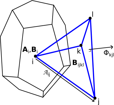
$\mathbf{A}^{(n)}_{i}\rightarrow\mathcal{A}_{ij}\rightarrow\Phi_{ijk}\rightarrow\mathbf{B}_{ijkl}\rightarrow\mathbf{B}^{(n)}_{i}\rightarrow\mathbf{A}^{(n+1)}_{i}$

Figure 1: A geometric representation of the magnetic field quantities used for the unstaggered CT representation on an unstructured mesh. The Voronoi cell $i$ is represented by the polyhedron, and one of the touching Delaunay tetrahedra is shown in blue. Points $i$, $j$, $k$, and $l$ are mesh generating points. Our method evolves the volume-averaged magnetic vector potential, which is projected along Delaunay edges, and used to recover the Delaunay face-averaged magnetic fluxes, Delaunay volume-averaged magnetic fields, and consequently cell-centred magnetic fields. The arrowed diagram shows the order of steps taken to recover the magnetic fields and evolve the system to the next time step.

	moving CT	static CT	moving Powell
$B$       $t=2.0$       $N=16^{3}$
$B$       $t=2.0$       $N=64^{3}$

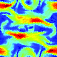
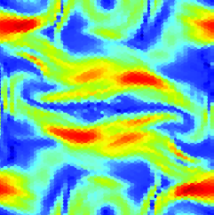
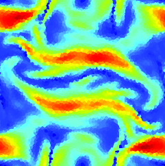
Figure 2: A comparison of moving CT, static CT, and moving Powell schemes for the Orszag-Tang test, as labeled at the top. The magnetic field strength is shown at $t=2.0$, simulated at low (upper panels) and high (lower panels) resolutions. All approaches give results consistent and accurate results.

	moving CT		moving Powell
$t=2\tau_{\rm eddy}$
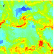
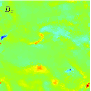
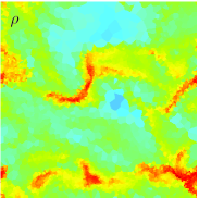
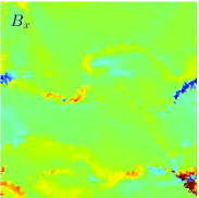
		$\langle\mathbf{B}\rangle=[-0.01,0.01,0.97]$		$\langle\mathbf{B}\rangle=[0.06,0.05,1.21]$
$t=10\tau_{\rm eddy}$
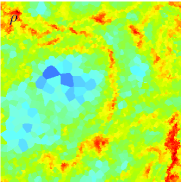
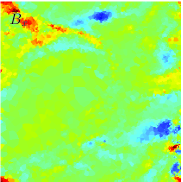
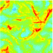
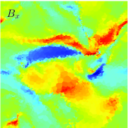
		$\langle\mathbf{B}\rangle=[0.01,0.00,0.99]$		$\langle\mathbf{B}\rangle=[0.59,1.46,3.46]$
$t=40\tau_{\rm eddy}$
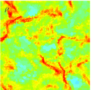
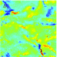
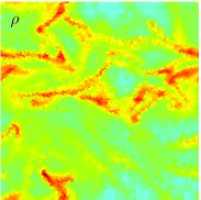
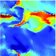
		$\langle\mathbf{B}\rangle=[-0.01,-0.01,0.99]$		$\langle\mathbf{B}\rangle=[-2.78,7.63,6.36]$

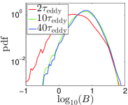
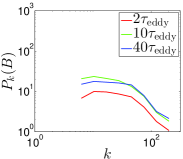
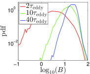
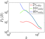
Figure 3: Comparison of the moving mesh CT and Powell schemes used to simulate $\mathcal{M}_{\rm s}\sim 10$, $\mathcal{M}_{\rm A}\sim 3$ turbulence. Plotted are slices of the density field, $x$ component of the magnetic field, and the the PDF and power spectra of the magnetic field at $t=2,10,40$ eddy turnover times. In the plots of $B_{x}$ we also list the volume-averaged mean magnetic field in the domain, which is an ideal MHD invariant (its initial value was set to $\mathbf{B}=(0,0,1)$). At $2$ eddy turnover times, when the turbulence is transitioning into the non-linear saturated regime, the two schemes show similar features in the density and magnetic field. However, after more eddy turnovers, the Powell scheme artificially makes the mean magnetic field grow significantly due to its non-conservative formulation and shifts the entire magnetic field PDF of the magnetic field to the right, as well as transfers most of the magnetic energy to the largest scale ($k=2\cdot\pi$). The CT scheme offers good control over the mean magnetic field and shows a stable PDF and power spectrum of the magnetic field.

moving CT	moving Powell

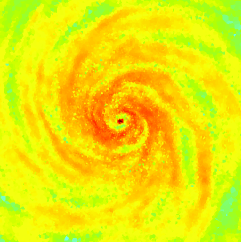
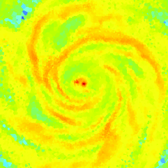
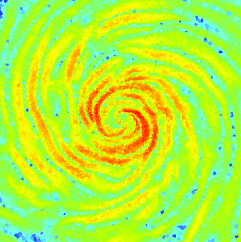
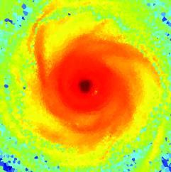
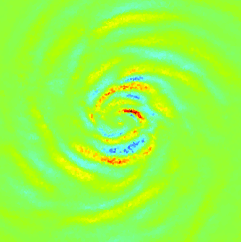
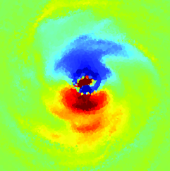
Figure 4: Comparison of magnetic field saturation in the formation of a disc simulated with the CT and Powell schemes. Shown are the density, magnetic field strength, and magnetic field $x$ component, of the disc at $t=2.5$ Gyr. Each panel displays a physical region of side length $40~{}{\rm kpc}$. With the Powell scheme, unlike the CT method, the magnetic field has grown dynamically dominant and disrupts the disc.

The CT mapping is as follows. Define the modified Delaunay tetrahedralization, by which we mean the tetrahedralization obtained from the Delaunay connections, but with the nodes, originally located at the mesh generating points, shifted slightly to the centres-of-mass of the cells. We will refer to the tetrahedra in this tetrahedralization as Delaunay tetrahedra but note that their nodes are slightly offset from the standard definition. Using the centres-of-mass instead of the mesh generating points is formally more accurate for our scheme, but the method may be implemented using the mesh generating points instead, with little effect on the results on a well-regularized mesh.

[1] First, the components $\mathbf{A}_{i}$ are projected onto each of the connections in a modified Delaunay tetrahedralization of the mesh. That is, we obtain

$$\mathcal{A}_{ij}=\mathbf{A}_{i}\cdot d\mathbf{r}_{ij}$$ (9)

where $\mathbf{r}_{ij}$ is the connection pointing from the center-of-mass of cell $i$ to the center-of-mass of cell $j$.

[2] Next, the outward normal component of the magnetic flux $\Phi_{ijk}$ is computed on each of the Delaunay tetrahedral faces (with vertices labelled by mesh generating point $i$, $j$, and $k$). We note that in an unstaggered CT approach, such as that of Mocz, Vogelsberger & Hernquist (2014), the quantities $\Phi_{ijk}$ would be evolved directly. However, evolving the vector potential instead and mapping down to face fluxes is more efficient and easier to implement. The $\Phi_{ijk}$ pointing along the direction given by the right-hand rule with nodes $i$, $j$, and $k$ counter-clockwise, is:

$$\Phi_{ijk}=\frac{1}{2}\left(\mathcal{A}_{ij}-\mathcal{A}_{ji}+\mathcal{A}_{jk}-\mathcal{A}_{kj}+\mathcal{A}_{ki}-\mathcal{A}_{ik}\right)$$ (10)

as it comes from the equation for the magnetic flux through a surface

$$\Phi_{S}=\oint_{\partial S}\mathbf{A}\cdot d\mathbf{\ell}$$ (11)

where the line integral is computed with a counter-clockwise orientation around the boundary of the surface $S$.

[3] Next, the full magnetic field $\mathbf{B}_{ijkl}$ in each Delaunay tetrahedron is reconstructed from the magnetic fluxes $\Phi_{ijk}$, $\Phi_{ijl}$, $\Phi_{jkl}$, $\Phi_{kil}$. Note that the divergence free condition implies $\Phi_{ijk}+\Phi_{ijl}+\Phi_{jkl}+\Phi_{kil}=0$ (it is exactly this value that is preserved to machine precision by our CT approach). So there are $3$ degrees of freedom represented in both $\mathbf{B}_{ijkl}$ and the face magnetic fluxes. Hence, there is a unique magnetic field vector that projects onto the faces to give the four desired (divergence-free) fluxes. We find the value of the magnetic field by inverting the linear system

$$\begin{pmatrix}\mathscr{A}_{x,ijk}\,\mathscr{A}_{y,ijk}\,\mathscr{A}_{z,ijk}\\ \mathscr{A}_{x,ijl}\,\mathscr{A}_{y,ijl}\,\mathscr{A}_{z,ijl}\\ \mathscr{A}_{x,jkl}\,\mathscr{A}_{y,jkl}\,\mathscr{A}_{z,jkl}\end{pmatrix}\begin{pmatrix}B_{x,ijkl}\\ B_{y,ijkl}\\ B_{z,ijkl}\end{pmatrix}=\begin{pmatrix}\Phi_{ijk}\\ \Phi_{ijl}\\ \Phi_{jkl}\\ \end{pmatrix}$$ (12)

where the $\mathbf{\mathscr{A}}_{ijk}$ are the outward vector areas of the faces. Note that we are using an integral condition to recover $\mathbf{B}=\nabla\times\mathbf{A}$, so we are not assuming that $\mathbf{A}$ is differentiable, which can be a pitfall for some vector potential numerical schemes for solving the MHD equations.

[4] Finally, the Delaunay tetrahedral magnetic fields are converted to Voronoi cell magnetic fields $\mathbf{B}_{i}$ by volume averaging all the magnetic fields of the tetrahedra that touch cell $i$.

Fig. 1 illustrates the geometrically-averaged quantities we have defined, and shows a diagram illustrating the steps required to recover the cell-centred magnetic fields.

We also note that a magnetic field needs to be supplied to the Riemann solver for the update of the other fluid variables using the finite volume approach. We found it sufficient to take the extrapolated cell-centred magnetic fields out to the faces, with the normal component through the face averaged across the two sides, as done in Pakmor, Bauer & Springel (2011).

2.3 Magnetic vector potential in periodic boundary conditions

Here we describe the implementation of the magnetic vector potential approach in a periodic domain. Note that while $\mathbf{B}$ is periodic, $\mathbf{A}=\nabla\times\mathbf{B}$ need not be. However, in general, the magnetic vector potential may be decomposed into a periodic part and a non-periodic part which corresponds to the mean magnetic field, which is an invariant of ideal MHD. Thus:

$$\mathbf{A}_{i}(\mathbf{x},t)=\mathbf{A}_{i,\textrm{mean-field}}(\mathbf{x})+\mathbf{A}_{i,\textrm{periodic}}(\mathbf{x},t)$$ (13)

So, to implement periodic boundary conditions, one may keep track of and update $\mathbf{A}_{i,\textrm{periodic}}(\mathbf{x},t)$ and always add to it $\mathbf{A}_{i,\textrm{mean-field}}(\mathbf{x})$, which is static in time and determined by the mean-field.

3 Numerical Tests

We test our numerical method on five problems: the classic Orszag-Tang vortex, the propagation of a circularly polarized Alfvén wave, driven MHD turbulence, the formation of an idealized magnetized disc, and a cosmological volume with stellar and black hole feedback.

3.1 Orszag-Tang

First, we compare our moving mesh CT method to CT on a static mesh and moving-mesh Powell cleaning by simulating the classic Orszag & Tang (1979) vortex, a well-known 2D test problem for MHD codes that initiates decaying supersonic turbulence. Our set-up of the problem is described in Mocz, Vogelsberger & Hernquist (2014). Here, we simulate this 2D system inside a 3D box, with all fluid variables being repeated along the $z$-direction. The initial mesh generating points are staggered, to yield a non-degenerate Delaunay tetrahedralization of the mesh (which is not necessary for our method, but speeds up initial mesh construction). We simulate the system using resolutions of $N=16^{3}$ and $N=64^{3}$ to evaluate the pre-converged and resolved behaviours of the methods.

Fig. 2 shows the results of the tests. All the methods give robust, accurate answers with sufficient resolution. We used an initially staggered mesh that is not exactly aligned with the symmetries of the initial conditions, hence giving rise to small asymmetries in all the simulations. At low/marginally-resolved resolution, the Powell scheme can be sensitive to the divergence-cleaning source term, since divergence errors can be the largest at low resolution, which breaks the symmetry of the problem to a greater extent.

3.2 Circularly-polarized Alfvén wave

We simulate the circularly-polarized Alfvén wave of Tóth (2000) in 3D. The solution has a known analytic expression, and therefore we can use this test to verify the convergence properties of our scheme. The non-linear Alfvén wave is chosen to propagate along the diagonal of a $2\times 1\times 1$ periodic box of size $3\times 1.5\times 1.5$, as described in Stone et al. (2008). We use a staggered mesh with resolution $2\times(2N\times N\times N)$. The problem is initialized with $\rho=1$, $p_{\rm gas}=0.1$, $\Gamma=5/3$. In a coordinate frame defined along the diagonal, the wave has velocity and magnetic field $v_{\perp}=B_{\perp}=0.1\sin(2\pi x_{\|})$, $v_{\|}=0$, $B_{\|}=1$, $v_{z}=B_{z}=0.1\cos(2\pi x_{\|})$. The solution returns to it’s original state at time $t=1$.

Fig. 5 shows the convergence of the magnetic field of the Alfvén wave at $t=1$ as a function of the resolution $N$. The analysis shows second order behaviour as expected for both the Powell and CT schemes.

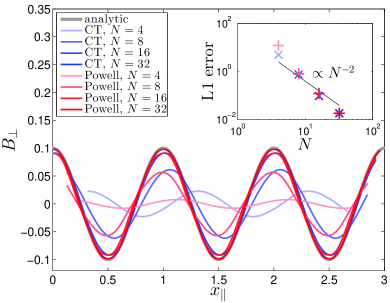
Figure 5: Convergence of the non-linear circularly-polarized Alfvén wave (3D simulation) with the moving Powell and CT schemes.

3.3 Turbulent box

We next simulate isothermal supersonic MHD turbulence using the driving routine of Federrath et al. (2010); Price & Federrath (2010), adapted for the Arepo code in Bauer & Springel (2012). The initial conditions are set up in dimensionless units: boxsize $L=1$, sound speed $c_{s}=1$, initial density $\rho_{0}=1$, initial magnetic field $\mathbf{B}=(0,0,1)$, and we use $64^{3}$ resolution elements. We drive the velocity field solenoidally in Fourier-space on large spatial injection scales to establish a turbulent box characterized by a sonic Mach number of $\mathcal{M}_{\rm s}\sim 10$ and Alfvénic Mach number of $\mathcal{M}_{\rm s}\sim 3$. Saturated turbulence (i.e., with steady time-averaged statistical properties modulo the effects of intermittency) is expected to be established after a few eddy turnover times.

The results of our simulation are shown in Fig. 3. We plot a slice of the density field, $x$-direction magnetic field, probability density function (PDF) of the magnetic field strength, and the radially averaged $1D$ power spectrum of the magnetic field at $2$, $10$, and $40$ eddy turnover times. At $2$ eddy turnover times, when the turbulence is transitioning into the non-linear saturated regime, both the CT and Powell scheme show similar features in the density and magnetic field, and the power spectrum (we have used the same random number seed for the turbulent driving). Hence, we know that both codes perform reasonably well in the linear regime of this simulation. The magnetic field power-spectrum is flat on the injection scales and falls over the inertial range. This shape is in good agreement with the magnetic power spectra calculated in Tricco, Price & Federrath (2016), which compares turbulent box simulations using a Cartesian mesh constrained transport scheme (implemented in FLASH) and an SPH method for MHD.

At later times, the CT and Powell schemes differ. The CT scheme shows approximately time-steady behaviour of the magnetic field PDF and power spectrum, as expected. Additionally, the volume averaged mean magnetic field ($\langle\mathbf{B}\rangle=(0,0,1)$), a conserved quantity in ideal MHD, is well-preserved. Fig. 3 lists the mean field values, which are generally preserved to within $1$ per cent (in fact, they are conserved to machine precision under our scheme on a static mesh, as is the case for the original CT scheme). The Powell scheme, on the other hand, shows poor behaviour in the non-linear regime. The mean magnetic field continues to grow, the magnetic field PDF keeps shifting to the right to higher field strengths, and power is transferred to the largest spatial scale ($k=2\cdot\pi$). The magnetic field have grown by over an order-of-magnitude from its expected value. This is problematic for the simulation: the magnetic field becomes dominant and changes the nature of the turbulence as it transitions from a super-Alfvénic to sub-Alfvénic regime.

moving CT	moving Powell

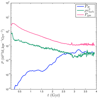
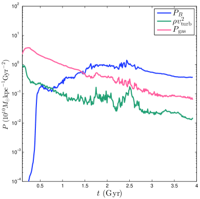
Figure 6: Comparison of magnetic field saturation in the formation of a disc simulated with the CT and Powell schemes. The CT method shows equipartition between magnetic energy density and turbulent kinetic energy density, whereas the Powell technique saturates the field at higher values, exceeding the thermal pressure by about a factor of five.

moving CT	moving Powell

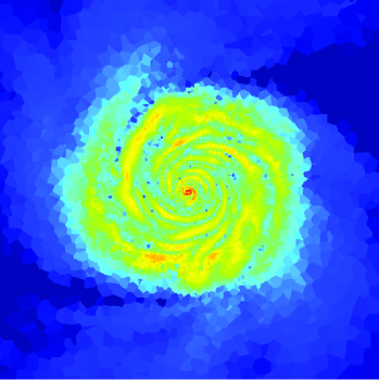
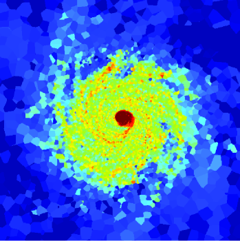
Figure 7: Comparison of the magnetic field strength of the same disc in Fig. 4 at time $t=0.5~{}{\rm Gyr}$ in the formation process, simulated using the CT and Powell schemes. The figure displays a physical size of $40~{}{\rm kpc}$. The CT approach exhibits much better preservation of the topological winding of the magnetic field. The Powell scheme shows substantial divergence error noise seen on the cell level while this is absent to machine precision in CT.

moving CT	moving Powell

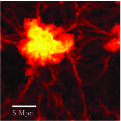
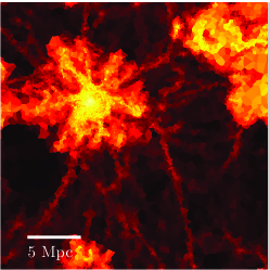
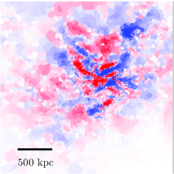
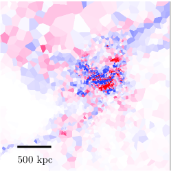
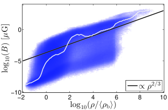
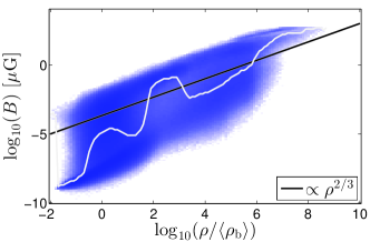
Figure 8: Magnetic fields (strength and $x$-component, top and middle panels respectively) and their phase-space distribution (bottom panels) at $z=0$, in a $h^{-1}25~{}{\rm Mpc}$ cosmological box with full feedback physics as obtained with the CT and Powell schemes. The magnetic strengths and the phase space diagram are similar. In the phase-space diagram, the white line shows the median magnetic field strength at a given density. Under pure adiabatic compression, $B\propto\rho^{2/3}$ is expected due to flux-freezing. There is a difference in the magnetic field topology in the two simulations. The zoom-in on the $B_{x}$ profile shows that the CT scheme exhibits larger structure and less individual cell-scale noise.

3.4 Magnetic Disc

We simulate the formation of an isolated Milky-Way sized disc galaxy under idealized conditions, as done previously in Pakmor & Springel (2013), which used the moving Powell method to evolve the magnetic fields. Here, we compare results from the moving CT and moving Powell methods. Our simulation set-up uses $2\cdot 10^{5}$ particles (effective mass resolution of $\sim 3\times 10^{5}~{}M_{\odot}$), and has an initial $3\cdot 10^{-10}~{}{\rm G}$ magnetic field along the $x$-axis. The total angular momentum vector is initially along the $z$-axis.

The results comparing our CT method with the Powell cleaning are given in Figs. 4 and 6. We show the density field, magnetic field strength, and $x$ component of the magnetic field in the disc at $2.5$ Gyr in Fig. 4. We show the time evolution of the magnetic pressure, thermal pressure, and turbulent kinetic energy density in Fig. 6. These quantities are calculated as volume averaged values inside a cylinder of radius $15~{}{\rm kpc}$ and height $1~{}{\rm kpc}$ centred on the disc. The turbulent velocity for the calculation of the turbulent kinetic energy density is calculated by subtracting the mean rotational velocity (the formed disc has a flat $\sim 200~{}{\rm km}~{}{\rm s}^{-1}$ rotation curve) from the gas velocities and computing the root-mean-square.

Using the Powell scheme, Pakmor & Springel (2013) found that the magnetic field strength in the disc is quickly amplified, due to small-scale dynamo action, shearing motions and the central starburst, and eventually saturates. In this equilibrium state, the magnetic field pressure equals a few times the thermal pressure.

Our results with the CT scheme provide a modified picture. The saturation proceeds more slowly and reaches a lower value. This asymptotic level is in equipartition with the turbulent kinetic energy density, in agreement with the theoretical and numerical understanding of the galactic dynamo and turbulence as well as observations of our Galaxy (Kraichnan, 1965; Zweibel & McKee, 1995; Beck et al., 1996; Hawley, Gammie & Balbus, 1996). The topology of the magnetic field is also quite different. The winding structure of the magnetic field is preserved to a greater degree with CT. The magnetic field in the CT method is not dynamically large enough to disrupt the central parts of the disc and cause strong outflows for our particular set-up. The winding of the magnetic field is expected, as the divergence-free condition enforces a topological constraint on the magnetic field. The ability of a CT code as opposed to Powell cleaning to maintain topological constraints is shown in Fig. 7, where we plot the magnetic field structure in the disc at a time of $0.5~{}{\rm Gyr}$ before much of the magnetic field amplification due to shear and small-scale dynamo action has taken place (thus we would expect a smooth profile showing twisting of the field lines that follows the rotation of the fluid). We see clearly that the CT algorithm exhibits a winding-structure of the magnetic field whereas the Powell scheme has considerable noise at the level of individual mesh cells due to divergence errors. We have quantified the divergence errors relative to the total gas pressure, which describes the dynamical effects of the error. With the CT scheme, the divergence errors are zero to the level of machine precision, while in the Powell scheme, we have found that the errors are of order $10$ percent in the central parts of the disc.

3.5 Cosmological Box

We simulate a $25h^{-1}~{}{\rm Mpc}$ box cosmological box at $256^{3}$ resolution with a weak initial seed magnetic field of strength $10^{-14}~{}{\rm G}$, using the set-up described in Marinacci et al. (2015). The simulation includes the full physics (stellar and active-galactic nuclei (AGN) feedback and radiative cooling) of the Illustris simulation (Vogelsberger et al., 2013, 2014a, 2014b; Nelson et al., 2015). Fig. 8 shows the $z=0$ magnetic field strength in a slice of the box, the magnetic field $B_{x}$ component zoomed in on a halo, and $\rho$–$B$ phase-space distribution of the gas. The phase-space distribution of the magnetic field strengths and the densities (normalized by mean baryon density) are fairly similar for the CT and Powell methods. The phase-space distribution is expected to follow a $B\propto\rho^{2/3}$ under pure adiabatic compression due to the flux-freezing condition (solid black line). The magnetic field exceeds this value due to amplification by shearing and dynamo action. Federrath et al. (2011b) isolate the dynamo action and separating it from the compressional amplification of B, and provide general properties of the dynamo in a compressible gas in Federrath et al. (2011a). Only in halo centres does the magnetic field become strong enough to slightly influence the gas dynamics. While magnetic fields are amplified to similar strengths using the two numerical methods, their topologies differ. The Powell scheme shows more noise at the level of individual cells due to divergence errors. Some of the differences in the structure is attributed to the stochasticity of the feedback model.

3.5.1 Induction equation in comoving coordinates

We offer remarks on how we chose to implement the induction equation in cosmological comoving coordinates. The global expansion of the universe is characterized by the time-dependent scale factor $a(t)$. The simulation is evolved on a mesh in comoving variables $\mathbf{x}$, and the standard physical fluid variables are also converted to ‘comoving’ variables, which are the quantities being evolved. We use the quantities defined in section 2.2 of Pakmor & Springel (2013). The ‘comoving’ magnetic field $\mathbf{B}_{\rm c}$ that our base scheme solves is related to the physical magnetic field $\mathbf{B}$ by $\mathbf{B}=\mathbf{B}_{\rm c}a^{-2}$. As Pakmor & Springel (2013) point out, this choice has the advantage of eliminating source terms in the induction equation. For our vector potential CT scheme, we define the ‘comoving’ vector potential $\mathbf{A}_{\rm c}$ by $\mathbf{B}_{\rm c}=\nabla_{\mathbf{x}}\times\mathbf{A}_{\rm c}$. The induction equation is then given by:

$$\frac{\partial\mathbf{A}_{\rm c}}{\partial t}=-\frac{1}{a}\left(-\mathbf{u}\times\mathbf{B}_{\rm c}\right)$$ (14)

where $\mathbf{u}$ is the peculiar velocity.

4 Discussion

While the Powell and CT schemes both yield accurate results in idealized test problems (such as the Orszag-Tang vortex and the propagation of a circularly polarized Alfvén wave), we find that the two approaches can lead to different outcomes for astrophysical flows with magnetic field amplification and turbulence in the non-linear regime. Divergence cleaning techniques have been shown to produce spurious structures and magnetic energy fluctuations on small spatial scales due to the non-locality of the cleaning step (Tóth, 2000; Balsara & Kim, 2004), whereas CT schemes produce robust results.

In moving mesh simulations of turbulent and astrophysical flows, the Powell and CT schemes give a similar general picture, but exhibit some quantitative differences. Zhu et al. (2015) discusses that Powell cleaning gives faster field growth and larger saturation at lower resolutions in general, where the divergence errors are larger. This is consistent with our results for the magnetized disc. The CT method reaches the natural equipartition between the magnetic energy density and the turbulent kinetic energy density in the disc, whereas the Powell scheme overshoots this value and the magnetic pressure dominates the gas pressure by a factor of five. In the original Powell magnetic disc simulations of Pakmor & Springel (2013), the authors find even larger ($>10\times$) overshoots of the magnetic pressure over gas pressure in their lowest resolution simulation ($12500$ particles; see their Figure 7). The CT scheme can be considered particularly more robust at low/marginally-resolved resolutions, which will always be the situation in practice for some structures in large-scale cosmological simulations.

This difference between CT and Powell in the growth rate and saturation of the magnetic field in magnetized disc galaxies is observed across different codes in the literature as well. Adaptive mesh refinement (AMR) with the divergence-preserving CT scheme (Wang & Abel, 2009; Dubois & Teyssier, 2010; Rieder & Teyssier, 2016) find slow growth rates compared to the fast growth rates (e-folding time $\sim 10$ Myr) of divergence cleaning schemes implemented in SPH (Beck et al., 2012) or moving mesh (Pakmor & Springel, 2013). The difference we observe between our CT and Powell simulations suggests that divergence cleaning, and not the Eulerian vs Lagrangian natures of the codes, is the culprit. Rieder & Teyssier (2016) point out that in simulations without strong stellar feedback (such as ours), the flows are relatively smooth and two-dimensional, a regime in which strong dynamo amplification is difficult.

In the case of the cosmological box simulations, the two schemes give similar statistics for the overall magnetic field strengths in the density - magnetic field phase space. However, the CT algorithm produces a smoother magnetic field, without the magnetic field unphysically flipping at the single-cell level. This property will improve Faraday rotation measure estimates and cosmic ray propagation (Pfrommer et al., 2016; Pakmor et al., 2016a) in the Arepo code.

The difference between the moving mesh CT and Powell schemes can perhaps be best understood with the idealized turbulence test, where the behaviour of the true solution is known theoretically. The Powell scheme, with its non-conservative formulation (divergence correcting source-terms), artificially makes the magnetic field grow in this particular test problem and quickly transfers magnetic energy to the largest scales. The mean magnetic field (which should be a conserved quantity in ideal MHD as the equations for the evolution of the magnetic field can be recast into standard conservative hyperbolic form) grows by over an order of magnitude and information about the initial mean field direction is also lost. Interestingly, the disc simulation shows similar difference between the CT and Powell schemes as these turbulence tests; namely the Powell scheme grows the magnetic field beyond the turbulent kinetic energy and most of the magnetic power is on the largest scales (size of the disc).

Finally, we also note that our unstructured (cell-centred) CT formalism may find useful application in static mesh codes, and may potentially be used to simplify some of the technical details of implementing CT in a code with AMR (Balsara, 2001; Fromang, Hennebelle & Teyssier, 2006; Mignone et al., 2012) as well.

A moving mesh unstaggered CT approach has some practical advantages over an AMR code with staggered CT. The unstaggered representation allows for straightforward coupling with refinement and power of two hierarchical time stepping on a moving Voronoi mesh. There is no difficulty introduced as in the fine and coarse level mismatch in AMR codes, where specific care (such as restriction, prolongation, and reflux-curl operations Miniati & Martin 2011) has to be taken to prevent a loss of order of accuracy and breaking of the divergence-free condition at interface regions. In addition, the moving mesh approach provides the usual advantages of automatic adaptivity and reduced advection errors.

Summarizing, we have developed an efficient, accurate, unstructured CT scheme for solving the MHD equations in 3D on a moving mesh. The CT formulation allows for the maintenance of the divergence-free condition on the magnetic field to machine precision, which leads to numerical stability, more accurate numerical solutions, and good preservation of the topological properties of the magnetic field. The numerical experiments we considered demonstrate the advantages of CT schemes over cleaning schemes, namely preventing artificial magnetic field growth due to the source terms in cleaning schemes. The new CT method, implemented in the moving mesh code Arepo, will allow for powerful MHD simulations in the upcoming future, making use of the advantages of an adaptive, quasi-Lagrangian treatment of the fluid equations.

Appendix A Other gauge choices

The evolution of the magnetic field is invariant under a choice of gauge $\psi$ for the vector potential:

$$\frac{\partial\mathbf{A}}{\partial t}=-\mathbf{E}-\nabla\psi$$ (15)

In the present work, we chose to evolve the vector potential under the Weyl gauge ($\psi=0$), as it offers a nice correspondence between CT and vector potential methods because one is adding just the same EMF terms to update the solution in both cases. However, it may be of some interest to explore other gauge choices in future work, as they can be more suitable to the treatment of particular problems/physical processes. We briefly discuss alternate choices here.

One may choose the Coulomb gauge, $\nabla\cdot\mathbf{A}=0$. This gauge choice would require using either projection methods or cleaning methods on $\mathbf{A}$ to keep it divergence free. This choice of gauge would simplify the extension of the ideal MHD code to resistive MHD, as the induction equation for resistive MHD is given by:

$$\frac{\partial\mathbf{A}}{\partial t}=\mathbf{v}\times\mathbf{B}-\eta\nabla\times(\nabla\times\mathbf{A})$$ (16)

where the resistive term expands as: $\eta\nabla(\nabla\cdot\mathbf{A})-\eta\nabla^{2}\mathbf{A}$, which is just a diffusion term if $\nabla\cdot\mathbf{A}=0$.

Another choice would be to choose a helicity-like gauge: $\psi=\mathbf{v}\cdot\mathbf{A}$. This choice of gauge makes the magnetic vector potential induction equation Galilean-invariant:

$$\frac{d\mathbf{A}}{dt}=-\mathbf{A}\times\nabla\times\mathbf{v}-(\mathbf{A}\cdot\nabla)\mathbf{v}=-\boldsymbol{J}_{\mathbf{v}}^{\rm T}\mathbf{A}$$ (17)

where $\boldsymbol{J}_{\mathbf{v}}$ denotes the Jacobian of $\mathbf{v}$. The downside of this gauge is that the velocity field may not be differentiable, so special care would have to be taken for the treatment of the Jacobian term in the presence of shocks.

A final interesting choice would be to modify the above helicity-like gauge to use the mesh motion velocity $\mathbf{w}$ instead: $\psi=\mathbf{w}\cdot\mathbf{A}$, in which case the induction equation becomes

$$\frac{d\mathbf{A}}{dt}=(\mathbf{v}-\mathbf{w})\times\mathbf{B}-\boldsymbol{J}_{\mathbf{w}}^{\rm T}\mathbf{A}$$ (18)

The first term $(\mathbf{v}-\mathbf{w})\times\mathbf{B}$ is just the electric field in the frame of the moving mesh, which is $0$ if the mesh cell moves exactly with the fluid. This choice of gauge reduces to the Weyl gauge in the case of a static mesh. Such a gauge would require smoothed mesh motion (e.g. Duffell & MacFadyen 2015) to treat the Jacobian term accurately and avoid mesh noise.

References

- Balsara (2001) Balsara D. S., 2001, Journal of Computational Physics, 174, 614
- Balsara & Kim (2004) Balsara D. S., Kim J., 2004, ApJ, 602, 1079
- Balsara & Spicer (1999) Balsara D. S., Spicer D. S., 1999, Journal of Computational Physics, 149, 270
- Bauer & Springel (2012) Bauer A., Springel V., 2012, MNRAS, 423, 2558
- Beck et al. (2012) Beck A. M., Lesch H., Dolag K., Kotarba H., Geng A., Stasyszyn F. A., 2012, MNRAS, 422, 2152
- Beck et al. (1996) Beck R., Brandenburg A., Moss D., Shukurov A., Sokoloff D., 1996, ARA&A, 34, 155
- Collins et al. (2012) Collins D. C., Kritsuk A. G., Padoan P., Li H., Xu H., Ustyugov S. D., Norman M. L., 2012, ApJ, 750, 13
- Dedner et al. (2002) Dedner A., Kemm F., Kröner D., Munz C.-D., Schnitzer T., Wesenberg M., 2002, Journal of Computational Physics, 175, 645
- Dubois & Teyssier (2010) Dubois Y., Teyssier R., 2010, A&A, 523, A72
- Duffell & MacFadyen (2011) Duffell P. C., MacFadyen A. I., 2011, ApJS, 197, 15
- Duffell & MacFadyen (2015) —, 2015, MNRAS, 449, 2718
- Evans & Hawley (1988) Evans C. R., Hawley J. F., 1988, ApJ, 332, 659
- Federrath (2015) Federrath C., 2015, MNRAS, 450, 4035
- Federrath et al. (2011a) Federrath C., Chabrier G., Schober J., Banerjee R., Klessen R. S., Schleicher D. R. G., 2011a, Physical Review Letters, 107, 114504
- Federrath & Klessen (2012) Federrath C., Klessen R. S., 2012, ApJ, 761, 156
- Federrath et al. (2010) Federrath C., Roman-Duval J., Klessen R. S., Schmidt W., Mac Low M.-M., 2010, A&A, 512, A81
- Federrath et al. (2011b) Federrath C., Sur S., Schleicher D. R. G., Banerjee R., Klessen R. S., 2011b, ApJ, 731, 62
- Fromang, Hennebelle & Teyssier (2006) Fromang S., Hennebelle P., Teyssier R., 2006, A&A, 457, 371
- Gaburov, Johansen & Levin (2012) Gaburov E., Johansen A., Levin Y., 2012, ApJ, 758, 103
- Hawley, Gammie & Balbus (1996) Hawley J. F., Gammie C. F., Balbus S. A., 1996, ApJ, 464, 690
- Hopkins (2015) Hopkins P. F., 2015, MNRAS, 450, 53
- Hopkins & Raives (2016) Hopkins P. F., Raives M. J., 2016, MNRAS, 455, 51
- Kelley, Tchekhovskoy & Narayan (2014) Kelley L. Z., Tchekhovskoy A., Narayan R., 2014, MNRAS, 445, 3919
- Kraichnan (1965) Kraichnan R. H., 1965, Physics of Fluids, 8, 1385
- Marinacci & Vogelsberger (2016) Marinacci F., Vogelsberger M., 2016, MNRAS, 456, L69
- Marinacci et al. (2015) Marinacci F., Vogelsberger M., Mocz P., Pakmor R., 2015, MNRAS, 453, 3999
- McCourt et al. (2012) McCourt M., Sharma P., Quataert E., Parrish I. J., 2012, MNRAS, 419, 3319
- McKinney et al. (2014) McKinney J. C., Tchekhovskoy A., Sadowski A., Narayan R., 2014, MNRAS, 441, 3177
- Mignone et al. (2012) Mignone A., Zanni C., Tzeferacos P., van Straalen B., Colella P., Bodo G., 2012, ApJS, 198, 7
- Miniati & Martin (2011) Miniati F., Martin D. F., 2011, ApJS, 195, 5
- Mocz, Vogelsberger & Hernquist (2014) Mocz P., Vogelsberger M., Hernquist L., 2014, MNRAS, 442, 43
- Myers et al. (2013) Myers A. T., McKee C. F., Cunningham A. J., Klein R. I., Krumholz M. R., 2013, ApJ, 766, 97
- Nelson et al. (2015) Nelson D. et al., 2015, Astronomy and Computing, 13, 12
- Orszag & Tang (1979) Orszag S. A., Tang C.-M., 1979, Journal of Fluid Mechanics, 90, 129
- Pakmor, Bauer & Springel (2011) Pakmor R., Bauer A., Springel V., 2011, MNRAS, 418, 1392
- Pakmor, Marinacci & Springel (2014) Pakmor R., Marinacci F., Springel V., 2014, ApJ, 783, L20
- Pakmor et al. (2016a) Pakmor R., Pfrommer C., Simpson C. M., Springel V., 2016a, ArXiv e-prints 1605.00643
- Pakmor & Springel (2013) Pakmor R., Springel V., 2013, MNRAS, 432, 176
- Pakmor et al. (2016b) Pakmor R., Springel V., Bauer A., Mocz P., Munoz D. J., Ohlmann S. T., Schaal K., Zhu C., 2016b, MNRAS, 455, 1134
- Pfrommer et al. (2016) Pfrommer C., Pakmor R., Schaal K., Simpson C. M., Springel V., 2016, ArXiv e-prints 1604.07399
- Powell et al. (1999) Powell K. G., Roe P. L., Linde T. J., Gombosi T. I., De Zeeuw D. L., 1999, Journal of Computational Physics, 154, 284
- Price & Federrath (2010) Price D. J., Federrath C., 2010, MNRAS, 406, 1659
- Rieder & Teyssier (2016) Rieder M., Teyssier R., 2016, MNRAS, 457, 1722
- Sa̧dowski et al. (2014) Sa̧dowski A., Narayan R., McKinney J. C., Tchekhovskoy A., 2014, MNRAS, 439, 503
- Springel (2010) Springel V., 2010, MNRAS, 401, 791
- Stone et al. (2008) Stone J. M., Gardiner T. A., Teuben P., Hawley J. F., Simon J. B., 2008, ApJS, 178, 137
- Tóth (2000) Tóth G., 2000, Journal of Computational Physics, 161, 605
- Tricco (2015) Tricco T. S., 2015, ArXiv e-prints 1505.04494
- Tricco, Price & Federrath (2016) Tricco T. S., Price D. J., Federrath C., 2016, ArXiv e-prints 1605.08662
- Vogelsberger et al. (2013) Vogelsberger M., Genel S., Sijacki D., Torrey P., Springel V., Hernquist L., 2013, MNRAS, 436, 3031
- Vogelsberger et al. (2014a) Vogelsberger M. et al., 2014a, Nat, 509, 177
- Vogelsberger et al. (2014b) —, 2014b, MNRAS, 444, 1518
- Wang & Abel (2009) Wang P., Abel T., 2009, ApJ, 696, 96
- Yee (1966) Yee K., 1966, IEEE Transactions on Antennas and Propagation, 14, 302
- Zhu et al. (2015) Zhu C., Pakmor R., van Kerkwijk M. H., Chang P., 2015, ApJ, 806, L1
- Zweibel & McKee (1995) Zweibel E. G., McKee C. F., 1995, ApJ, 439, 779