On the nature of hydrostatic equilibrium in galaxy clusters

Abstract

In this paper we investigate the level of hydrostatic equilibrium (HE) in the intra-cluster medium of simulated galaxy clusters, extracted from state-of-the-art cosmological hydrodynamical simulations performed with the Smoothed-Particle-Hydrodynamic code GADGET-3. These simulations include several physical processes, among which stellar and AGN feedback, and have been performed with an improved version of the code that allows for a better description of hydrodynamical instabilities and gas mixing processes. Evaluating the radial balance between the gravitational and hydrodynamical forces, via the gas accelerations generated, we effectively examine the level of HE in every object of the sample, its dependence on the radial distance from the center and on the classification of the cluster in terms of either cool-coreness or dynamical state. We find an average deviation of 10–20% out to the virial radius, with no evident distinction between cool-core and non-cool-core clusters. Instead, we observe a clear separation between regular and disturbed systems, with a more significant deviation from HE for the disturbed objects. The investigation of the bias between the hydrostatic estimate and the total gravitating mass indicates that, on average, this traces very well the deviation from HE, even though individual cases show a more complex picture. Typically, in the radial ranges where mass bias and deviation from HE are substantially different, the gas is characterized by a significant amount of random motions ($\gtrsim 30$ per cent), relative to thermal ones. As a general result, the HE-deviation and mass bias, at given interesting distance from the cluster center, are not very sensitive to the temperature inhomogeneities in the gas.

1 Introduction

As fair samples of the Universe, galaxy clusters are dominated in mass, $\sim 80$ per cent, by dark matter (DM) but also comprise a significant amount of baryonic visible matter, in the form of galaxies and hot plasma ($\sim 5$ and $\sim 15$ per cent in mass, respectively). In the accepted scenario of hierarchical structure formation, clusters grow via smooth accretion processes as well as through merger events (see Kravtsov & Borgani, 2012, for a review). According to this theoretical framework, the hot intra-cluster medium (ICM) is assumed to collapse within the cluster DM halo, get shock heated during the assembly process, and finally settle with temperatures of order $10^{7}$–$10^{8}$ K, reflecting the depth of the potential well ($\sim 10^{14}$–$10^{15}\rm{\,M_{\odot}}$). The dynamics of the intra-cluster gas can be described by the Euler equation:

$$\frac{d{\bf v}}{dt}=-\nabla\Phi-\frac{1}{\rho}\nabla P\,.$$ (1)

Here, $P$ is the total gas pressure, $\Phi$ is the cluster potential and

$$\frac{d{\bf v}}{dt}=\frac{\partial{\bf v}}{\partial t}+\left({\bf v}\cdot\nabla\right){\bf v}$$ (2)

is the Lagrangian derivative of the velocity or the sum of the acceleration and the inertia terms, respectively the first and second term on the l.h.s. of Eq. 2. The condition of hydrostatic equilibrium (HE) is represented by

$$\frac{d{\bf v}}{dt}=0\,.$$ (3)

This assumption implies that the net Lagrangian three-dimensional acceleration of the gas, resulting from the sum of hydrodynamical and gravitational forces, is null. With our numerical study, we intend to investigate whether the condition expressed by Eq. (3), and so the balance between hydrodynamical and gravitational forces is reliable in cosmological simulations of galaxy clusters, when evaluated at typical, interesting distances from the cluster center. In fact, the assumption of HE is key ingredient behind one of the most diffuse methods employed to measure the galaxy cluster mass, which is the crucial property to characterize a cluster for astrophysical as well as cosmological purposes.

Specifically, the reconstruction of the so-called hydrostatic mass from X-ray observations of the ICM thermal properties can be derived from Eq. (3) re-formulated as

$$0=-\nabla\Phi-\frac{1}{\rho}\nabla P\,,$$

along with the additional assumptions of spherical symmetry and of a purely thermal pressure support of the gas ($P=P_{\rm th}$). Under these conditions, and further assuming the equation of state of an ideal gas to hold for the ICM, one can derive the total mass from the profiles of gas density ($\rho$) and temperature ($T$):

$$M_{\rm HE}(<r)=-\frac{k_{B}T(r)r}{\mu Gm_{p}}\left[\frac{d\log\rho(r)}{d\log r}+\frac{d\log T(r)}{d\log r}\right],$$ (4)

where $k_{B}$ is the Boltzmann constant, $\mu$ the mean molecular weight, $G$ is the gravitational constant, and $m_{p}$ the proton mass.

For regular virialized galaxy clusters the above assumptions are a reasonable representation of the gas state. However, if any of the hypotheses done are not satisfied, the hydrostatic mass might provide a biased estimate of the true gravitating mass.

Observationally, the particular composition of galaxy clusters allows us to observe them in many different wavelengths other than X-rays, such as optical or millimetric bands, providing independent methods to reconstruct their intrinsic structure and total mass (see e.g. Mahdavi et al., 2008, 2013; von der Linden et al., 2014; Sereno & Ettori, 2015; Applegate et al., 2015; Simet et al., 2015; Smith et al., 2016). Some of these approaches, such as the one based on optical observations of the weak lensing effect, are less sensitive to the complex non-gravitational processes that characterise the gas and have been commonly used for comparisons to X-ray mass estimates (e.g. Donahue et al., 2014). A mismatch between optical and X-ray mass measurements has been often interpreted as lack of HE. Nonetheless, it is important to notice that the violation of any of the assumptions behind Eq. (4) can lead to a bias in the mass estimate, even in the presence of a perfect balance between gravity and pressure.

To this end, numerical studies based on state-of-the-art cosmological hydrodynamical simulations of galaxy clusters offer an optimal way of tackling the problem. Several groups have explored the hydrodynamical stability of simulated clusters, computing the thermal and non-thermal components derived from Eqs. (1) and (2) that contribute to the total support against the cluster gravitational potential and, if neglected, induce the hydrostatic mass bias. In fact, hydrodynamical simulations show that a non-negligible fraction of the ICM pressure support is due to turbulent and bulk gas motions, and this should be taken into account for the mass estimation based on hydrostatic equilibrium Rasia et al. (2004); Lau et al. (2009); Fang et al. (2009); Vazza et al. (2009); Biffi et al. (2011); Suto et al. (2013); Lau et al. (2013); Gaspari & Churazov (2013); Gaspari et al. (2014); Nelson et al. (2014). Previous attempts to specifically identify the principal sources of bias led however to different conclusions, mainly because of differences in the terminology, computational method or interpretation of the mass terms involved Suto et al. (2013); Lau et al. (2013); Shi et al. (2015). In Fang et al. (2009) the major source of additional pressure support against gravity has been ascribed to gas rotational patterns, especially in the center of relaxed systems, whilst in Lau et al. (2009) the authors found a significantly higher contribution to the total pressure support coming from random motions. More recently, numerical investigations by Suto et al. (2013) and Nelson et al. (2014) additionally explored the possibility of a non-steady state of the gas, i.e. $\partial{\bf v}/\partial t\neq 0$, in Eq. (2), and assessed the importance of accounting for gas acceleration as well. The common finding of numerical works is that, even for very regular clusters, the hydrostatic mass overall underestimates the true gravitating mass by a typical factor of $10$–$20$ per cent (see e.g. Rasia et al., 2004, 2006; Jeltema et al., 2008; Piffaretti & Valdarnini, 2008; Meneghetti et al., 2010; Nelson et al., 2012). Independently of this, also the presence of gas temperature inhomogeneities can cause an additional bias in the temperature estimate from current X-ray telescopes, thus originating a total difference between X-ray derived and true masses of up to $30$ per cent (e.g., Rasia et al., 2014).

Even if challenging, the detection of gas turbulent and bulk motions will substantially improve with observations from next-generation X-ray calorimeters, on board satellites such as ASTRO-H or Athena. Their unprecedented level of energy resolution will eventually allow us to put tighter constraints on the ICM motions, measuring gas velocities from the broadening and center shifts of heavy-ions emission lines in the X-ray spectra down to few hundreds km/s Biffi et al. (2013); Nandra et al. (2013); Ettori et al. (2013).

Nonetheless, it is very difficult to measure corrections for the mass bias and generally deviations from HE of the gas on a single cluster base at intermediate-high redshift, where the spatial precision is more limited, and a statistical approach is therefore preferable. In fact, a thorough investigation of the origin of HE violation for individual cases can only be pursued via numerical simulations, which grant access to the full three-dimensional thermal and velocity structure of clusters and to their dynamical history. Complementary to this, simulations can also be exploited to provide general predictions for cluster populations selected on the base of common thermal or dynamical properties, more similarly to the observational approach. Even though gas motions might be constrained in the next future, it remains extremely challenging to observationally distinguish among the intrinsic deviation from the assumption of the steady state and other sources of mass bias (e.g., sphericity and non-thermal pressure). Certainly, the general relation between the common definition of hydrostatic mass bias and deviation from HE by means of numerical studies is worth of further investigation.

Here, instead of focusing on the various terms that originate the mass bias, we rather aim at taking a step back with respect to the previous numerical studies and explore, from a more elementary perspective, the primary assumption of the hydrostatic equilibrium expressed by Eq. (3) and intended as balance of gravitational and hydrodynamical force. Despite the fact that the mass bias is the observable quantity, our numerical approach represents a unique chance to quantify the intrinsic deviation from hydrostatic equilibrium, and consequently its connection to the mass bias, its dependence on the cluster thermo-dynamical properties and its relation to the level of random and bulk motions in the gas. Specifically, we propose to investigate the level of hydrostatic equilibrium of the ICM in simulated clusters, expressed by the condition (3), by exploring the three-dimensional gas acceleration field.

The use of state-of-the-art cosmological hydrodynamical simulations of galaxy clusters allow us to directly evaluate $(i)$ the balance between hydrodynamical and gravitational forces through the comparison of the accelerations derived from the two terms, $(ii)$ the dependence on the distance from the cluster center, and $(iii)$ the possible connections to the thermo-dynamical state of the system.

This paper is organized as follows: we present the simulations of galaxy clusters used for the present study in Section 2, while in Section 3 describe the method to evaluate the level of HE in the simulated clusters and we clarify the terminology used. Out results are presented in Section 4, where we discuss the relation between the level of HE and the cluster dynamical and thermal structure, as well as its relation with mass- and temperature-bias. Finally, we draw our conclusions in Section 5.

2 The simulated data-set

The data set used in this work is constituted by a sample of 29 simulated clusters analyzed at $z=0$. Among them, 24 are massive systems with $M_{200}>8\cdot 10^{14}h^{-1}M_{\odot}$ and 5 are smaller objects with $M_{200}$ in the range $1$–$4\cdot 10^{14}h^{-1}M_{\odot}$ Planelles et al. (2014). These clusters have been selected as the most massive haloes residing at the centre of 29 Lagrangian regions, re-simulated from zoomed initial conditions (the same of Bonafede et al., 2011), with the Tree-PM Smoothed-Particle-Hydrodynamics (SPH) code GADGET-3 Springel (2005). The simulations assume a $\Lambda$CDM cosmological model with $\Omega_{\rm{m}}=0.24$, $\Omega_{\rm{b}}=0.04$, $H_{0}=72\,{\rm km\,s}^{-1}\rm{\,Mpc}^{-1}$, $n_{\rm{s}}=0.96$, and $\sigma_{8}=0.8$. The mass resolution of this set is $m_{\rm{DM}}=8.47\times 10^{8}\,\rm{\,M_{\odot}}$ for the DM particles, and $m_{\rm{gas}}=1.53\times 10^{8}\,\rm{\,M_{\odot}}$ for the initial gas particle mass. The Plummer-equivalent softening length for the computation of the gravitational force is $\epsilon=3.75\,h^{-1}\rm{\,kpc}$ for DM and gas particles, $\epsilon=2\,h^{-1}\rm{\,kpc}$ for star and black hole particles at $z=0$.

The version of the code used here includes the improved version of the hydrodynamical scheme described in Beck et al. (2016), that largely improves the SPH capability to follow gas-dynamical instabilities and mixing processes, and prevents particle clumping. In particular, these new developments include a higher-order interpolation kernel as well as time-dependent formulations for artificial viscosity and artificial thermal diffusion. More details on the hydrodynamical method as well as a large set of standard tests are presented in Beck et al. (2016).

The physical processes treated in the simulations comprise metallicity-dependent radiative cooling, time-dependent UV background, star formation from a multi-phase inter-stellar medium Springel & Hernquist (2003), metal enrichment from supernovae (SN) II, SN Ia and asymptotic-giant-branch stars Tornatore et al. (2004, 2007), SN-driven kinetic feedback in the form of galactic winds (with $350\,{\rm km\,s^{-1}}$ velocity), and the novel model for AGN thermal feedback, presented in Steinborn et al. (2015), in which cold and hot gas accretion onto black holes (BHs) is treated separately. In particular, we consider here only the cold-phase accretion, assuming $\alpha_{\rm cold}=100$ as boost factor of the Bondi rate for the Eddington-limited gas accretion onto the BH (see also Gaspari et al., 2015).

For this paper, we employ a set of simulations in which all the above physical processes are included. This allows us to reproduce the ICM as realistically as possible. This new set of simulations has been recently presented in Rasia et al. (2015), where it was shown how it was possible for the first time to recover the observed coexistence of cool-core (CC) and non-cool-core (NCC) clusters Rasia et al. (2015). More results on the simulations will also be presented in forthcoming papers (Murante et al., in prep.; Planelles et al., in prep.).

3 Characterizing the deviation from HE

With the use of hydrodynamical simulations it is possible to trace directly the 3D structure of the gas acceleration field. In particular, from the GADGET code we obtain the value of the gas total acceleration ($d{\bf v}/dt$, Eq. (2)) for each gas particle in the simulation output, explicitly separated in its gravitational and hydrodynamical components.

In order to satisfy hydro-static equilibrium, the two acceleration components must balance:

$${\rm HE:}\qquad 0=\frac{d{\bf v}}{dt}={\bf a}={\bf a}_{g}+{\bf a}_{h}.$$ (5)

In general, the equilibrium in Eq. (5) should be evaluated separately for each component of the acceleration vector. However, in case of astronomical objects such as galaxy clusters or stars, the condition has to hold radially. For this reason, we consider only the radial component of the accelerations ${\bf a}_{g}$ and ${\bf a}_{h}$, indicated as ${\cal G}_{r}$ and ${\cal H}_{r}$, respectively, that we averaged within spherical shells.

3.1 Method

We investigate deviations from HE by studying the deviation from $-1$ of the ratio, ${\cal G}_{r}/{\cal H}_{r}$, between the radial components of gravitational and hydrodynamical accelerations.

To compute radial profiles of the ${\cal G}_{r}$/${\cal H}_{r}$ term, two alternative approaches have been be used:

1. evaluating the ${\cal G}_{r}$/${\cal H}_{r}$ ratio particle by particle and then averaging over the spherical shell;

2. building the profiles of the two accelerations separately and then computing the ratio of the ${\cal G}_{r}$ radial profile to the ${\cal H}_{r}$ radial profile.

Methods (i) and (ii) are equivalent in the ideal case of a spherical gas distribution in HE and without in-homogeneities (see appendix A).

We note that all the calculations have been done by subtracting a bulk gravitational acceleration, which in principle can be non negligible. This is calculated as a mass-weighted mean value within $R_{\rm 200}$, considering all the particle species (i.e. DM, gas and stars). The mean value of the hydrodynamical component is not accounted for because is typically very low. We verified that for all the 29 main haloes in the sample, both acceleration components are indeed very low.

The gas particles used for the calculation are those in hot phase. Namely, we remove from the computation the cold gas ($T<3\cdot 10^{4}$ K), and the multi-phase gas particles which have a cold mass fraction greater than 10 per cent.

Given the purposes of our investigation, we do not remove any substructure.

3.2 Terminology

We summarize here the meaning of the quantities and assumptions employed.

1. Acceleration term: this is the total derivative $d{\bf v}/dt$ in Eq. (1), which contains both the pure acceleration term $\partial{\bf v}/\partial t$ and the inertia term $({\bf v}\cdot\nabla){\bf v}$; as previously explained we will refer to this term in the form of ${\cal G}_{r}/{\cal H}_{r}$, assuming spherical symmetry and considering the radial component of the acceleration only.

2. HE: from Eq. (5), HE is quantified by ${\cal G}_{r}/{\cal H}_{r}=-1$, with the underlying assumption of spherical symmetry;

3. Deviation from HE:

   $$\delta_{\rm HE}={\cal G}_{r}/{\cal H}_{r}+1\,;$$

4. $\mathbf{M_{\rm HE}}$: this indicates the hydrostatic mass and implies the assumptions of HE, spherical symmetry, and purely thermal nature of the pressure.

5. Hydrostatic-mass bias:

   $$b_{M}=(M_{\rm HE}-M_{\rm true})/M_{\rm true}\,,$$

   where $M_{\rm true}$ is the total gravitating mass of the system, computed summing up all the particle masses (within the considered radius).

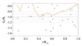
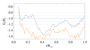
Figure 1: Radial profiles of the ${\cal G}_{r}/{\cal H}_{r}$ ratio for one simulated cluster (D8) of the sample. Left: mean (black crosses) and median (orange, solid line) profiles calculated from the particle-by-particle values of ${\cal G}_{r}/{\cal H}_{r}$; right: mean (black, dashed line) and median (orange, solid line) ${\cal G}_{r}/{\cal H}_{r}$ profiles calculated from the radial profiles of the two separate components ${\cal G}_{r}$ and ${\cal H}_{r}$.

It is important to notice that (b) and (d) are derived from the left- and right-hand-side terms of Eq. (1) but do not share the same assumptions, as purely thermal pressure is assumed only when $M_{\rm HE}$ is calculated.

4 Results

4.1 Application to simulated galaxy clusters

By applying the method described in the previous section to simulated galaxy clusters, we can gain a deeper understanding of the intrinsic state of the ICM, in the presence of several astrophysical phenomena, such as star formation, feedback processes, and accretion of substructures. Moreover, we can explore the validity of the HE assumption and its influence on the median behaviour in different population of clusters.

For the purpose of showing how complex is the level of HE deviation at different radii, we start by considering one single object shown in Figure 1.

We notice the evident difference between the methods $(i)$ and $(ii)$ described in Section 3. In particular, both the mean (black, dashed curve) and median profiles (orange, solid curve) are smoother when we measure the ratio of the two profiles (see right panel in Figure 1).

The different picture drawn from the particle-based approach (left panel in Figure 1) can be ascribed to the inhomogeneous distribution of the gas accelerations and to the large spread of the hydrodynamical acceleration values, which is considerably broader than the gravitational one. Furthermore, the kernels used to smooth the hydrodynamical and gravitational forces are different. Therefore, the accelerations are evaluated at two unequal scales. Furthermore, numerical terms (e.g. artificial viscosity and diffusion) intervene in the SPH implementation of the Euler equation, so that Eq. (1) is not satisfied in its theoretical formulation on a particle base. In the following we use the second approach where we compute the two ${\cal G}_{r}$ and ${\cal H}_{r}$ components separately and subsequently we calculate the ratio ${\cal G}_{r}/{\cal H}_{r}$ from their profiles.

The cluster shown in Figure 1 represents a rather extreme case, with deviations up to $\sim 50$ per cent or more, already outside the inner region ($>0.1\,R_{\rm vir}$), indicating a non-negligible violation of the HE assumption and possible biases in the HE-derived mass estimate.

In general, among the 29 clusters of the sample, the individual profiles show significant variations and a close inspection to the distribution of each cluster substructures, merging and thermal history would be necessary to understand the detailed features of the ${\cal G}_{r}/{\cal H}_{r}$ profiles.

4.2 On the relation to the hydrostatic mass bias

D5

D24

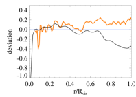
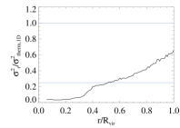
D8

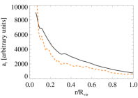
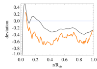
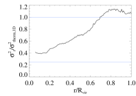
Figure 2: Three different clusters (D5, D24 and D8) in the sample, chose to represent two extreme cases and an intermediate one w.r.t. the comparison between the deviation from HE, traced by $\delta_{\rm HE}={\cal G}_{r}/{\cal H}_{r}+1$, and mass bias $b_{M}$. From left to right we show the radial profiles of: the gravitational (${\cal G}_{r}$, changed in sign; black solid line) and hydrodynamical (${\cal H}_{r}$; orange dashed line) accelerations (radial components); mass bias ($b_{M}$; black line) and deviation from HE ($\delta_{\rm HE}$; orange thick line); amount of non-thermal motions along the radial direction, with respect to thermal ones.

For each cluster in the sample we calculate the hydrostatic mass as in Eq. (4). For the purpose of our theoretical investigation, we do not apply any substructure removal from the ICM. In principle, the hydrostatic mass bias, $b_{M}$ (definition (e), in section 3), does quantify the deviation from HE as long as the additional hypotheses on which the hydrostatic mass relies are valid. Therefore, it is interesting to compare the radial profiles of ${\cal G}_{r}/{\cal H}_{r}$ and mass bias.

In order to explore the origin of the differences between mass bias and deviation from HE, it is also useful to investigate possible connections to the level of non-thermal motions of the gas, which are typically not accounted for in the usual hydrostatic mass estimate.

In Figure 2 we present, for three clusters of the sample, the separate profiles of the two accelerations (left panels), the direct comparison of mass bias and deviation from HE (central panels), and the ratio $\sigma^{2}_{r}/\sigma^{2}_{\rm therm,1D}$ (right panels), where $\sigma^{2}_{r}$ is the velocity dispersion of the gas in the radial direction and $\sigma^{2}_{\rm therm,1D}$ is the expected one-dimensional thermal velocity dispersion, The thermal velocity dispersion, instead, is calculated as

$$\sigma^{2}_{\rm therm}=\frac{3k_{B}T_{\rm mw}}{\mu m_{p}},$$

where $T_{\rm mw}$ is the mass weighted temperature in the shell and for a single dimension $\sigma^{2}_{\rm therm,1D}=\sigma^{2}_{\rm therm}/3$. in the same radial bin. The last quantity represents the excess of the velocity dispersion produced by bulk and random motions over that produced by thermal motions.

The top- and bottom-row panels represent the opposite cases where the profiles of $b_{M}$ and $\delta_{\rm HE}$ either trace each other in a very good way (as for D5) or show a significant off-set (D8). In the first case, the mass bias more directly reflects the level of deviation from HE, suggesting that the additional assumption of purely thermal pressure support — included in $M_{\rm HE}$, but not involved in $\delta_{\rm HE}$ — does not play a significant role. This is in fact supported by the low amount of non-thermal motions, with respect to thermal ones, shown in the right panel. Viceversa for D8, we notice a systematic difference between $b_{M}$ and $\delta_{\rm HE}$, with the latter much more significant than the mass bias, throughout the whole radial range. The origin of the significant deviation from HE on the radial direction is due to the systematic unbalance between the two forces, as visible from the separate ${\cal G}_{r}$ and ${\cal H}_{r}$ profiles in the left panel. The mismatch between $b_{M}$ and $\delta_{\rm HE}$ is strongly connected with the behavior of the $\sigma^{2}_{r}/\sigma^{2}_{\rm therm,1D}$ ratio, which significantly increases from 0.4 in the center out to more than one towards the virial radius, indicating that outside $\sim 0.7R_{\rm vir}$ macroscopic non-thermal motions actually start to be dominant.

The halo presented in the middle row of Figure 2 (D24) represents instead an intermediate case where, despite the low-level deviation from ${\cal G}_{r}/{\cal H}_{r}=-1$ ($\delta_{\rm HE}$, mostly around $10$ per cent out to the virial radius), the mass bias profile does show a different trend, especially towards the outer regions. The modulus of ${\cal G}_{r}/{\cal H}_{r}$ decreases with increasing radius, indicating that ${\cal H}_{r}$ dominates over ${\cal G}_{r}$, whereas the mass bias suggests the opposite unbalance between the hydrodynamical and the gravitational forces: $b_{M}<0$, indeed, indicates that the thermal pressure support under-estimates the gravitating mass.

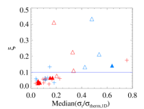
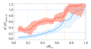
Figure 3: Left: relation between the median difference between the profiles of mass bias and deviation from HE (quantified by $\xi$; see Eq. (6)), and the median value of the $\sigma^{2}_{r}/\sigma^{2}_{\rm therm,1D}$ ratio, within $R_{\rm 500}$, for the 29 clusters in the sample. The horizontal line marks the threshold used to identify the subsample of clusters with large(small) differences between the $b_{M}$ and $\delta_{\rm HE}$ profiles, i.e. with $\xi>0.1$($<0.1$). The symobls and colors refer to the two classifications used to subdivide the sample, as specified in the following Section 4.4. Right: median radial profile of the $\sigma^{2}_{r}/\sigma^{2}_{\rm therm,1D}$ ratio, distinguishing between two classes of clusters, i.e. those with $\xi<0.1$ (blue solid line) and $\xi>0.1$ (red dot-dashed line), within $R_{\rm 500}$. Shaded areas mark the median absolute deviation in each radial bin. From left to right, vertical lines mark median values of $R_{\rm 2500}$, $R_{\rm 500}$ and $R_{\rm 200}$, respectively.

The trend shown by the three examples in Figure 2 is in fact present in the entire sample, with large deviations from HE generally associated to substantial non-thermal motions of the gas. Furthermore, we notice that the profiles of ${\cal G}_{r}$ and ${\cal H}_{r}$ (left panels) indicate that the gravitational component is typically smoother than the hydrodynamical one and that haloes with large deviations from HE also show a large offset of ${\cal H}_{r}$ with respect to ${\cal G}_{r}$, with the latter generally dominating in modulus. In general, the origin of deviations from HE and its relation to the mass bias can significantly vary from cluster to cluster, requiring a dedicated investigation of the particular cluster properties. Nonetheless, from the analysis of all the 29 clusters, we can conclude that large differences between $b_{M}$ and $\delta_{\rm HE}$ typically correspond to $\sigma^{2}_{r}\gtrsim 0.3\,\sigma^{2}_{\rm therm,1D}$, as observed for example in the extreme case of cluster D8, where $\sigma^{2}_{r}/\sigma^{2}_{\rm therm,1D}$ is larger than 40 per cent from the center out to the virial radius.

From a more quantitative perspective, we provide a measure of the typical difference between the two radial profiles of $b_{M}$ and $\delta_{\rm HE}$ as the median value of the absolute difference among the two, i.e.

$$\xi={\rm Median}(|b_{M}-\delta_{\rm HE}|),$$ (6)

considering the radial range up to $R_{\rm 500}$. The motivation to consider the region enclosed by $R_{\rm 500}$ is that this is an optimal region targeted also by observational analyses, while outer portions of the cluster regions are generally more difficult to characterize. Furthermore, the amount of non-thermal motions in the radial direction generally increases towards the outskirts, where merging and accretion processes play a more significant role, for all the clusters. Also, the use of the median deviation allows us to estimate the typical difference between the two profiles, without being biased by large differences restricted to few radial bins. As visible from the left panel in Figure 3, it is possible to identify a subsample of clusters for which the median difference between the $b_{M}$ and $\delta_{\rm HE}$ radial profiles, $\xi$, and the median value of $\sigma^{2}_{r}/\sigma^{2}_{\rm therm,1D}$, are both very low within $R_{\rm 500}$. From this figure, we use the threshold $\xi=0.1$ to separate these systems from those with larger values of both the indicators. The median radial profile of $\sigma^{2}_{r}/\sigma^{2}_{\rm therm,1D}$ for these two subsamples of clusters is shown in the r.h.s. panel of Figure 3, where the red, dot-dashed curve represents the subsample with typically different $b_{M}$ and $\delta_{\rm HE}$ profiles, while the blue, solid line indicates those with more similar ones ($\xi<0.1$). The comparison of the two profiles confirms that larger differences between the $b_{M}$ and $\delta_{\rm HE}$ profiles (red curve) correspond to larger ($>30\%$) amount of non-thermal over thermal motions (in the radial direction), despite the larger dispersion in the subsample that only comprises 9 systems out of 29. We additionally note that the systematic offset visible out to $R_{\rm 500}$, that is in the region where the classification criteria are defined (Figure 3, left panel), is still present almost out to $R_{\rm 200}$ ($\sim 0.7R_{\rm vir}$). Both subsamples, instead, behave more similarly in the outermost region, where in fact the $\sigma^{2}_{r}/\sigma^{2}_{\rm therm,1D}$ ratio increases for both classes.

As displayed by Figure 9 below, a similar behaviour is recognised when the subsample is instead divided in regular and disturbed systems, with the second class typically showing a higher profile of the non-thermal to thermal motion ratio.

4.3 Average deviation from HE

Overall, our results confirm that not only the hydrostatic mass bias, but also the level of deviation from the static assumption, $\delta_{\rm HE}$, is in fact very different from cluster to cluster and at different radii within the single object. This is consistent with the findings obtained in similar works based on AMR simulations (e.g. Shi et al., 2015; Nelson et al., 2014; Lau et al., 2013).

A possible way to investigate the problem is to consider samples of clusters and stack the individual profiles to infer an average behaviour. In this way, the effects due to asphericity of the individual clusters are alleviated and the importance of the assumption of spherical symmetry is less significant.

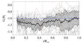
Figure 4: Median radial profile (black solid curve) of the ratio between the radial components of gravitational and hydrodynamical acceleration, for the main haloes in the 29 re-simulated regions. The light-grey lines in the background represent the individual ${\cal G}_{r}/{\cal H}_{r}$ profiles of all the 29 haloes. From left to right, vertical lines mark median values of $R_{\rm 2500}$, $R_{\rm 500}$ and $R_{\rm 200}$, respectively. We indicate with the shaded area the median absolute deviation from the the median profile.

The stack analysis is shown in Figure 4, where we display the individual profiles (grey curves) and the median one (black). The shaded area indicates the dispersion of the distribution in each radial bin around the median value, and is computed as the median absolute deviation. As pointed out, the background individual profiles show very different features and the overall dispersion increases with the radius. In the outskirts, where the gas acceleration field is more sensitive to substructure infalling onto the main halo, the spread is larger. Nevertheless, the median profile indicates that the typical deviation of ${\cal G}_{r}/{\cal H}_{r}$ from $-1$ is $\sim 10$ per cent, reaching $\sim 20$ per cent at most.

Similarly, we can construct the median profile of the mass bias for the 29 haloes in the sample, as shown in Figure 5.

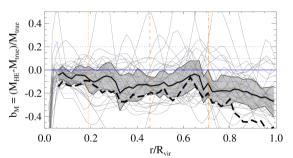
Figure 5: Median radial profile of the mass bias $b_{M}$, with $M_{\rm HE}$ calculated for both $T=T_{\rm mw}$ (black solid line) and $T=T_{\rm sl}$ (black dashed line). Only for the first case ($T=T_{\rm mw}$), we also report the individual mass-bias profiles of the 29 clusters (light-grey curves) and the median absolute deviation from the median profile (shaded area). From left to right, vertical lines mark median values of $R_{\rm 2500}$, $R_{\rm 500}$ and $R_{\rm 200}$, respectively.

Without distinguishing the dynamical state of clusters, from the comparison between Figures 4 and 5 we see that the two median profiles of acceleration term and hydrostatic mass bias are quite similar out to $\sim 0.7\,R_{\rm vir}$ (roughly $\sim R_{\rm 200}$). This suggests that the negative mass bias does trace — on average — the violation of HE, i.e. the equilibrium is not static and the (total) acceleration term is non zero.

The computation of the hydrostatic mass as in Eq. (4) from X-ray data can include an additional bias due to the under-estimate of the X-ray temperature with respect to the dynamical temperature. A good approximation for the temperature measured by Chandra and XMM-Newton telescopes is provided by the so-called spectroscopic-like temperature $T_{\rm sl}$ Mazzotta et al. (2004), which is commonly used in numerical simulations and it is defined as

$$T_{\rm sl}=\frac{\Sigma_{i}w_{i}T_{i}}{\Sigma_{i}w_{i}}\qquad\mbox{with}\quad w_{i}=m_{i}\rho_{i}T_{i}^{-3/4}\,.$$ (7)

In Eq. (7) $m_{i},\rho_{i},T_{i}$ indicate the mass, density and temperature of the single gas element in the simulation. It has been shown in previous works (e.g. Biffi et al., 2014) that due to the presence of inhomogeneities in the X-ray emitting gas there is a systematic difference between the spectroscopic-like estimate and the mass-weighted temperature ($T_{\rm mw}$) that would introduce an additional bias in $M_{\rm HE}$ (e.g. Rasia et al., 2014). The origin of such bias is however independent of the assumptions of HE or purely thermal pressure support, and only depends of the degree of thermal complexity of the ICM.

When the spectroscopic-like temperature $T_{\rm sl}$ is adopted, instead of $T_{\rm mw}$, we observe the additional bias (black dashed curve in Figure 5) due to the different temperature estimation. In this case the average bias ranges from $\sim 15$ per cent to $\sim 25$ per cent within $R_{\rm 200}$, while it is more significant in the cluster outer regions, increasing up to 50 per cent.

Focusing on the outskirts, the trend of the average mass bias profile is different from the ${\cal G}_{r}/{\cal H}_{r}$ one. Given the likely presence of infalling substructures, the hydrostatic estimate is on average significantly lower than the true mass, although the deviation from HE (quantified via ${\cal G}_{r}/{\cal H}_{r}$) is typically closer to zero. This suggests that at such large radii the origin of the mass bias is mostly related to the additional assumption of the purely thermal nature of the ICM pressure, involved in the computation of $M_{HE}$, rather than to a pure violation of the static state $d{\bf v}/dt=0$. Nevertheless, we remind that ${\cal G}_{r}/{\cal H}_{r}\sim-1$ only asserts the equilibrium in the radial direction, and differences in the anisotropy of the two acceleration components can also play a role, especially in the outskirts.

4.4 Distinguishing among cluster populations

We proceed to evaluate the median mass bias and the $\delta_{\rm HE}$ profiles for subsamples defined on the basis of either their thermal or dynamical processes. In particular, we consider here two classifications: (a) one linked to the cool-coreness of the object and (b) the other to its global dynamical state. These two classifications are typical ways of distinguishing regular/disturbed clusters in observational (method a) and numerical (method b) studies.

Cool-coreness.

The classification (a) is based on the core thermal properties of the clusters, and specifically on the central entropy value. In more detail, we define the cluster as cool core (CC) if

$${\rm CC}:\left\{\begin{aligned} K_{0}&<60\rm{\,keV}/{\rm cm}^{2}\\ \sigma&<0.55\end{aligned}\right.$$ (8)

and non cool core (NCC) otherwise (see Rasia et al., 2015, for more details on this classification). In Eq. (8) $K_{0}$ is the central entropy derived from the fit of the cluster entropy profile, and $\sigma$ is the pseudo-entropy, defined as $\sigma=(T_{\rm IN}/T_{\rm OUT})*({\rm EM}_{\rm IN}/{\rm EM}_{\rm OUT})^{-1/3}$, with the temperature (T) and Emission Measure (EM) computed within the “IN” and “OUT” regions, corresponding to $R<0.05\,R_{\rm 180}$ and $0.05\,R_{\rm 180}<R<0.2\,R_{\rm 180}$, respectively (see, e.g., Rossetti et al., 2011).

With this method we classify 11 clusters out of 29 as CC, and the remaining 18 haloes as NCC.

Dynamical state.

The method (b), instead, combines two criteria commonly used in numerical simulations to classify a cluster as dynamically regular or disturbed: the center shift ($\delta r$), defined as the spatial separation between the position of the minimum of the potential and the center of mass, and the fraction of mass associated to substructures ($f_{\rm sub}$). In our work, we define regular clusters those for which

$$\left\{\begin{aligned} \delta r=~{}&||{\bf x}_{\rm min}-{\bf x}_{\rm cm}||/R_{\rm 200}&<&~{}0.07&\\ f_{\rm sub}=~{}&\frac{M_{\rm tot,sub}}{M_{\rm tot}}&<&~{}0.1&\end{aligned}\right.\,,$$ (9)

where ${\bf x}_{\rm min}$ and ${\bf x}_{\rm cm}$ are, respectively, the position of the minimum of the potential and the center of mass, $M_{\rm tot}$ is the total mass and $M_{\rm tot,sub}$ is the total mass in substructures. For values of $\delta r$ and $f_{\rm sub}$ above those thresholds the clusters are classified as disturbed. Similar conditions are adopted in Neto et al. (2007) and Meneghetti et al. (2014). Those systems for which the two criteria in (9) are not simultaneously satisfied are classified as intermediate systems. This second classification defines the state of the cluster on more global scales, with the quantities above calculated for each cluster within $R_{\rm 200}$.

With this method we split the sample of 29 clusters into 6 regular and 8 disturbed systems, and 15 intermediate cases.

4.4.1 The ratio ${\cal G}_{r}/{\cal H}_{r}$

In the two panels of Figure 6 we show that the median profile of ${\cal G}_{r}/{\cal H}_{r}$ depends on the classification assumed.

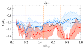
Figure 6: Median radial profile of ${\cal G}_{r}/{\cal H}_{r}$, as in Figure 4, distinguishing among different cluster populations. Shaded areas represent the median absolute deviation in each radial bin (w.r.t. the median value). Upper panel: CC/NCC (blue solid/red dot-dashed line); lower panel: regular/disturbed (blue solid/red dot-dashed line) clusters; intermediate systems are marked by the thin black line and, for simplicity, no dispersion is marked. From left to right, vertical lines mark median values of $R_{\rm 2500}$, $R_{\rm 500}$ and $R_{\rm 200}$, respectively.

When the sample is divided into CC and NCC clusters, as in the upper panel of Figure 6, there is no significant difference in the ${\cal G}_{r}/{\cal H}_{r}$ profile of the two populations, especially considering the dispersion around the median values. Overall, both behaviours are very similar to the median profile constructed from the whole sample (Figure 4).

A different picture emerges when the selection is made on the global dynamical properties. In this case (lower panel of Figure 6) the two populations show a clearer sistematic offset, especially outside $R_{\rm 2500}$, with the largest departure in the region outside $R_{\rm 200}$ ($\sim 0.7$–$0.9\,R_{\rm vir}$). We find that the median profile of regular clusters is systematically higher and closer to the HE value of $-1$. On the contrary disturbed clusters show a larger ($>20$ per cent) deviation from HE throughout the radial range.

We notice that this difference is not due to the presence of an intemediate class in the dynamical classification, which has no analogue in the CC-NCC one. In fact, by restricting the NCC subsample to the most extreme cases and thus introducing an intermediate class of objects, a similar separation to that observed between regular and disturbed clusters is still not found.

It is important to note that our sample of disturbed clusters are likely to be more strongly affected by merging events and accretion of infalling substructures, as confirmed also by their clumpiness profiles, presented by Planelles et al. (in prep.). This should also reflect into a more significant difference in the (an)isotropy of the gravitational and hydrodynamical acceleration fields, likely to be enhanced at larger distances from the cluster center where the mass assembly is still ongoing.

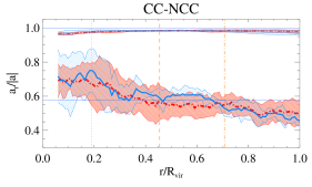
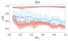
Figure 7: Median radial profile of the ratio between the radial component of the acceleration and the modulus of the total acceleration vector. This ratio quantifies the anisotropy of the — gravitational and hydrodynamical (thin and thick lines, respectively) — acceleration field: $a_{r}/|{\bf a}|=1\rightarrow$ purely radial, $a_{r}/|{\bf a}|=1/\sqrt{3}\rightarrow$ isotropic (both marked by blue solid lines), and $a_{r}/|{\bf a}|=0\rightarrow$ purely tangential. Shaded areas represent the median absolute deviation from the median value in each radial bin. Upper panel: CC/NCC (blue solid/red dot-dashed line); lower panel: regular/disturbed (blue solid/red dot-dashed line) clusters; intermediate systems are marked by the thin black line and, for simplicity, no dispersion is marked. From left to right, vertical lines mark median values of $R_{\rm 2500}$, $R_{\rm 500}$ and $R_{\rm 200}$, respectively.

In fact, we see from Figure 7 (bottom panel) that the gravitational acceleration is generally almost radial from the center out to the outskirts (typically ${\cal G}_{r}$$/|{\bf a}_{g}|\sim 0.9$), while the hydrodynamical acceleration shows a radial component which decreases with radius (from $\sim 0.7$ to $\sim 0.5$, going from the center to $R_{\rm 200}$) and is almost isotropic in the intermediate region comprised between $R_{\rm 500}$ and $R_{\rm 200}$. This is more evident for disturbed clusters, for which the profile of ${\cal H}_{r}$$/|{\bf a}_{h}|$ is systematically lower, namely less radial, than for regular systems. This off-set is mirrored by the one in the ${\cal G}_{r}/{\cal H}_{r}$ profiles.

Instead, the same is not observed when the dinstiction between CC and NCC systems is adopted, as shown in the upper panel of Figure 7. In this case, the profiles of the two populations behave in a very similar way, for both the acceleration components.

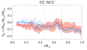
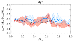
Figure 8: Median radial profile of the mass bias, as in Figure 5, distinguishing among different cluster populations. Upper panel: CC/NCC (blue solid/red dot-dashed line); lower panel: regular/disturbed (blue solid/red dot-dashed line) clusters; intermediate systems are marked by the thin black line and, for simplicity, no dispersion is marked. The hydrostatic mass, $M_{\rm HE}$, is calculated using $T_{\rm mw}$. Shaded areas represent the median absolute deviation from the median value, in each radial bin. From left to right, vertical lines mark median values of $R_{\rm 2500}$, $R_{\rm 500}$ and $R_{\rm 200}$, respectively.

4.4.2 Hydrostatic mass bias

Using the same selection criteria to investigate the mass bias we obtain the results presented in Figure 8 (upper and lower panel, respectively). Here we only show the results for $M_{\rm HE}$ computed using the mass-weighted temperature, altough we verified that using the spectroscopic-like estimate we obtain very similar profiles, with the only difference of an overall more significant bias (as seen from Figure 5) and a larger scatter, especially outside $R_{\rm 200}$.

We note that the hydrostatic mass bias behaves differently from the acceleration term with respect to the classification adopted: no sistematic distinction between regular and disturbed clusters is evident, except for the outermost region ($>0.7R_{\rm vir}$). Instead, a separation, albeit relatively mild, is found between CC and NCC out to $\sim R_{\rm 2500}$, where there is an offset between their median profiles and the shaded areas marking the dispersion around the median values barely touch each other. In that inner region of the radial profile, the CC population presents almost zero mass bias while the NCC subsample is characterised by a mass bias of roughly $10$–$15$ per cent. This is mainly due to the different thermo-dynamical properties of the two classes in the innermost region, where CC clusters are typically characterized by a higher thermal pressure support with respect to NCC systems (see Planelles et al., in prep.), despite the similar shape of their potential well. This then reflects in a better match between the hydrostatic mass and total gravitating mass.

Interestingly, the comparison between the lower panels of Figures 8 and 6 indicates that the hydrostatic mass bias of disturbed systems is on average $\lesssim 25$ per cent (with peaks around $25$–$30$ per cent) despite the larger deviation from $-1$ of ${\cal G}_{r}/{\cal H}_{r}$ (mostly $\delta_{\rm HE}>20$ per cent, up to $50$ per cent). The origin of a deviation from zero acceleration (on the radial direction) that is larger than the violation of the balance between gravitational and thermal pressure forces, must be related to gas non-thermalized motions, that are not accounted for in our computation of $\nabla P$ (where $P=P_{\rm th}\propto\rho\,T$).

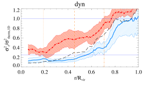
Figure 9: Median radial profile of $\sigma^{2}_{r}/\sigma^{2}_{\rm therm,1D}$, distinguishing among different cluster populations. Upper panel: CC/NCC (blue solid/red dot-dashed line); lower panel: regular/disturbed (blue solid/red dot-dashed line) clusters; intermediate systems are marked by the thin black line and, for simplicity, no dispersion is marked. Shaded areas represent the median absolute deviation from the median value, in each radial bin. From left to right, vertical lines mark median values of $R_{\rm 2500}$, $R_{\rm 500}$ and $R_{\rm 200}$, respectively.

From Figures 6 and 7 (and Figure 9 below) we conclude that the radial properties of the ICM acceleration field, and thus the level of HE, are not very sensitive to the cool-coreness of the system, but rather depend on its global dynamical state, whereas the mass bias is more closely related to the cool-coreness, and so to thermal properties, especially in the central regions (see Figure 8).

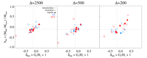
Figure 10: Relation between mass bias ($b_{M}$) and deviation from HE ($\delta_{\rm HE}$), calculated at $R_{\rm 2500}$ (left), $R_{\rm 500}$ (middle) and $R_{\rm 200}$ (right). In each panel median values of the distributions are indicated by the dotted lines.

	$\Delta=2500$	$\Delta=500$	$\Delta=200$
$b_{M}$
all	$-0.091\pm 0.016$	$-0.123\pm 0.015$	$-0.120\pm 0.024$
CC	$-0.001\pm 0.027$	$-0.132\pm 0.017$	$-0.140\pm 0.020$
NCC	$-0.123\pm 0.011$	$-0.119\pm 0.021$	$-0.102\pm 0.036$
regular	$-0.118\pm 0.015$	$-0.095\pm 0.031$	$-0.065\pm 0.080$
disturbed	$-0.080\pm 0.035$	$-0.148\pm 0.060$	$-0.162\pm 0.024$
$\delta_{\rm HE}$
all	$-0.148\pm 0.022$	$-0.148\pm 0.016$	$-0.173\pm 0.039$
CC	$-0.017\pm 0.046$	$-0.168\pm 0.049$	$-0.175\pm 0.055$
NCC	$-0.157\pm 0.019$	$-0.132\pm 0.024$	$-0.101\pm 0.057$
regular	$-0.178\pm 0.024$	$-0.096\pm 0.027$	$-0.010\pm 0.081$
disturbed	$-0.247\pm 0.047$	$-0.287\pm 0.080$	$-0.281\pm 0.044$

Table 1: Median values and errors of the mass bias (top, $b_{M}$) and deviation from HE (bottom, $\delta_{\rm HE}$) reported in Fig. 10, calulated at $R_{2500}$, $R_{500}$ and $R_{200}$ and for the various subsamples considered.

Differences between the ${\cal G}_{r}/{\cal H}_{r}$ and mass bias radial profiles can also be related to the presence of non-thermal, bulk and random, motions in the gas, as discussed in Section 4.2. Here, we present median stacked profiles of $\sigma^{2}_{r}/\sigma^{2}_{\rm therm,1D}$ for the subsamples defined on the basis of the cluster cool-coreness or dynamical classification, in analogy to Figures 6 and 8. From Figure 9, we infer that CC and NCC (upper panel) behave in a very similar way, with a similar amount of non-thermal motions increasing towards larger distances from the center. On the contrary, disturbed systems clearly differentiate from dynamically regular ones (lower panel) for the presence of a more substantial amount of radial non-thermal motions with respect to thermal ones already in the innermost region and out to the virial radius (systematically higher values of $\sigma^{2}_{r}/\sigma^{2}_{\rm therm,1D}$). So the conclusion is that mass bias and HE-violations are two different things, the first more related to cool-coreness, the second more related to the dynamical state of the cluster.

In addition to their radial dependence, it is useful to evaluate the relation between mass bias and deviation from HE at interesting distances from the cluster center, such as $R_{\rm 2500}$, $R_{\rm 500}$ and $R_{\rm 200}$ (see Fig. 10). Despite a larger scatter in the outskirts, the two quantities closely trace each other, as indicated by the Pearson correlation coefficient for the three relations: 0.73, 0.72, 0.69, for $R_{\rm 2500}$, $R_{\rm 500}$ and $R_{\rm 200}$, respectively. The significance of this result is confirmed by corresponding p-values of the correlation coefficients of $8.1\cdot 10^{-6}$, $1.1\cdot 10^{-5}$ and $3.3\cdot 10^{-5}$. In particular, this result is stronger for the subsample of regular systems, for which the correlation coefficients range from 0.88 at $R_{\rm 2500}$ to 0.86 at $R_{\rm 200}$ (with p-values of order of 0.02–0.03). Then, mass bias and violation of HE are correlated with each other despite reflecting different aspects of clusters. The outliers of this correlation tend to be disturbed clusters and typically reside in the upper envelope of the relation (higher $b_{M}$ and lower $\delta_{\rm HE}$ than expected from the linear correlation).

In Table 1 we report the median values, with 1-$\sigma$ errors, of the $b_{M}$ and $\delta_{\rm HE}$ distributions shown in Fig. 10. We note that these results correspond to single radial bins (at $R_{\rm 2500}$, $R_{\rm 500}$ and $R_{\rm 200}$, respectively) in the profiles discussed in the previous sections.

Figure 11: Left: radial profile of the temperature bias $b_{T}=(T_{\rm sl}-T_{\rm mw})/T_{\rm mw}$, for the 29 main haloes of this work (top panel). In the bottom panel the median profiles for CC and NCC are shown. Colors refer to CC (blue) and NCC (red) clusters, as in the legend. Right: temperature bias as a function of $T_{\rm mw}$, for the average temperatures within $R_{\rm 500}$, for the 29 haloes; color code marks the CC/NCC (blue/red) classification while symbols distinguish among regular, disturbed and intermediate systems.

Figure 12: Dependence of mass bias ($b_{M}$; upper panels) and deviation from HE ($\delta_{\rm HE}$; lower panels) on the temperature bias ($b_{T}$), calculated at $R_{\rm 2500}$ (left), $R_{\rm 500}$ (middle) and $R_{\rm 200}$ (right). In each panel median values of the distributions are indicated by the dotted lines.

4.5 Correlation with temperature bias

For the purpose of our investigation, it is finally important to explore the thermal structure of the ICM and the presence of temperature inhomogeneities, which might affect both the level of hydrostatic equilibrium and the bias on the hydrostatic mass therefrom derived.

Numerically, this can be evaluated by comparing the mass-weighted and spectroscopic-like estimates of temperature, $T_{\rm mw}$ and $T_{\rm sl}$, where the former is a more dynamical measurement while the latter is more sensitive to the multi-phase nature of the gas.

One common way of evaluating this is to calculate the so-called temperature bias, defined as

$$b_{T}=(T_{\rm sl}-T_{\rm mw})/T_{\rm mw}\,.$$ (10)

In Figure 12 we report the radial profile of the temperature bias for the 29 haloes (left panel, top), for which we also show the median profiles for the CC and NCC populations, separately (left panel, bottom). On average, $b_{T}$ is always negative out to the virial radius, indicating that, locally, the spectroscopic-like temperature typically under-estimates the dynamical measurement ($T_{\rm mw}$), at all distances from the cluster center. Nevertheless, the average bias is found to be quite small, indicating a relatively homogeneous temperature structure for both categories, out to $\sim R_{\rm 500}$ (i.e. $\sim 0.4R_{\rm vir}$), with $b_{T}\lesssim 10$ per cent. This can be explained by the improved gas mixing that characterises these new simulation runs, which allows the gas stripped from the substructures to efficiently mix and better thermalize with the surrounding ambient ICM. In the innermost cluster region the difference between CC and NCC temperature profiles, decreasing in the first case and flattening or even rising in the other, is not caught by the temperature bias profile. The reason for this is that the region sampled by each central radial bin is not extended enough to capture the central temperature gradient typical of CC. In the outer part of the profile, enclosed between $R_{\rm 500}$ and $R_{\rm 200}$, the bias remains relatively low for CC systems, whereas the mismatch between $T_{\rm sl}$ and $T_{\rm mw}$ increases for NCC. Towards the virial radius, the bias significantly increases for both classes.

In the right-hand-side panel of Figure 12 we report the direct comparison of the global estimates of $T_{\rm mw}$ and $T_{\rm sl}$, for the region enclosed by $R_{\rm 500}$, by showing the temperature bias as a function, e.g., of $T_{\rm mw}$. Considering the large variety of dynamical states among the clusters in the sample, we observe on average a very good agreement between the two values, with $T_{\rm sl}$ typically underestimating $T_{\rm mw}$ by only few percents (within $R_{\rm 500}$, the median value of the bias is $\sim 5$). From this relation we also note that there is no evidence for a dependence of the temperature bias on the global dynamical temperature of the systems. In fact, given the well-defined relation between temperature and mass for the clusters analysed (see Truong et al., in preparation), we also verified that there is no clear dependence of the temperature bias on the total cluster mass.

Hydrostatic equilibrium is however a local condition and ultimately depends on the local thermodynamical properties of the ICM. Thus, it is interesting to evaluate the relation between deviation from HE, mass bias and temperature bias, as in Figure 12, via the dependence of $b_{M}$ and $\delta_{\rm HE}$ (in the upper and lower panels, respectively) on the $b_{T}$, at interesting distances from the cluster center, i.e. $R_{\rm 2500}$, $R_{\rm 500}$ and $R_{\rm 200}$.

Marking the clusters with different symbols and colors, depending on their cool-coreness or dynamical classification, we mainly note a difference between regular and disturbed systems (filled and empty symbols in the Figure), especially in terms of scatter, which is significantly larger for the disturbed ones. This is particularly evident for the values corresponding to $R_{\rm 500}$ and $R_{\rm 200}$, where there is a more clear separation between the two dynamical classes, especially in terms of temperature bias.

Overall, we conclude from Figure 12 that the local level of HE and mass bias are not significantly affected by the local inhomogeneities in the ICM temperature structure. This is quantified by very low values of the Pearson correlation coefficients of the $b_{M}$-$b_{T}$ and $\delta_{\rm HE}$-$b_{T}$ relations, which only reach a maximum of $\sim 0.3$ for $R_{\rm 500}$ and is very poorly constrained (p-values $>0.1$). Only the CC subsample shows evidences for a significant correlation between $\delta_{\rm HE}$ and temperature bias, especially in the outskirts — with a Pearson correlation coefficient(p-value) of $\sim 0.68$($0.02$) at $R_{\rm 500}$ and $\sim 0.66$($0.03$) at $R_{\rm 200}$.

5 Discussion and conclusion

The violation of hydrostatic equilibrium in galaxy clusters has been widely studied from the numerical point of view, in order to trace its origin and the connection to the bias in the mass reconstruction based on the HE hypothesis.

Here, we explored the violation of HE in the ICM by studying the balance between gravitational and hydrodynamical acceleration, on the radial direction. This allowed us to investigate the level of deviation from HE per se, i.e. separately from the mass bias, which additionally implies the assumption of purely thermal pressure support (with $P_{\rm th}\propto\rho\,T$).

In the following we summarize our main findings.

• Corrections for HE-violation based on the acceleration term for individual clusters are not really achievable. The differences from case to case, and depending on the distance from the cluster center, make the prediction of a single correction term very challenging, even by means of numerical simulations. This is noticeable from the significant scatter in the radial profiles of ${\cal G}_{r}/{\cal H}_{r}$.

• The classification of relaxed and un-relaxed clusters can be misleading, especially when simulations and observations are compared: depending on which cluster properties are used to define the level of regularity, the differences among the populations range from substantial to negligible. Caution is necessary when numerical results, e.g. scaling relations, are compared to observed ones, and vice versa.

• The acceleration term, quantified via the ${\cal G}_{r}/{\cal H}_{r}$ ratio, shows a systematic difference between the median radial profile of dynamically regular clusters and that of disturbed ones, with the latter showing a larger deviation from HE ($\delta_{\rm HE}>20$ per cent), i.e. from $d{\bf v}/dt=0$ (on the radial direction). This is especially significant in the outskirts ($\delta_{\rm HE}\sim 50$ per cent).

  Instead, we find no clear dependence of the ${\cal G}_{r}/{\cal H}_{r}$ profile on the system cool-coreness, from comparing CC and NCC median profiles.

• On the contrary, when the hydrostatic mass bias is concerned, CC and NCC clusters behave differently, especially in the inner region ($\lesssim R_{\rm 2500}$), whereas no siginificant distinction is observed between the mass bias of regular and disturbed clusters, given the large dispersion.

• Typically, we find that the clusters for which the radial profile of mass bias and deviation from HE ($\delta_{\rm HE}$) poorly trace each other present a significant amount of non-thermal (bulk and random) gas motions with respect to thermal ones, in the radial direction, quantified by $\sigma^{2}_{r}/\sigma^{2}_{\rm therm,1D}>0.3$ already in the innermost regions.

• We find also a clear correlation between values of the hydrostatic mass bias and the deviation from HE computed at $R_{\rm 2500}$, $R_{\rm 500}$ and $R_{\rm 200}$, with the main outliers in this picture represented by dynamically disturbed systems. From this we conclude that the local deviation from HE is of order 15–20 per cent (increasing towards the outskirts), and it is generally well traced by the local mass bias (of order 10–15 per cent).

• The temperature structure of the clusters in the sample appears to be relatively regular, with a temperature bias lower than what previously found in SPH simulations. In fact we find that $T_{\rm sl}$ typically underestimates $T_{\rm mw}$ by few percents in the innermost region, increasing up to $\sim 15$–20 per cent towards the outskirts.

• On average, we find no strong correlation between the local dishomogeneity in the thermal structure (quantified by the temperature bias) and the local deviation from HE or mass bias.

Simulations are extremely powerful for in-depth studies like the one presented in our analysis, since the HE validity in the ICM of clusters can be explored in full detail cluster by cluster. In particular, we have shown different levels of deviation from HE and of hydrostatic mass bias for various cluster populations, classified on the basis of their global dynamical state — as often done in simulations — and core thermal properties — as typically done in observations. This was possible by employing state-of-the-art cosmological simulations that include the description of several hydrodynamical processes taking place in galaxy clusters and, most importantly, that were able to generate the observed co-existence of cool-core and non-cool-core systems with thermo- and chemo-dynamical properties in good agreement with observations Rasia et al. (2015). We have shown that CC and dynamically-regular clusters are very different populations in terms of HE-deviation and mass bias, and similarly NCC clusters clearly differ from disturbed systems in the same respect.

Nevertheless, such numerical studies also remark the intrinsic difficulty of predicting from simulations an accurate correction to X-ray based (or more in general to hydrostatic) masses on a cluster-by-cluster basis. Still, the virtue of simulations is that they allow us to calibrate such a correction in a statistical sense, through the calibration of scaling relations between true masses and hydrostatic masses. Clearly, the reliability of these corrections, in view of their application to precision cosmology with clusters, depends on the degree of realism of the simulations. In this respect, additional forces, not treated in our work, should also be taken into consideration in cluster simulations, such as magnetic field and cosmic ray pressure, which alter the momentum of the intra-cluster gas in real clusters and can contribute to the support against the gravitational force.

From the observational side, up-coming (ASTRO-H) and future (e.g. Athena) X-ray missions, thanks to their high-resolution spectrometry capabilities, will help to better characterize the various terms of pressure support against gravity in clusters. This will be achieved via measurements of the gas velocities from non-thermal broadening and center-shifts of spectral emission lines from heavy ions, e.g. Iron. Even though the chance to measure gas accelerations still remains remote, if not impossible, future X-ray observations will likely permit to reduce and control the effect due to the assumption of HE and to obtain more accurate mass estimates, especially from spatially-resolved observations.

Additionally, given the distinct level of deviation from HE depending on the cluster dynamical state, rather than on their cool-coreness, the possibility to observationally constrain the amount of non-thermal motions in the ICM could provide a new, complementary way of classifying cluster populations.

Appendix A The hydrostatic sphere test

In order to test the approach used in this work, we set up a sphere in hydrostatic equilibrium as a study case and apply the analysis of the acceleration components presented above.

The hydrostatic sphere is set up with a total virial mass of $4\cdot 10^{14}\,h^{-1}\rm{\,M_{\odot}}$, resolved with 369300 DM particles and 403508 gas particles. The mass resolution is $m_{\rm DM}=3.1\cdot 10^{9}\rm{\,M_{\odot}}$ and $m_{\rm gas}=6.2\cdot 10^{8}\rm{\,M_{\odot}}$, for DM and gas respectively. The simulation of the hydrostatic sphere has been performed with the same version of the code used for the other haloes analysed in this work, but including only non-radiative hydrodynamics. It has been evolved for a large enough number of dynamical time-steps till an ideal configuration of hydrostatic equilibrium is reached.

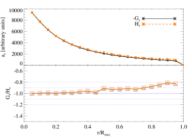
Figure 13: Hydrostatic sphere. Top panel: radial profiles of the ${\cal G}_{r}$ (changed in sign, for visualization and comparison purposes) and ${\cal H}_{r}$ components, as in the legend. Bottom panel: radial profile of the (mean and median) ${\cal G}_{r}/{\cal H}_{r}$ profile, both from the particle-based calculation (black trinagles and solid line) and from the two separate components profiles (orange squares and dot-dashed line). In both panels, symbols and lines indicate mean and median values, respectively.

As visible from the ${\cal G}_{r}$ (changed in sign) and ${\cal H}_{r}$ profiles in Figure 13 (upper panel), the HE configuration shows very good balance between the two components out to very large radii, with their ratio showing almost perfect balance in the central region ($\delta_{\rm HE}\lesssim 5\%$), and presenting deviations from HE smaller than 10% roughly out to $R_{\rm 200}$ ($\sim 1200\rm{\,kpc}$, i.e. $0.8\,R_{\rm max}$ in the Figure). In fact, from the inspection of the ${\cal G}_{r}/{\cal H}_{r}$ profile at different time-steps, till the final configuration shown in Figure 13 (lower panel), we observe a clear trend of the profile to set towards the -1 reference line, with the radial range in which the equilibrium condition is satisfied extending outwards. Given this, we expect that a perfect HE profile would be reached after an ideally large number of dynamical times. From the comparison with the various profiles obtained for the cosmological cases, presented in the previous sections, we estimate this effect not to cause any bias to the conclusions drawn from our study.

This study case is used to confirm that the HE, on the radial direction, corresponds indeed to ${\cal G}_{r}/{\cal H}_{r}\sim-1$, i.e. to the balance of the radial components of gravitational and hydrodynamical accelerations.

From the comparison in the Figure between the profiles of ${\cal G}_{r}$, ${\cal H}_{r}$ and ${\cal G}_{r}/{\cal H}_{r}$, we additionally tested that:

1. the particle-based approach and the use of the separate profiles of ${\cal G}_{r}$ and ${\cal H}_{r}$ converge to the same result for an ideal hydrostatic gas distribution (perfect overlap between symbols (mean values) and lines (median values) in the lower panel);

2. mean and median values within the radial bins provide exactly the same result (perfect overlap between curves and symbols), given the absence of gas inhomogeneities.

References

- Applegate et al. (2015) Applegate, D. E., Mantz, A., Allen, S. W., von der Linden, A., Morris, R. G., Hilbert, S., Kelly, P. L., Burke, D. L., Ebeling, H., Rapetti, D. A., & Schmidt, R. W. 2015, ArXiv e-prints
- Beck et al. (2016) Beck, A. M., Murante, G., Arth, A., Remus, R.-S., Teklu, A. F., Donnert, J. M. F., Planelles, S., Beck, M. C., Förster, P., Imgrund, M., Dolag, K., & Borgani, S. 2016, MNRAS, 455, 2110
- Biffi et al. (2011) Biffi, V., Dolag, K., & Böhringer, H. 2011, MNRAS, 413, 573
- Biffi et al. (2013) —. 2013, MNRAS, 428, 1395
- Biffi et al. (2014) Biffi, V., Sembolini, F., De Petris, M., Valdarnini, R., Yepes, G., & Gottlöber, S. 2014, MNRAS, 439, 588
- Bonafede et al. (2011) Bonafede, A., Dolag, K., Stasyszyn, F., Murante, G., & Borgani, S. 2011, MNRAS, 418, 2234
- Donahue et al. (2014) Donahue, M., Voit, G. M., Mahdavi, A., Umetsu, K., Ettori, S., Merten, J., Postman, M., Hoffer, A., Baldi, A., Coe, D., Czakon, N., & et al. 2014, ApJ, 794, 136
- Ettori et al. (2013) Ettori, S., Pratt, G. W., de Plaa, J., Eckert, D., Nevalainen, J., Battistelli, E. S., Borgani, S., Croston, J. H., Finoguenov, A., Kaastra, J., Gaspari, M., Gastaldello, F., Gitti, M., Molendi, S., Pointecouteau, E., & et al. 2013, ArXiv e-prints
- Fang et al. (2009) Fang, T., Humphrey, P., & Buote, D. 2009, ApJ, 691, 1648
- Gaspari et al. (2015) Gaspari, M., Brighenti, F., & Temi, P. 2015, A&A, 579, A62
- Gaspari & Churazov (2013) Gaspari, M. & Churazov, E. 2013, A&A, 559, A78
- Gaspari et al. (2014) Gaspari, M., Churazov, E., Nagai, D., Lau, E. T., & Zhuravleva, I. 2014, A&A, 569, A67
- Jeltema et al. (2008) Jeltema, T. E., Hallman, E. J., Burns, J. O., & Motl, P. M. 2008, ApJ, 681, 167
- Kravtsov & Borgani (2012) Kravtsov, A. V. & Borgani, S. 2012, ARA&A, 50, 353
- Lau et al. (2009) Lau, E. T., Kravtsov, A. V., & Nagai, D. 2009, ApJ, 705, 1129
- Lau et al. (2013) Lau, E. T., Nagai, D., & Nelson, K. 2013, ApJ, 777, 151
- Mahdavi et al. (2013) Mahdavi, A., Hoekstra, H., Babul, A., Bildfell, C., Jeltema, T., & Henry, J. P. 2013, ApJ, 767, 116
- Mahdavi et al. (2008) Mahdavi, A., Hoekstra, H., Babul, A., & Henry, J. P. 2008, MNRAS, 384, 1567
- Mazzotta et al. (2004) Mazzotta, P., Rasia, E., Moscardini, L., & Tormen, G. 2004, MNRAS, 354, 10
- Meneghetti et al. (2010) Meneghetti, M., Rasia, E., Merten, J., Bellagamba, F., Ettori, S., Mazzotta, P., Dolag, K., & Marri, S. 2010, A&A, 514, A93
- Meneghetti et al. (2014) Meneghetti, M., Rasia, E., Vega, J., Merten, J., Postman, M., Yepes, G., & et al. 2014, ApJ, 797, 34
- Nandra et al. (2013) Nandra, K., Barret, D., Barcons, X., Fabian, A., den Herder, J.-W., Piro, L., Watson, M., Adami, C., Aird, J., Afonso, J. M., & et al. 2013, ArXiv e-prints
- Nelson et al. (2014) Nelson, K., Lau, E. T., Nagai, D., Rudd, D. H., & Yu, L. 2014, ApJ, 782, 107
- Nelson et al. (2012) Nelson, K., Rudd, D. H., Shaw, L., & Nagai, D. 2012, ApJ, 751, 121
- Neto et al. (2007) Neto, A. F., Gao, L., Bett, P., Cole, S., Navarro, J. F., Frenk, C. S., White, S. D. M., Springel, V., & Jenkins, A. 2007, MNRAS, 381, 1450
- Piffaretti & Valdarnini (2008) Piffaretti, R. & Valdarnini, R. 2008, A&A, 491, 71
- Planelles et al. (2014) Planelles, S., Borgani, S., Fabjan, D., Killedar, M., Murante, G., Granato, G. L., Ragone-Figueroa, C., & Dolag, K. 2014, MNRAS, 438, 195
- Rasia et al. (2015) Rasia, E., Borgani, S., Murante, G., Planelles, S., Beck, A. M., Biffi, V., Ragone-Figueroa, C., Granato, G. L., Steinborn, L. K., & Dolag, K. 2015, ApJ, 813, L17
- Rasia et al. (2006) Rasia, E., Ettori, S., Moscardini, L., Mazzotta, P., Borgani, S., Dolag, K., Tormen, G., Cheng, L. M., & Diaferio, A. 2006, MNRAS, 369, 2013
- Rasia et al. (2014) Rasia, E., Lau, E. T., Borgani, S., Nagai, D., Dolag, K., Avestruz, C., Granato, G. L., Mazzotta, P., Murante, G., Nelson, K., & Ragone-Figueroa, C. 2014, ApJ, 791, 96
- Rasia et al. (2004) Rasia, E., Tormen, G., & Moscardini, L. 2004, MNRAS, 351, 237
- Rossetti et al. (2011) Rossetti, M., Eckert, D., Cavalleri, B. M., Molendi, S., Gastaldello, F., & Ghizzardi, S. 2011, A&A, 532, A123
- Sereno & Ettori (2015) Sereno, M. & Ettori, S. 2015, MNRAS, 450, 3633
- Shi et al. (2015) Shi, X., Komatsu, E., Nagai, D., & Lau, E. T. 2015, ArXiv e-prints
- Simet et al. (2015) Simet, M., Battaglia, N., Mandelbaum, R., & Seljak, U. 2015, ArXiv e-prints
- Smith et al. (2016) Smith, G. P., Mazzotta, P., Okabe, N., Ziparo, F., Mulroy, S. L., Babul, A., Finoguenov, A., McCarthy, I. G., Lieu, M., Bahé, Y. M., Bourdin, H., Evrard, A. E., Futamase, T., Haines, C. P., Jauzac, M., Marrone, D. P., Martino, R., May, P. E., Taylor, J. E., & Umetsu, K. 2016, MNRAS, 456, L74
- Springel (2005) Springel, V. 2005, MNRAS, 364, 1105
- Springel & Hernquist (2003) Springel, V. & Hernquist, L. 2003, MNRAS, 339, 289
- Steinborn et al. (2015) Steinborn, L. K., Dolag, K., Hirschmann, M., Prieto, M. A., & Remus, R.-S. 2015, MNRAS, 448, 1504
- Suto et al. (2013) Suto, D., Kawahara, H., Kitayama, T., Sasaki, S., Suto, Y., & Cen, R. 2013, ApJ, 767, 79
- Tornatore et al. (2007) Tornatore, L., Borgani, S., Dolag, K., & Matteucci, F. 2007, MNRAS, 382, 1050
- Tornatore et al. (2004) Tornatore, L., Borgani, S., Matteucci, F., Recchi, S., & Tozzi, P. 2004, MNRAS, 349, L19
- Vazza et al. (2009) Vazza, F., Brunetti, G., Kritsuk, A., Wagner, R., Gheller, C., & Norman, M. 2009, A&A, 504, 33
- von der Linden et al. (2014) von der Linden, A., Mantz, A., Allen, S. W., Applegate, D. E., Kelly, P. L., Morris, R. G., Wright, A., Allen, M. T., Burchat, P. R., Burke, D. L., Donovan, D., & Ebeling, H. 2014, MNRAS, 443, 1973