On the detectability of CO molecules in the Interstellar Medium via X-ray spectroscopy

Abstract

We present a study of the detectability of CO molecules in the Galactic interstellar medium using high-resolution X-ray spectra obtained with the XMM-Newton Reflection Grating Spectrometer. We analyzed 10 bright low mass X-ray binaries (LMXBs) to study the CO contribution in their line-of-sights. A total of 25 observations were fitted with the ISMabs X-ray absorption model which includes photoabsorption cross-sections for O I, O II, O III and CO. We performed a Monte-Carlo (MC) simulation analysis of the goodness of fit in order to estimate the significance of the CO detection. We determine that the statistical analysis prevents a significant detection of CO molecular X-ray absorption features, except for the lines-of-sight toward XTE J1718-330 and 4U 1636-53. In the case of XTE J1817-330, this is the first report of the presence of CO along its line-of-sight. Our results reinforce the conclusion that molecules have a minor contribution to the absorption features in the O K-edge spectral region. We estimate a CO column density lower limit to perform a significant detection with XMM-Newton of $N({\rm CO})>6$ $\times 10^{16}$ cm^-2 for typical exposure times.

1 Introduction

The physical conditions in the interstellar medium (ISM) can be studied through the technique of high-resolution X-ray spectroscopy. Using a bright astrophysical X-ray source as a background lamp, one can analyze the absorption features that are imprinted in the spectra by the ISM material located between the observer and the source. Due to their high energy, X-ray photons interact not only with the atomic phase but also with molecules and dust. In this way, high-resolution X-ray spectra provide a powerful method to study basic properties of the ISM such as composition, degree of ionization, column densities, and elemental abundances.

The cold phase of the ISM is composed mostly of molecular gas, predominantly molecular hydrogen. However, there are no transitions in the H₂ molecule that can be excited at low temperatures, and thus other tracers need to be employed. Carbon monoxide (CO) is the next most abundant molecule (Wilson et al., 1970) in the ISM. The CO molecule can give rise to characteristic X-ray absorption features the oxygen K-edge region (21-24Å).

Multiple studies have been performed reporting the presence of multiple phases in the ISM using low mass X-ray binaries (LMXBs) as X-ray sources (Juett et al., 2004; Juett et al., 2006; Pinto et al., 2010, 2013; Liao et al., 2013; Luo & Fang, 2014). Regarding the molecular contribution to the spectra, Pinto et al. (2010) searched for CO molecular absorption by analyzing the XMM-Newton spectrum of the LMXB GS 1826-238, finding an upper limit for the CO column density of $<0.4\times 10^{17}$cm^-2. In a similar way, Pinto et al. (2013) analyzed the local ISM in the lines-of-sight toward nine LMXBs, reporting CO column densities of $0.02-0.7\times 10^{17}$cm^-2. However, an adequate modeling of the atomic component is imperative before trying to model the contribution due to molecules or dust. In this sense, Gatuzz et al. (2013a, b); Gatuzz et al. (2014, 2015) and Gatuzz et al. (2016) have conducted a sequential analysis of the galactic ISM using high-resolution X-ray spectra obtained with Chandra and XMM-Newton observatories, finding a satisfactory modeling of the O K-edge region using only atomic and ionic absorbers.

In this paper we present a study of the detectability of CO molecules in the ISM by analyzing the XMM-Newton spectra of 10 bright LMXBS. In modeling these spectra, we use the most-up-to date atomic data for atomic oxygen in combination with experimental measurements of CO photoabsorption cross-section (Barrus et al., 1979). The outline of this paper is as follows. In Section 2 we describe the reduction of the observational data. In Section 3 we describe the O K-edge model which is used to fit the spectra, and provide details concerning the atomic and molecular database. In Section 4 we discuss in detail the main results. Section 5 is dedicated to compare our results with previous works. Finally, in Section 6 we summarize our main conclusions.

Table 1: XMM-Newton observation list.

Source	ObsID	Obs. Date	Exposure	Galactic	Distance	$N({\rm H})$
			(ks)	coordinates	(kpc)	$10^{21}$cm-2
4U 1254–69	0060740101	22-01-2001	$17.58$	$(303.48;-6.42)$	$13.0\pm 3.0^{a}$	$2.15$
	0060740901	08-02-2002	$29.62$
	0405510301	13-09-2006	$61.32$
	0405510401	14-01-2007	$62.91$
	0405510501	09-03-2007	$61.32$
4U 1543–62	0061140201	05-02-2001	$50.10$	$(321.76;-6.34)$	$7.0^{b}$	$2.46$
4U 1636–53	0500350301	29-09-2007	$31.94$	$(332.92;-4.82)$	$6.0\pm 0.5^{c}$	$2.64$
	0500350401	27-02-2008	$39.94$
	0606070101	15-03-2009	$41.18$
	0606070301	05-09-2009	$43.20$
4U 1735–44	0090340201	03-09-2001	$21.77$	$(346.0;-6.9)$	$9.4\pm 1.4^{d}$	$2.56$
	0090340601	01-04-2013	$85.00$
Cygnus X–2	0111360101	03-06-2002	$21.54$	$(87.33;-11.32)$	$13.4\pm 2.0^{d}$	$1.88$
	0303280101	14-06-2005	$31.81$
GRO J1655–40	0112921401	14-03-2005	$15.62$	$(344.98;2.46)$	$3.2\pm 0.2^{d}$	$5.78$
	0112921501	15-03-2005	$15.62$
	0112921601	16-03-2005	$15.61$
GS 1826–238	0150390101	08-04-2003	$107.85$	$(9.27;-6.09)$	$6.7^{c}$	$1.68$
	0150390301	09-04-2003	$91.92$
GX 9+9	0090340101	04-09-2001	$20.06$	$(8.51;9.04)$	$4.4^{e}$	$1.98$
	0090340601	25-09-2002	$23.85$
	0694860301	28-03-2013	$36.58$
GX 339–4	0148220201	08-03-2003	$20.50$	$(338.94;-4.33)$	$10.0\pm 4.5^{f}$	$3.74$
	0148220301	20-03-2003	$16.27$
XTE J1817–330	0311590501	13-03-2006	$20.73$	$(359.8;-7.9)$	$2.5\pm 1.5^{g}$	$1.39$
Hydrogen column density values are obtained from Kalberla et al. (2005). (a)in’t Zand et al. (2003); (b) Wang & Chakrabarty (2004); (c) Galloway et al. (2006); (d) Jonker & Nelemans (2004); (e) Grimm et al. (2002); (f) Hynes et al. (2004); (g) Sala & Greiner (2006).

2 Observations and data reduction

We have analyzed 10 bright LMXBs spectra obtained with the XMM-Newton observatory. XMM-Newton carries two high spectral resolution instruments, the Reflection Grating Spectrometers (RGS; den Herder et al., 2001). Each RGS consists of an array of reflection gratings which allows the diffraction of the X-rays, which are then detected on the charge couple devices (CCDs). The maximum instrumental resolution is $\Delta\lambda\sim$ 0.06Å  with a maximum effective area of about 140 cm² around 15 Å. The pileup effect, the detection of two events simultaneously as one single event, does not affect the O K-edge absorption region (21–24Å), and thus it can be ignored. Table 1 shows the specifications of the sources analyzed, including hydrogen column density 21 cm measurements from the Kalberla et al. (2005) survey, while Figure 2 shows the location in Galactic coordinates of all these source. We have reduced the data with the Science Analysis System (SAS, version 14.0.0) using the standard procedure to obtain the RGS spectra. A total of 25 observations were analyzed. We use $\chi^{2}$ statistic with the weighting method for low counts regime defined by Churazov et al. (1996). The spectral fitting was performed with the xspec analysis data package (Arnaud, 1996, version 12.9.0e)

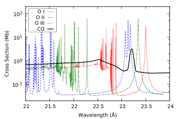
Figure 1: Photoionization cross-sections included on ISMabs for the O K-edge modeling. O I was computed by Gorczyca et al. (2013), while O II and O III were computed by García et al. (2005). The CO cross-section was measured experimentally by Barrus et al. (1979).

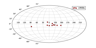
Figure 2: Aitoff projection of the location for all low mass X-ray binaries analyzed in this work.

3 O K-edge modeling

In order to model the O K-edge absorption region (21–24 Å) we used a simple power-law model for the continuum and the ISMabs X-ray absorption model which includes neutrally, singly, and doubly ionized species of H, He, C, N, O, Ne, Mg, Si, S, Ar and Ca (Gatuzz et al., 2015). We fixed the H column densities to the $N({\rm H})$ values reported by Gatuzz et al. (2016), which were obtained through a broadband fit (11–24 Å) for all sources included in the present work. In the case of 4U 1543–62, which was not included in the Gatuzz et al. (2016) analysis, we use the $N({\rm H})$ value from the 21 $cm$ measurements indicated in Table 1. For each source, we fitted all observation simultaneously using the same Photon-index as well as the column densities for O I, O II and O III, while allowing the normalization to vary. This accounts for the possibility of variability in the flux from the LMXB while maintaining the ISM absorption at a fixed value.

Table 2: O K-edge fit results.

Source	$N({\rm H})$	$N({\rm O~{}{\sc I}})$	$N({\rm O~{}{\sc II}})$	$N({\rm O~{}{\sc III}})$	$\chi^{2}$/dof	$\Delta\chi^{2}$	$N({\rm CO})$
	($10^{21}$cm-2)	($10^{17}$cm-2)	($10^{16}$cm-2)	($10^{16}$cm-2)		With CO	($10^{16}$cm-2)
4U 1254–69	$2.2$	$16.82\pm 14.29$	$3.67\pm 2.62$	$2.47\pm 2.06$	$1918/1762$	$<8$	–
4U 1543–62	$2.46$	$19.45\pm 2.04$	$6.38\pm 4.27$	$4.23\pm 3.67$	$275/291$	$<4$	–
4U 1636–53	$5.6$	$24.92\pm 1.35$	$8.73\pm 3.34$	$7.38\pm 4.05$	$1412/1181$	$<12$	$7.08\pm 3.45$
4U 1735-44	$3.2$	$19.98\pm 2.35$	$6.64\pm 2.27$	$5.52\pm 3.96$	$657/583$	$<7$	–
Cygnus X–2	$4.3$	$15.05\pm 0.68$	$6.65\pm 0.76$	$3.59\pm 2.18$	$709/588$	$<9$	–
GRO J1655–40	$7.8$	$32.47\pm 2.30$	$5.51\pm 2.87$	$3.45\pm 2.52$	$1042/882$	$<1$	–
GS 1826–238	$3.1$	$26.27\pm 1.99$	$5.85\pm 3.10$	$0.07\pm 0.05$	$671/590$	$<1$	–
GX 9+9	$7.4$	$18.73\pm 2.04$	$4.63\pm 4.29$	$3.92\pm 3.57$	$330/589$	$<3$	–
GX 339–4	$4.1$	$32.03\pm 2.11$	$8.79\pm 4.25$	$6.14\pm 3.04$	$671/592$	$<1$	–
XTE J1817-330	$1.4$	$13.18\pm 1.45$	$8.34\pm 3.69$	$4.50\pm 1.97$	$385/293$	$<12$	$7.22\pm 0.57$

The use of accurate atomic data is crucial to model the O K-edge absorption features (21–24Å). Owing to relaxation effects (Auger damping) the absorption K-edge does not have a simple edge shape but instead shows multiple resonances which lead to the smearing of the edge when viewed with an instrument with finite resolution (García et al., 2005). ISMabs includes O I cross-section from Gorczyca et al. (2013) and O II, O III cross-sections from García et al. (2005). These cross-sections have been improved by using astrophysical observations as reference for the energy position of the resonances, making them the best atomic data currently available for high-resolution X-ray spectroscopy analysis (Gatuzz et al., 2014, 2015).

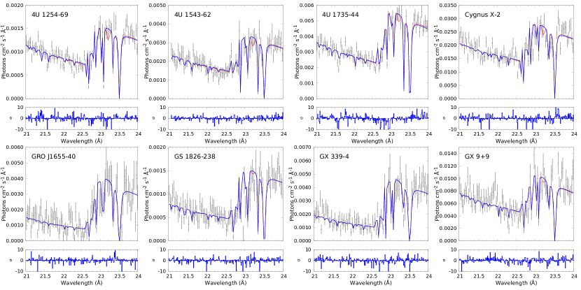
Figure 3: Oxygen K-edge region ISMabs best fits without CO (blue dotted lines) and including CO (red solid lines). For all sources above we can safely reject a successful detection of CO (see text for details).

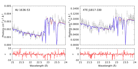
Figure 4: ISMabs best fit of the oxygen K-edge region without CO (blue solid lines) and including CO (red dotted lines). For both sources we obtained a significant CO detection with at least $95\%$ confidence.

After the best fit is found by using only an atomic component, we allow the CO column density to vary. In order to model the CO molecular absorption, we use the cross-section measured experimentally by Barrus et al. (1979). This cross section does not includes the measurements at the resonance. Instead, Barrus et al. (1979) estimated the peak intensities of the resonance based on measurements with different column densities (see their Table 4) and using these values we can obtain a complete cross section by joining them smoothly. A complete CO photoabsorption cross-section has been incorporated in the spex data analysis package and we have made use of it. Figure 1 shows the cross-sections included on ISMabs in order to model the O K-edge. The principal CO resonance, located at $\sim$23.20 Å, corresponds to the excitation to the 2$p\pi^{*}$ orbital and ${}^{1}\Pi$ state with a high width, compared with the O I, O II and O III resonances, attributed to the vibrational level excitation. In that respect, Barrus et al. (1979) quoted an uncertainty in the energy scale for the measurements of $\pm$ $0.3$ eV ($\pm$ 0.026 Å) while theoretical analysis of molecular vibrational modes indicate a vibrational spacing $<0.14$ eV ($<0.012$ Å) (Domke et al., 1990). Finally, this strong feature is partially embedded in the O III K$\alpha$ triplet, making difficult its detection.

Figure 5: Monte-Carlo simulation analysis to estimate the significance of the detection of the CO absorption feature. Vertical dashed lines correspond to the best $\chi^{2}$ obtained for each source.

4 Results and discussions

Table 2 shows the results from the best fits for all sources analyzed. As was detailed on Section 3, first we performed a fit allowing the O I, O II and O III column densities to vary as well as the powerlaw parameters. After obtain the best fit, we allow the CO column density to vary, as well as the O column densities, until we obtain the best fit. $\Delta\chi^{2}$ values on Table 2 correspond to the statistical difference, in units of $\chi^{2}$, between the model without CO and the model including CO. The largest increases in the statistic correspond to the objects 4U 1636-53 and XTE J1817-330 (both with $\Delta\chi^{2}<12$).

Figures 3 and 4 show the best fit of our model to the O K-edge region for all the sources selected. Observations for the same source are combined for illustrative purposes only. Figure 3 shows those sources for which the CO absorption feature has not been statistically detected, while Figure 4 shows the two sources for which a successful CO detection has been performed (see explanation below). In general, the residuals obtained without the CO contribution are small and evenly distributed along the wavelength region, indicating satisfactory modeling only with an atomic model. This is reflected in the fit statistics which correspond, in all cases, to $\chi^{2}/dof\sim 1$ (see Table 2). For sources in which the inclusion of CO yielded to some improvement in the fit statistics, the presence of the CO resonance at $23.20$Å can be appreciated in the models shown in Figures 3 and 4. However, in most cases the statistical improvement –referring to the variation on the $\chi^{2}$ value– is low.

We have performed a Monte-Carlo (MC) simulation analysis of the goodness of fit in order to estimate the significance of the CO detection for all sources with $\Delta\chi^{2}>2$. First, we fit the spectra with the reference model (i.e. ISMabs* powerlaw, without including CO), obtaining a $\chi^{2}$ statistical value. Second, we allow the CO component to vary, obtaining a second $\chi^{2}$ statistical value. This procedure was performed $10^{4}$ times by generating synthetic spectra for the source and background with the same exposure times as the combined data. Each fake spectrum (i.e. without CO) was fitted with a model which include CO as free parameter and the $\chi^{2}$ value was recorded. Following this procedure, the number of simulations where the reduction in the $\chi^{2}$ is at least as large as the observed in the real fit relative to the total number of simulations gives the probability of a false detection.

Figure 5 shows the MC results for the sources with $\Delta\chi^{2}>2$. Vertical dashed lines correspond to the $\chi^{2}$ value for the best fit model including CO. Table 3 shows false detection probability values derived from the MC simulations. We computed the significance of the CO possible detection in units of $\sigma$. Finally, the minimum $\sigma$ units required to ensure a $95\%$ significant detection is included for each case. This last value depends on the degrees of freedom involved, i.e., the number of free parameters in the O K-edge fit, which are also indicated in Table 3.

Table 3: Monte-Carlo analysis.

Source	d.o.f.	$\rho^{a}$	$\sigma^{b}$	Significant
				Regimec
4U 1254–69	3	$99.69$	$<0.35$	$3.84$
4U 1543–62	8	$78.52$	$<4.59$	$15.51$
4U 1735-44	4	$13.46$	$<7.78$	$9.49$
Cygnus X–2	4	$10.87$	$<7.78$	$9.49$
GX 9+9	5	$10.08$	$<9.24$	$11.07$
4U 1636–53	6	$3$	$<6.64$	$3.84$
XTE J1817-330	3	$2$	$<6.64$	$3.84$
(a) False detection probability (in $\%$); (b) Significance of the possible CO detection (in $\sigma$ units); (c) Minimum $\sigma$ required to ensure a $95\%$ significant detection.

For 4U 1254–69, 4U 1543–62, 4U 1735-44, Cygnus X–2, and GX 9+9 we obtained a false detection probability of $>10\%$, and therefore we can safely reject a successful detection of CO toward these lines-of-sight. On the other hand, we obtained a false detection probability of $3\%$ and $2\%$ in 4U 1636–53 and XTE J1817-330, respectively. These values correspond to a significant detection with at least $95\%$ confidence. The column density value measured are $N({\rm CO})=(7.22\pm 0.57)$ $\times 10^{16}$cm^-2 (for XTE J1817-330) and $N({\rm CO})=(7.08\pm 3.45)$ $\times 10^{16}$cm^-2 (for 4U 1636–53).

5 Comparison with Previous Work

Pinto et al. (2010) modeled the LMXB GS 1826–238 XMM-Newton high-resolution spectra using the spex analysis software, which includes the molecular absorption model (amol). They found an upper limit for the CO column density of $<4.0\times 10^{16}$cm^-2, as well as upper limits for Ca₃Fe₂Si₃O₁₂, amorphous ice (H₂O), carbon monoxide (CO), and hercynite (FeAl₂O₄) column densities. Pinto et al. (2013) also report the detection of CO analyzing nine LMXBs, six of which are included in this work. The CO column density values vary between $0.02-0.7\times 10^{17}$ cm^-2 along the multiple lines-of-sight. In the case of 4U 1636–53, they estimate a column density of $N({\rm CO})=(3.0\pm 2.0)$ $\times 10^{16}$ cm^-2. However, the O I, O II, and O III atomic cross sections incorporated in the spex models do not include the effects of Auger damping, which has a significant effect in the structure of the K-edge. This limits the ability of these models to reproduce the observations.

On the other hand, our findings are consistent with those of Gatuzz et al. (2013a, b), who achieved good O K-edge fits to Chandra high-resolution spectra using a warmabs model based on the xstar photoionization code, without clear evidence for the presence of CO X-ray absorption features. More recently, Gatuzz et al. (2016) have performed a comprehensive analysis of the ISM along 24 lines of sight using both Chandra and XMM-Newton high-resolution spectra, demonstrating statistically acceptable fits without molecular or solid contribution to the absorption in the O K-edge wavelength region.

Large-scale CO surveys show that CO is the dominant molecule in the interstellar medium, after $H_{2}$, and that its abundance relative to $H_{2}$ is $\sim 10^{-4}$, i.e. most oxygen is bound in the molecule in the cold phase of the ISM (Herbst & Klemperer, 1973). The major contribution of CO in the Milky Way is expected to be in the Galactic plane, with higher CO column densities around the galactic center (Bitran et al., 1997; Dame et al., 2001; Nakanishi & Sofue, 2006; Padoan et al., 2006; Pettitt et al., 2015). However, the Galactic extinction toward these lines-of-sight makes it difficult to obtain spectra which are well suited to the study of the O K-edge region. Therefore, the sources included in our sample satisfy (1) line-of-sight toward or near the galactic plane, and (2) high counts rate in the 21–24 Å wavelength region, allowing the modeling not only of O I K$\alpha$, but also O II and O III K$\alpha$ lines. However, according to the survey of Dame et al. (2001), the presence of CO in the line of sight toward our sample is predicted to be low, with an average value of $\sim 3.5\times 10^{16}$ cm^-2 for $|l|<10$. Using XMM-Newton response files we simulated spectra assuming typical O I, O II, and O III column densities measured by Gatuzz et al. (2016), and a typical exposure time (e.g. 30 ks) in order to determine the minimum CO column density required to perform a successful detection. We found a lower limit value corresponding to $N({\rm CO})>6$ $\times 10^{16}$ cm^-2. In the case of Chandra we found a lower limit value to perform a significant detection of $N({\rm CO})>12$ $\times 10^{16}$ cm^-2. These values are comparable to the upper limits and detections that we report in the previous section.

The presence of CO along the line-of-sight toward XTE–J1817-330 has not been reported before. XTE–J1817-330 constitutes a bright source with high signal-to-noise ratio in the O K-edge wavelength region to allow the identification of K$\beta$ and K$\gamma$ O I absorption lines (Gatuzz et al., 2013a, b). The quality of the spectra is reflected in the error bar of the CO column density, which correspond to a $7\%$ of the measured value. In the case of 4U 1636–53, we agree with CO column density estimated by Pinto et al. (2013). However, it should be noted that the error for the CO column density in our modeling is large enough that our measurement should be taken as an upper limit.

6 Conclusions

We reported on the spectral analysis of 10 Galactic X-ray binaries located in the Galactic plane and the search for CO X-ray absorption features in these spectra. A total of 25 XMM-Newton observations were analyzed. We modeled the O K-edge absorption region (21–24 Å) using the ISMabs X-ray absorption model, which includes singly, and doubly ionized photoabsorption cross-sections for O. For all sources we were able to asses the presence and strength of O I, O II, and O III absorption features, measuring the column density for each ion. We include the CO experimental photo-absorption cross section measured by Barrus et al. (1979) in order to model the contribution of CO to the absorption spectra. We performed Monte-Carlo simulations to obtain a rigorous estimate of the statistical significance of possible CO detection concluding that the statistical analysis prevents from a significant detection of CO molecular X-ray absorption features in 8 of the sources analyzed. Finally, we measured CO column density values for XTE–J1817-330 ($7.22\pm 0.57$ $\times 10^{16}$ cm^-2), and 4U 1636-53 ($7.08\pm 3.45$ $\times 10^{16}$ cm^-2). This, along with simulations, suggests that the statistical quality of the current archive of XMM-Newton RGS observations is generally not sufficient to detect CO from a large fraction of the sight lines which have been observed. The detections likely represent sight lines with columns greater than average. Deeper observations with the existing instruments have the potential to detect CO along more lines of sight.

References

- Arnaud (1996) Arnaud K. A., 1996, in Jacoby G. H., Barnes J., eds, Astronomical Society of the Pacific Conference Series Vol. 101, Astronomical Data Analysis Software and Systems V. p. 17
- Barrus et al. (1979) Barrus D. M., Blake R. L., Burek A. J., Chambers K. C., Pregenzer A. L., 1979, Phys. Rev. A, 20, 1045
- Bitran et al. (1997) Bitran M., Alvarez H., Bronfman L., May J., Thaddeus P., 1997, A&AS, 125
- Churazov et al. (1996) Churazov E., Gilfanov M., Forman W., Jones C., 1996, ApJ, 471, 673
- Dame et al. (2001) Dame T. M., Hartmann D., Thaddeus P., 2001, ApJ, 547, 792
- Domke et al. (1990) Domke M., Xue C., Puschmann A., Mandel T., Hudson E., Shirley D. A., Kaindl G., 1990, Chemical Physics Letters, 173, 122
- Galloway et al. (2006) Galloway D. K., Psaltis D., Muno M. P., Chakrabarty D., 2006, The Astrophysical Journal Letters, 639, 1033
- García et al. (2005) García J., Mendoza C., Bautista M. A., Gorczyca T. W., Kallman T. R., Palmeri P., 2005, ApJS, 158, 68
- Gatuzz et al. (2013a) Gatuzz E., et al., 2013a, ApJ, 768, 60
- Gatuzz et al. (2013b) Gatuzz E., et al., 2013b, ApJ, 778, 83
- Gatuzz et al. (2014) Gatuzz E., García J., Mendoza C., Kallman T. R., Bautista M. A., Gorczyca T. W., 2014, ApJ, 790, 131
- Gatuzz et al. (2015) Gatuzz E., García J., Kallman T. R., Mendoza C., Gorczyca T. W., 2015, ApJ, 800, 29
- Gatuzz et al. (2016) Gatuzz E., García J. A., Kallman T. R., Mendoza C., 2016, preprint, (arXiv:1602.06955)
- Gorczyca et al. (2013) Gorczyca T. W., et al., 2013, ApJ, 779, 78
- Grimm et al. (2002) Grimm H.-J., Gilfanov M., Sunyaev R., 2002, A&A, 391, 923
- Herbst & Klemperer (1973) Herbst E., Klemperer W., 1973, ApJ, 185, 505
- Hynes et al. (2004) Hynes R. I., Steeghs D., Casares J., Charles P. A., O’Brien K., 2004, ApJ, 609, 317
- Jonker & Nelemans (2004) Jonker P. G., Nelemans G., 2004, MNRAS, 354, 355
- Juett et al. (2004) Juett A. M., Schulz N. S., Chakrabarty D., 2004, ApJ, 612, 308
- Juett et al. (2006) Juett A. M., Schulz N. S., Chakrabarty D., Gorczyca T. W., 2006, ApJ, 648, 1066
- Kalberla et al. (2005) Kalberla P. M. W., Burton W. B., Hartmann D., Arnal E. M., Bajaja E., Morras R., Pöppel W. G. L., 2005, A&A, 440, 775
- Liao et al. (2013) Liao J.-Y., Zhang S.-N., Yao Y., 2013, ApJ, 774, 116
- Luo & Fang (2014) Luo Y., Fang T., 2014, ApJ, 780, 170
- Nakanishi & Sofue (2006) Nakanishi H., Sofue Y., 2006, PASJ, 58, 847
- Padoan et al. (2006) Padoan P., Cambrésy L., Juvela M., Kritsuk A., Langer W. D., Norman M. L., 2006, ApJ, 649, 807
- Pettitt et al. (2015) Pettitt A. R., Dobbs C. L., Acreman D. M., Bate M. R., 2015, MNRAS, 449, 3911
- Pinto et al. (2010) Pinto C., Kaastra J. S., Costantini E., Verbunt F., 2010, A&A, 521, A79
- Pinto et al. (2013) Pinto C., Kaastra J. S., Costantini E., de Vries C., 2013, A&A, 551, A25
- Sala & Greiner (2006) Sala G., Greiner J., 2006, The Astronomer’s Telegram, 791, 1
- Wang & Chakrabarty (2004) Wang Z., Chakrabarty D., 2004, ApJ, 616, L139
- Wilson et al. (1970) Wilson R. W., Jefferts K. B., Penzias A. A., 1970, ApJ, 161, L43
- den Herder et al. (2001) den Herder J. W., et al., 2001, A&A, 365, L7
- in’t Zand et al. (2003) in’t Zand J. J. M., Kuulkers E., Verbunt F., Heise J., Cornelisse R., 2003, A&A, 411, L487