Exponential Orthogonality Catastrophe at the Anderson Metal-Insulator Transition

Abstract

We consider the orthogonality catastrophe at the Anderson Metal-Insulator transition (AMIT). The typical overlap $F$ between the ground state of a Fermi liquid and the one of the same system with an added potential impurity is found to decay at the AMIT exponentially with system size $L$ as $F\sim\exp(-\langle I_{A}\rangle/2)=\exp(-cL^{\eta})$, where $I_{A}$ is the so called Anderson integral, $\eta$ is the power of multifractal intensity correlations and $\langle...\rangle$ denotes the ensemble average. Thus, strong disorder typically increases the sensitivity of a system to an additional impurity exponentially. We recover on the metallic side of the transition Anderson’s result that fidelity $F$ decays with a power law $F\sim L^{-q(E_{F})}$ with system size $L$. This power increases as Fermi energy $E_{F}$ approaches mobility edge $E_{M}$ as $q(E_{F})\sim(\frac{E_{F}-E_{M}}{E_{M}})^{-\nu\eta},$ where $\nu$ is the critical exponent of correlation length $\xi_{c}$. On the insulating side of the transition $F$ is constant for system sizes exceeding localization length $\xi$. While these results are obtained from the mean value of $I_{A},$ giving the typical fidelity $F$, we find that $I_{A}$ is widely, log normally, distributed with a width diverging at the AMIT. As a consequence, the mean value of fidelity $F$ converges to one at the AMIT, in strong contrast to its typical value which converges to zero exponentially fast with system size $L$. This counterintuitive behavior is explained as a manifestation of multifractality at the AMIT.

Anderson showed in Ref. ao, that the addition of a static potential impurity to a system of N fermions changes its groundstate such that the overlap between the original $\langle\psi\mid$ and the new ground state $\langle\psi^{\prime}\mid$ has an upper bound,

$$\chi=F^{2}=|\langle\psi\mid\psi^{\prime}\rangle|^{2}<\exp\left(-I_{A}\right),$$ (1)

where the Anderson integral $I_{A}$ is for noninteracting electrons given in terms of the single particle eigenstates of the original system $|n\rangle$ and the new system $|m^{\prime}\rangle$ by

$$I_{A}=\frac{1}{2}\sum_{\epsilon_{n}\leq 0,\epsilon_{m^{\prime}}>0}|\langle n|m^{\prime}\rangle|^{2}.$$ (2)

If the added impurity is short ranged and of strength $\lambda$, Anderson found for a clean metal $I_{A}=2\pi^{2}\lambda^{2}\ln N,$ diverging with the number of fermions $N$, so that $F$, also called fidelity, decays with a power law with $N,$ leading to the so called orthogonality catastrophe (AOC). This implies that the local perturbation connects the system to a macroscpic number of excited states which has important consequences like the singularities in the X-Ray absorption and emission of metalsnozieresdominicis . Furthermore, the zero bias anomaly in disordered metalsaltshuleraronov and anomalies in the tunneling density of states in quantum Hall systemstunnelingDOS are related to the AOC The concept of fidelity can be generalised to any parametric perturbation of a system and be used to characterise quantum phase transitions venuti . The AOC has been explored in mesoscopic systemsmeso1 ; meso2 . With the advent of engineered many-body systems in ensembles of ultracold atoms it is possible to study nonequilibrium quantum dynamics of such systems in a controlled way so that conseuqences of parameter changes become measurable directlydemler .

An intriguing question is, if the system becomes less or more sensitive to the addition of another impurity if it already contains a finite density of impurities. Gefen et al. showed in Ref. gefenlerner, that in a weakly disordered metal the average value $\langle I_{A}\rangle$ scales with $\ln N$ when the potential of the added impurity potential is short ranged. That result is valid to leading order in $1/g,$ where $g=k_{\rm F}l_{e}\gg 1$ is a measure of disorder strength with mean free path $l_{e}$. Numerical results gefenlerner show that in a 2-dimensional disordered system $I_{A}$ increases as the disorder strength increases until it is so strong that localization length $\xi$ is smaller than system size $L$. Beyond that, $I_{A}$ decreases as $\xi$ decreases with increasing disorder. Thus, the addition of an impurity changes the ground state of weakly disordered systems more strongly than the one of a clean system. Only at strong disorder when the fermions are localized, its sensitivity to a potential change decreases again.

Here, we aim to derive this behavior analytically in order to find out how fidelity $F$ changes when tuning disorder strength or energy. In systems close to the Anderson metal-insulator transition (AMIT) we can use the fact that the single particle wavefunctions at the AMIT are multifractal multifractal and power law correlatedpowerlaw ; cuevas ; ioffe . We also obtain analytical results for noncritical 2-dimensional disordered systems, which confirm the numerical calculations of Ref. gefenlerner, . For a short range impurity of strength $\lambda$, located at position ${\bf x},$ $I_{A}$ can be expressed in terms of the local intensities of the unperturbed Eigenstates $|n>$ with Eigenenergies $E_{n},$ ao ; gefenlerner

$$I_{A}=\frac{(2\pi\lambda)^{2}}{2\rho^{2}}\sum_{E_{n}<E_{F}}\sum_{E_{m}>E_{F}}\frac{|\psi_{n}({\bf x})|^{2}|\psi_{m}({\bf x})|^{2}}{(E_{n}-E_{m})^{2}},$$ (3)

where $\rho$ is the mean density of states. The correlation function of the intensities associated to two energy levels distant by $\omega_{nm}=E_{n}-E_{m}$ is given by cuevas ; ioffe ; ioffe2

$$C(\omega_{nm}=E_{n}-E_{m})=L^{d}\int d^{d}r\,\left\langle|\psi_{n}({\bf r})|^{2}|\psi_{m}({\bf r})|^{2}\right\rangle$$

$$=\left\{\begin{array}[]{ll}(\frac{E_{c}}{{\rm Max}(|\omega_{nm}|,\Delta)})^{\eta/d},&0<|\omega_{nm}|<E_{c},\\ (E_{c}/|\omega_{nm}|)^{2},&|\omega_{nm}|>E_{c},\end{array}\right.,$$ (6)

when $E_{n}\leq E_{M}$ and $E_{m}\geq E_{M}$ or vice versakats . $\Delta=1/(\rho L^{d})$ is the average level spacing. Here, $\eta=2(\alpha_{0}-d)$, with multifractality parameter $\alpha_{0}$ and $d$ the dimension. The correlation energy $E_{c}$ is a macroscopic energy of order of elastic scattering rate $1/\tau$. For $|\omega_{nm}|<E_{c}$ correlations are enhanced in comparison to the plane-wave limit $C_{nm}=1$, see Fig. 1, where we set one of the energies at he mobility edge $E_{n}=E_{M}$ and the other at $E_{m}=E$. Note, that for $|\omega_{nm}|>E_{c}$ it decays below $1$. This anticorrelation ensures that the total intensity at a position ${\bf x}$ is normalised: A dip in intensity at one energy implies an enhancement of intensity at another energy and vice versa.

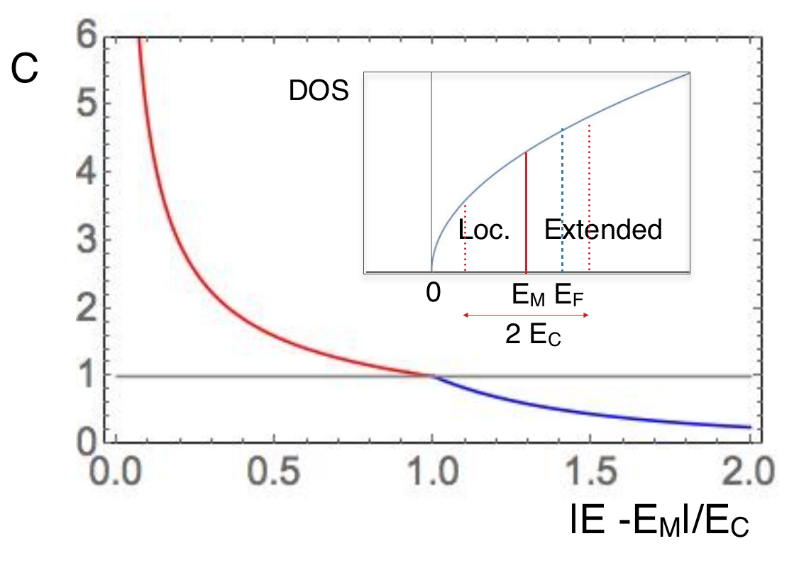
Figure 1: Correlation function of intensities $C$ as function of their energy difference $|E-E_{M}|$ in a disordered system with $\eta=2,d=2$. Inset: Density of states (DOS) as function of energy $E$ with a transition between localized and extended states at mobility edge $E_{M}$. Intensities are correlated within an energy window $2E_{c}$ around $E_{M}$.

Mean Value of the Anderson Integral.— Inserting Eq. (Exponential Orthogonality Catastrophe at the Anderson Metal-Insulator Transition) into Eq. (3), the average mean value of $I_{A}$ is

$$\langle I_{A}\rangle=\frac{(2\pi\lambda)^{2}}{2}\iint\limits_{\epsilon<-\Delta/2,\epsilon^{\prime}>\Delta/2}d\epsilon d\epsilon^{\prime}\frac{C_{\epsilon,\epsilon^{\prime}}}{(\epsilon-\epsilon^{\prime})^{2}}.$$ (7)

This gives the geometrical average of $F,$ $\exp(\langle\ln F\rangle)=\exp(-\langle I_{A}\rangle/2)$. At the AMIT we get with Eq. (Exponential Orthogonality Catastrophe at the Anderson Metal-Insulator Transition)

$$\langle I_{A}\rangle|_{E_{F}=E_{M}}=\frac{2(\pi\lambda)^{2}}{\gamma(1+\gamma)}\left(\frac{E_{c}}{\Delta}\right)^{\gamma},$$ (8)

diverging with number of particles $N=E_{F}/\Delta$ with a power law, $\gamma=\eta/d$.

As the Fermi energy is moved into the insulating regime $E_{F}<E_{M}$, there remain multifractal correlations, Eq. (Exponential Orthogonality Catastrophe at the Anderson Metal-Insulator Transition), but the integral is now cut off at local level spacing $\Delta_{\xi}=1/(\rho\xi^{d})$, since there is local level repulsionkats . This yields

$$\langle I_{A}\rangle|_{E_{F}<E_{M}}=\frac{2(\pi\lambda)^{2}}{\gamma(1+\gamma)}\left(\frac{E_{c}}{\Delta_{\xi}}\right)^{\gamma},$$ (9)

independent of the number of particles $N$.

In the metallic regime $E_{F}>E_{M}$ all wave functions are extended. On length scales smaller than correlation length $\xi_{c}$ multifractal fluctuations still occur and there are power-law correlations in energy Eq. (Exponential Orthogonality Catastrophe at the Anderson Metal-Insulator Transition). The energy difference $|\omega_{nm}|$ is for $\epsilon_{n}<\epsilon_{m}$ substituted by ${\rm Max}[|\omega_{nm}|,\Delta_{\xi_{cn}}]$, where $\Delta_{\xi_{cn}}=E_{c}\,(\xi_{cn}/a_{c})^{-d}$. $\xi_{cn}$ is the correlation length at energy $E_{n}$ and $a_{c}$ is a small length scale defined by $E_{c}=1/(\rho a_{c}^{d})$kats . For $\omega_{nm}<E_{c}$, correlations are enhanced in comparison to plane-wave limit $C_{nm}=1$, yielding

$$\langle I_{A}\rangle|_{E_{F}>E_{M}}=2(\pi\lambda)^{2}\left(\frac{E_{c}}{\Delta_{\xi_{c}}}\right)^{\gamma}\left(\frac{1}{\gamma(1+\gamma)}+\ln\frac{N}{N_{\xi_{c}}}\right),$$ (10)

diverging logarithmically with number of electrons $N$ in agreement with Anderson’s result for a metal, which is recovered exactly far away from the MIT, where $\Delta_{\xi_{c}}\rightarrow E_{c}$.

In Fig. 2 we plot the first moment of the Anderson Integral $\langle I_{A}\rangle$ as function of Fermi energy $E_{F}$ in units of mobility Edge $E_{M}$, Eqs. (8,9,10), for various system sizes L.

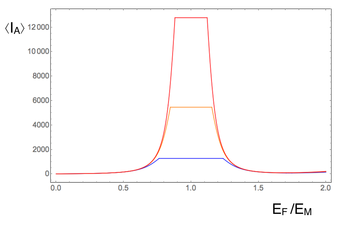
Figure 2: The average Anderson integral $\langle I_{A}\rangle$ as function of Fermi energy $E_{F}$ in units of mobility edge $E_{M}$ for a 3-dim. disordered system, Eqs. (8,9,10), for various system sizes $L$ (in units of microsopic length $a_{c}$), $L=10$ (blue), $L=20$ (orange) and $L=50$ (red).

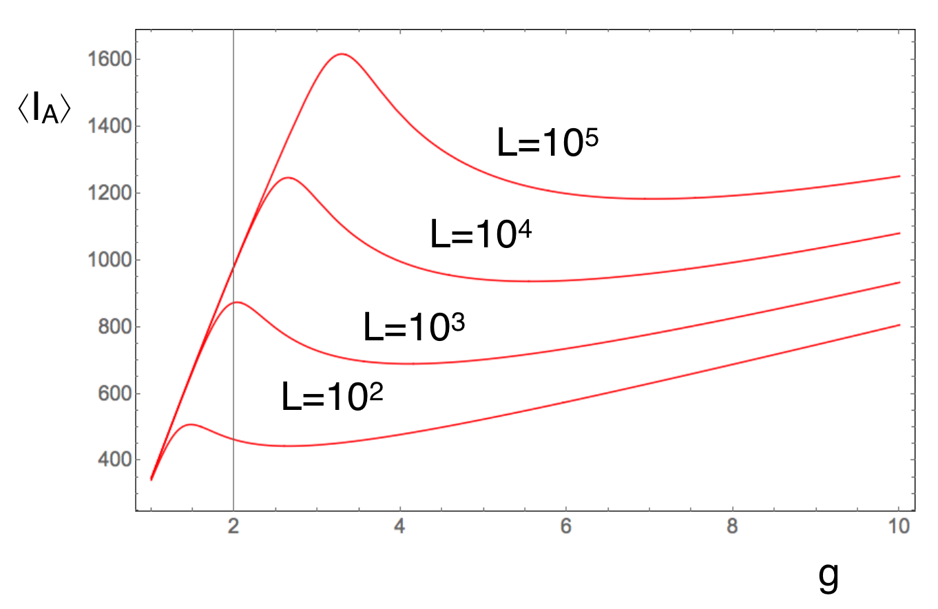
Figure 3: The average Anderson integral $\langle I_{A}\rangle$ as function of disorder paramter $g=E_{F}\tau$ for a 2-dimensional disordered system, as obtained by substituting $\xi_{2D}=g\exp(\pi g)$ and $\gamma_{2D}=1/(\pi g)$ into Eq. (9), with $\Delta_{\xi}=D/\xi^{2}$ and $\Delta=D/L^{2}$ for various system sizes $L$.

Anderson Integral of 2D Disordered Electon Systems.— In 2D disordered electron systems without spin-orbit interaction, without strong magnetic field and strong interactions all state are localized. Therefore, the Anderson integral is given by Eq. (9) with localization length $\xi_{2D}=g\exp(\pi g)$ (in units of the smallest microscopic length scale), where $g=\epsilon_{F}\tau$. In 2D weakly disordered systems, $g\gg 1,$ there are weak logarithmic correlations of the intensity at different energies which can to leading order in $1/g$ be written as power law correlations with power $\eta_{2D}=2/(\pi g)$. Substituting $\xi_{2D}$ and $\gamma_{2D}=1/(\pi g)$ into Eq. (9), with $\Delta_{\xi}=D/\xi^{2}$ and $\Delta=D/L^{2}$, where $D$ is the band width, we get the Anderson integral for 2D disordered systems as function of disorder paramter $g$ and system size $L$ as plotted in Fig. 3. We thus confirm analytically the nonomonotonous dependence of $\langle I_{A}\rangle$ as function of disorder strength as observed numerically in 2D disordered systems in Ref. gefenlerner, . We find that the maximal value of $I_{A}$ increases with system size logarithmically. When the localization length exceeds the system size $\xi>L$ we find $\langle I_{A}\rangle=2\pi(\pi\lambda)^{2}gL^{2/(\pi g)}$. Expanding in $1/g$ we recover to leading order Anderson’s result, $\langle I_{A}\rangle=const.+2(\pi\lambda)^{2}\ln L^{2}$. Note that the logarithmic divergence is independent of the disorder paramter $g$ and coincides exactly with Anderson’s result for a clean metal. In the opposite limit, when localization length $\xi$ is smaller than systems size $L$, we find $\langle I_{A}\rangle=2\pi(\pi\lambda)^{2}g\exp(2+2\ln g/(\pi g))$.

Distribution Function of the Anderson Integral.— Having obtained that the average Anderson integral diverges with the system size $L$ at the AMIT more strongly than in a clean or weakly disordered metal, we may ask how widely $I_{A}$ is distributed. Since it is a functional of the local density of states at the position where the additional impurity has been placed, Eq. (3), it is expected to be widely distributed. The distribution function of $I_{A}({\bf x})$ as obtained by placing the impurity in different ensembles with same disorder strength is

$$P(I_{A})=\int\prod_{l}d\alpha_{l}P\left(\{\alpha_{l}\}\right)\delta\left(I_{A}-I[\{\alpha_{l}\}]\right),$$ (11)

where $I[\{\alpha_{l}\}]$ is defined by the right side of Eq. (3). Following the strategy recently used in the derivation of the distribution function of Kondo temperatures $T_{K}$ at the AMITkats , we replace the correlated distribution function of all intensities $P\left(\{\alpha_{l}\}\right)$ by a product of pairwise joint distribution functions of $|\psi_{n}({\bf r}_{i})|^{2}$ and $|\psi_{m}({\bf r}_{i})|^{2}$, in accordance with the correlation function $C_{nm}$, Eq. (Exponential Orthogonality Catastrophe at the Anderson Metal-Insulator Transition). Thereby, we can derive the conditional intensity of a state at energy $E_{l}$, given that the intensity at mobility edge $E_{M}$ is $|\psi_{M}({\bf r})|^{2}=L^{-\alpha}$,kats

$$L^{d}\langle|\psi_{l}({\bf r})|^{2}\rangle_{|\psi_{M}({\bf r})|^{2}=L^{-\alpha}}=\left|\frac{E_{l}-E_{M}}{E_{c}}\right|^{r_{\alpha}},$$ (12)

where the power is given by $r_{\alpha}=\frac{\alpha-\alpha_{0}}{d}-\frac{\eta}{2d}g_{lM}$. When $E_{l}$ is located away from mobility edge $E_{M}$, the coefficient $g_{lM}=\ln|(E_{l}-E_{M})/E_{c}|/(d\ln L)$ vanishes for $L\rightarrow\infty$. Close to $E_{M}$ it saturates: $g_{lM}|_{E_{l}\rightarrow E_{M}}\rightarrow-1$ and Eq. (12) reduces to $L^{d-\alpha}$, the local intensity at $E_{M}$ relative to the intensity of an extended state $L^{-d}$kats . At positions where the local intensity at the mobility edge is small, corresponding to $\alpha>\alpha_{0}$, it is suppressed within an energy range of order $E_{c}$ around $E_{M},$ forming local pseudogaps with power $r_{\alpha}=\frac{\alpha-\alpha_{0}}{d}$. When the intensity at $E_{M}$ is larger than its typical value, $\alpha<\alpha_{0}$, there are local power law divergencies and the local density of states is enhanced within energy range $2E_{c}$ around $E_{M}$, increasing as a power law when $E_{l}$ approaches $E_{M}$.

Next, we can find the Anderson integral at a position ${\bf x}$, when the intensity of the state at the mobility edge $E_{n}=E_{M}$ at that position is fixed to $|\psi_{n}({\bf x})|^{2}=L^{-\alpha},$

$$\langle I_{A}\rangle_{\alpha}=2(\pi\lambda)^{2}\iint\limits_{\epsilon<-\Delta/2,\epsilon^{\prime}>\Delta/2}d\epsilon d\epsilon^{\prime}\frac{1}{(\epsilon-\epsilon^{\prime})^{2}}|\frac{\epsilon}{E_{c}}|^{r_{\alpha}}|\frac{\epsilon^{\prime}}{E_{c}}|^{r_{\alpha}}.$$ (13)

which yields

$$\langle I_{A}\rangle_{\alpha}=\frac{2(\pi\lambda)^{2}}{\gamma(1+\gamma)}\left(\frac{E_{c}}{D}\right)^{\gamma}L^{-2(\alpha-d)}.$$ (14)

Inverting this equation and inserting the result into the distribution function of $\alpha$, $P(\alpha)=\exp[-\ln L(\alpha-\alpha_{0})^{2}/(2\eta)]$ we get with Eq. (11),

$$P(I_{A})=\frac{1}{\sqrt{8\pi\eta\ln L}}\frac{1}{I_{A}}e^{-\frac{\left(\ln\frac{I_{A}}{\langle I_{A}\rangle}+2\eta\ln L\right)^{2}}{8\eta\ln L}},$$ (15)

where $\langle I_{A}\rangle$ is the first moment, Eq. (8). Thus, the Anderson integral is widely, log-normally distributed with a width which increases with system size $L$ logarithmically.

If the Fermi energy is in the insulating regime, $E_{F}<E_{M}$, there is multifractality on length scales smaller than localization length $\xi$ and the intensity scales with $\xi$, $|\psi_{l}({\bf x})|^{2}=\xi^{-\alpha_{l}}.$ Thus, we find the distribution function of $I_{A}$ by replacing the system size $L$ by $\xi$ in the above derivation at the MIT yielding Eq. (15), where $L$ is replaced by $\xi$.

On the metallic side of the transition all wave functions are extended and their intensities scale as $|\psi|^{2}\sim L^{-d}$. On length scales smaller than correlation length $\xi_{c}$ multifractal fluctuations of the wave function intensity occur as long as $\xi_{c}$ is larger than the microscopic length scale $a_{c}$.cuevas ; ioffe2 In the metallic phase, moments of intensity scale with $\xi_{c}$ as $L^{dq}\langle|\psi|^{2q}\rangle\sim\xi_{c}^{(d-d_{q})(q-1)}$ioffe2 ; mirlin ; kats . Therefore, we define $\alpha$ in the metal as $L^{d}|\psi_{l}({\bf r})|^{2}=\xi_{cl}^{d-\alpha_{l}}$, where $\xi_{cl}$ is the correlation length of state $l$. As the MIT is approached $\xi_{c}$ diverges and is replaced by system size $L$, so that $\alpha$ crosses over to the definition used above at the MIT. It has to a good approximation the Gaussian distribution, $P(\alpha_{l})\sim\exp[-\ln\xi_{cl}(\alpha_{l}-\alpha_{0})^{2}/(2\eta)]$ as confirmed numerically in Ref. kats, . Therefore, in deriving the distribution function of $I_{A},$ we can follow the strategy used at the MIT, deriving first the value of $I_{A}$ when averaged over all pair correlations, given that $\alpha$ at the Fermi energy is fixed,

$$\langle I_{A}\rangle_{\alpha}=2(\pi\lambda)^{2}c\left(\frac{1}{\gamma(1+\gamma)}+\ln\frac{N}{N_{\xi_{c}}}\right)\xi_{c}^{-2(\alpha-d)},$$ (16)

where $c=\left(E_{c}/D\right)^{\gamma}$. Inverting this equation and inserting it into the distribution function of $\alpha$ we get with Eq. (11) the distribution of $I_{A}$ in the metallic regime, Eq. (15), replacing $L$ by $\xi_{c}$ and $\langle I_{A}\rangle$ by the first moment Eq. (10).

We note that the first moment of $I_{A}$ yields the geometrical average of the fidelity $\exp(\langle\ln F\rangle)=\exp(-\langle I_{A}\rangle/2)$ giving a typical value of $F$. So far, we have not yet obtained the average fidelity $\langle F\rangle=\langle\exp(-I_{A}/2)\rangle$, since its calculation requires the knowledge of all moments of $I_{A}$ gefencomment . Using the distribution function as obtained in the pair approximation above, Eq. (15), we find at the AMIT

$$\langle F\rangle=\frac{1}{\sqrt{8\pi\eta\ln L}}\int_{-\infty}^{\infty}dxe^{-\langle I_{A}\rangle L^{-\eta}\exp(x)}e^{-\frac{x^{2}}{8\eta\ln L}}.$$ (17)

An expansion in moments of $I_{A}$ gives a divergent series. A saddle point approximation to the integral in Eq. (17), yields $\langle F\rangle|_{L\rightarrow\infty}=1,$ as confirmed by numerical integration, Fig. 4, where we plot $\langle F\rangle$, Eq. (17), as function of $\ln L.$

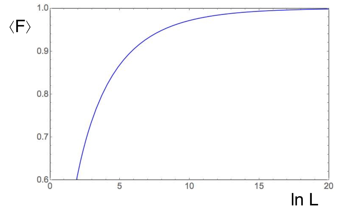
Figure 4: The average fidelity $\langle F\rangle$ as function of the logarithm of system size $L$ at the 3D AMIT for $\eta=2,$ $\lambda=1.$

We conclude that, typically, the Anderson orthogonality catastrophe becomes exponentially enhanced at the AMIT. The typical fidelity decays exponentially with system size $L$ as $F\sim\exp(-cL^{\eta})$, where $\eta$ is the power of multifractal intensity correlations. On the metallic side of the transition we recover Anderson’s result that the typical overlap decays with a power law $F\sim L^{-q(E_{F})}$. The power increases as Fermi energy $E_{F}$ approaches mobility edge $E_{M}$ like $q(E_{F})\sim(\frac{E_{F}-E_{M}}{E_{M}})^{-\nu\eta},$ where $\nu$ is the critical exponent of correlation length $\xi_{c}$. On the insulating side of the transition the typical value of $F$ approaches a constant for $L$ exceeding localization length $\xi$. While these results for $F$ were obtained with the mean values of Anderson integral $I_{A}$, we derive also its distribution and find that $I_{A}$ is widely, log normally, distributed with a width which diverges at the AMIT. Surprisingly, we find that the average fidelity converges at the AMIT to $F=1$ as the system size $L$ is sent to infinity. This is a consequence of multifractality: placing the additional short ranged impurity randomly in the sample, the fidelity is typically exponentially small. Averaging the fidelity, there is a large weight on positions where the wave function intensity is reduced and where the local density of states has a local pseudogap. At these positions the additional impurity has no effect, so that $F=1$. As a consequence, the average fidelity is $\langle F\rangle\rightarrow 1$, while typically $\exp(\langle\ln F\rangle)\rightarrow 0$ at the AMIT in the infinite volume limit. Building on these results we can next employ the same strategy to study experimental consequences like singularities in X-Ray absorption and emission nozieresdominicis and the zero bias anomaly at the MIT in doped semiconductorsloehneysen . We also plan to extend this approach to explore the effect of more extended impuritiesgefenlerner , other parametric perturbations venuti and to the study of nonequilibrium quantum dynamics of disordered systems which can be studied in synthetic many-body systems with controlled disorder in ensembles of ultracold atoms.

- (1) P. W. Anderson, Phys. Rev. Lett. 18, 1049 (1967).
- (2) P. Nozieres, C. T. de Dominicis, Phys. Rev. 178, 1097 (1969).
- (3) B. Altshuler, A. Aronov, JETP 50, 968 (1980),
- (4) J.M. Kinaret, Y.Meir, N.S. Wingreen, P.A. Lee and X.G. Wen, Phys. Rev. B 46, 4681 (1992).
- (5) L. C. Venuti, H. Saleur, and P. Zanardi, Phys. Rev. B 79, 092405 (2009).
- (6) R. O. Vallejos, C. H. Lewenkopf, Y. Gefen, Phys. Rev. B 65, 085309 (2002).
- (7) M. Hentschel, D. Ullmo, H. U. Baranger, Phys. Rev. Lett. 93, 176807 (2004).
- (8) M. Knap, A. Shashi, Y. Nishida, A. Imambekov, D. A. Abanin, E. Demler, Phys. Rev. X 2, 041020 (2012).
- (9) Y. Gefen, R. Berkovits, I. V. Lerner, B. L. Altshuler Phys. Rev. B 65, 081106(R), (2002).
- (10) F. Wegner, Z. Phys. B 36, 209 (1980); H. Aoki, J. Phys. C 16, L205 (1983); C. Castellani and L. Peliti, J. Phys. A 19, L991 (1986); M. Schreiber and H. Grußbach, Phys. Rev. Lett. 67, 607 (1991); M. Janssen, Int. J. Mod. Phys. B 8, 943 (1994).
- (11) J. T. Chalker, Physica A (Amsterdam) 167, 253 (1990); V. E. Kravtsov and K. A. Muttalib, Phys. Rev. Lett. 79, 1913 (1997); J. T. Chalker et al., JETP Lett. 64, 386 (1996); T. Brandes, B. Huckestein, L. Schweitzer, Ann. Phys. (Leipzig) 5, 633 (1996); V. E. Kravtsov, ibid. 8, 621 (1999); V. E. Kravtsov, A. Ossipov, O. M. Yevtushenko, and E. Cuevas, Phys. Rev. B 82, 161102 (2010); V. E. Kravtsov, A. Ossipov, O. M. Yevtushenko, J. Phys. A 44, 305003 (2011).
- (12) E. Cuevas and V. E. Kravtsov, Phys. Rev. B 76, 235119 (2007).
- (13) M. V. Feigel’man, L. B. Ioffe, V. E. Kravtsov, and E. A. Yuzbashyan, Phys. Rev. Lett. 98, 027001 (2007).
- (14) M. V. Feigel’man, L. B. Ioffe, V. E. Kravtsov, E. Cuevas, Annals of Physics 325, 1368 (2010).
- (15) S. Kettemann, E. R. Mucciolo, and I. Varga, Phys. Rev. Lett. 103, 126401 (2009); S. Kettemann, E. R. Mucciolo, I. Varga, K. Slevin, Phys. Rev. B 85, 115112 (2012).
- (16) A. D. Mirlin, Phys. Rep. 326, 259 (2000).
- (17) H. v. Löhneysen, Adv. in Solid State Phys. 40, 143 (2000).
- (18) We thank Yuval Gefen for drawing our attention to this fact.