Spectral Gap of Random Hyperbolic Graphs and Related Parameters

Abstract

Random hyperbolic graphs have been suggested as a promising model of social networks. A few of their fundamental parameters have been studied. However, none of them concerns their spectra. We consider the random hyperbolic graph model as formalized by [GPP12] and essentially determine the spectral gap of their normalized Laplacian. Specifically, we establish that with high probability the second smallest eigenvalue of the normalized Laplacian of the giant component of an $n$-vertex random hyperbolic graph is at least $\Omega(n^{-(2\alpha-1)}/D)$, where $\frac{1}{2}<\alpha<1$ is a model parameter and $D$ is the network diameter (which is known to be at most polylogarithmic in $n$). We also show a matching (up to a polylogarithmic factor) upper bound of $n^{-(2\alpha-1)}(\log n)^{1+o(1)}$.

As a byproduct we conclude that the conductance upper bound on the eigenvalue gap obtained via Cheeger’s inequality is essentially tight. We also provide a more detailed picture of the collection of vertices on which the bound on the conductance is attained, in particular showing that for all subsets whose volume is $O(n^{\varepsilon})$ for $0<\varepsilon<1$ the obtained conductance is with high probability $\Omega(n^{-(2\alpha-1)\varepsilon+o(1)})$. Finally, we also show consequences of our result for the minimum and maximum bisection of the giant component.

1 Introduction

It has been empirically observed that many networks, in particular so called social networks, are typically scale-free and exhibit non-vanishing clustering coefficient. Several models of random graphs exhibiting either scale freeness or non-vanishing clustering coefficient have been proposed. A model that seems to naturally exhibit both properties is the one introduced rather recently by Krioukov et al. [KPK⁺10] and referred to as random hyperbolic graph model, which is a variant of the classical random geometric graph model adapted to the hyperbolic plane. The resulting graphs have key properties observed in large real-world networks. This was convincingly demonstrated by Boguñá et al. in [BnPK10] where a maximum likelihood fit of the autonomous systems of the internet graph in hyperbolic space is computed. The impressive quality of the embedding obtained is an indication that hyperbolic geometry underlies important real networks. This partly explains the considerable interest the model has attracted since its introduction.

Formally, the random hyperbolic graph model $\mathrm{Unf}_{\alpha,C}(n)$ is defined in [GPP12] as described next: for $\alpha>\frac{1}{2}$, $C\in\mathbb{R}$, $n\in\mathbb{N}$, set $R=2\log n+C$ ($\log$ denotes here and throughout the paper the natural logarithm), and build $G=(V,E)$ with vertex set $V$ a subset of $n$ points of the hyperbolic plane $\mathbb{H}^{2}$ chosen as follows:

• For each $v\in V$, polar coordinates $(r_{v},\theta_{v})$ are generated identically and independently distributed with joint density function $f(r,\theta)$, with $\theta_{v}$ chosen uniformly at random in the interval $[0,2\pi)$ and $r_{v}$ with density:

  $$f(r) :=\begin{cases}\displaystyle\frac{\alpha\sinh(\alpha r)}{C(\alpha,R)},&\text{if $0\leq r<R$},\\ 0,&\text{otherwise},\end{cases}$$

  where $C(\alpha,R)=\cosh(\alpha R)-1$ is a normalization constant.

• For $u,v\in V$, $u\neq v$, there is an edge with endpoints $u$ and $v$ provided the distance (in the hyperbolic plane) between $u$ and $v$ is at most $R$, i.e., the hyperbolic distance between two vertices whose native representation polar coordinates are $(r,\theta)$ and $(r^{\prime},\theta^{\prime})$, denoted by $\mathrm{d_{h}}:=\mathrm{d_{h}}(r_{u},r_{v},\theta_{u}-\theta_{v})$, is such that $\mathrm{d_{h}}\leq R$ where $\mathrm{d_{h}}$ is obtained by solving

  $$\cosh\mathrm{d_{h}}:=\cosh r\cosh r^{\prime}-\sinh r\sinh r^{\prime}\cos(\theta{-}\theta^{\prime}).$$ (1)

The restriction $\alpha>\frac{1}{2}$ and the role of $R$, informally speaking, guarantee that the resulting graph has bounded average degree (depending on $\alpha$ and $C$ only): intuitively, if $\alpha<\frac{1}{2}$, then the degree sequence is so heavy tailed that this is impossible, and if $\alpha>1$, then as the number of vertices grows, the largest component of a random hyperbolic graph has sublinear order [BFM15, Theorem 1.4]. In fact, although some of our results hold for a wider range of $\alpha$, we will always assume $\frac{1}{2}<\alpha<1$, since as already discussed, this is the most interesting regime.

A common way of visualizing the hyperbolic plane $\mathbb{H}^{2}$ is via its native representation where the choice for ground space is $\mathbb{R}^{2}$. Here, a point of $\mathbb{R}^{2}$ with polar coordinates $(r,\theta)$ has hyperbolic distance to the origin $O$ equal to its Euclidean distance $r$. In the native representation, an instance of $\mathrm{Unf}_{\alpha,C}(n)$ can be drawn by mapping a vertex $v$ to the point in $\mathbb{R}^{2}$ with polar coordinate $(r_{v},\theta_{v})$ and drawing edges as straight lines. Clearly, the graph drawing will lie within $B_{O}(R)$ (see Figure 1).

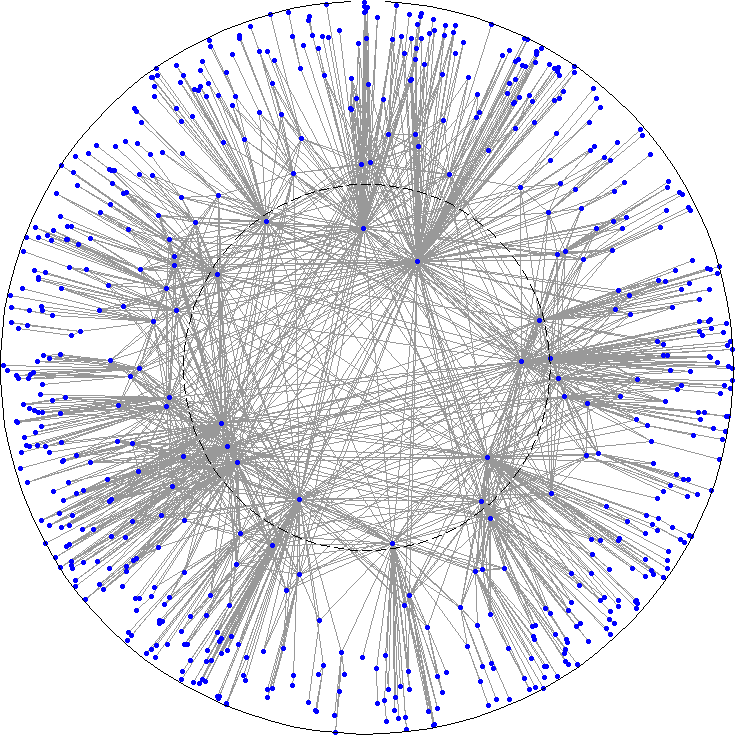
Figure 1: Native representation of the largest connected component (with $621$ vertices) of an instance of $\mathrm{Unf}_{\alpha,C}(n)$ with $\alpha=0.55$, $C=2.25$ and $n=740$. The solid (respectively, segmented) circle is the boundary of $B_{O}(R)$ (respectively, $B_{O}(\frac{R}{2})$).

The adjacency, Laplacian, and normalized Laplacian are three well-known matrices associated to a graph, all of whose spectrum encode important information related to fundamental graph parameters. For non-regular graphs, such as a random hyperbolic graph $G=(V,E)$ obtained from $\mathrm{Unf}_{\alpha,C}(n)$, arguably the most relevant associated matrix is the normalized Laplacian $\mathcal{L}_{G}$. Note that $\mathcal{L}_{G}$ is positive semidefinite and has smallest eigenvalue $0$. Certainly, the most interesting parameter of $\mathcal{L}_{G}$ is its eigenvalue gap $\lambda_{1}(G)$. Since for $\frac{1}{2}<\alpha<1$, a typical occurrence of $G$ has $\Theta(|V|)$ isolated vertices, the eigenvalue $0$ of $G$ has high multiplicity and thus $\lambda_{1}(G)=0$. On the other hand, it is known that for the aforesaid range of $\alpha$, most likely the graph $G$ has a component of linear order [BFM15, Theorem 1.4] (see also Theorem 16 and Corollary 17 below) and all other components are of polylogarithmic order [KM15, Corollary 13], which justifies referring to the linear size component as the giant component. Thus, the most basic non-trivial question about the spectrum of random hyperbolic graphs is to determine the spectral gap of their giant component. Implicit in the proof of [BFM15, Theorem 1.4] (once more, see also Theorem 16 and Corollary 17 below) is that the giant component of a random hyperbolic graph $G$ is the one that contains all vertices whose radial coordinates are at most $\frac{R}{2}$, which we onward refer to as the center component of the hyperbolic graph and denote by $H:=H(G)$.

The preceding discussion motivates our study of the magnitude of the second largest eigenvalue $\lambda_{1}=\lambda_{1}(H)$ of the normalized Laplacian matrix $\mathcal{L}_{H}$ of the center component $H$ of $G$ chosen according to $\mathrm{Unf}_{\alpha,C}(n)$. Formally, denoting by $d(v)$ the degree of $v$ in $G$ (which equals $v$’s degree in $H$), the normalized Laplacian of $H$ is the (square) matrix $\mathcal{L}_{H}$ whose rows and columns are indexed by the vertex set of $H$ and whose $(u,v)$-entry takes the value

$$\mathcal{L}_{H}(u,v):=\begin{cases}1,&\text{if $u=v$},\\ -\displaystyle\frac{1}{\sqrt{d(u)d(v)}},&\text{if $uv$ is an edge of $H$},\\ 0,&\text{otherwise}.\end{cases}$$

Alternatively, $\mathcal{L}_{H}:=I-D_{H}^{-1/2}A_{H}D_{H}^{-1/2}$, where $A_{H}$ denotes the adjacency matrix of $H$ and $D_{H}$ is the diagonal matrix whose $(v,v)$-entry equals $d(v)$. It is well known that $\mathcal{L}_{H}$ is positive semi-definite and its smallest eigenvalue equals $0$ with geometric multiplicity $1$ (given that $H$ is by definition connected). Note that the stochastic matrix associated to the random walk in $H$ is $P_{H}:=D_{H}^{-1}A_{H}=D_{H}^{-1/2}(I-\mathcal{L}_{H})D_{H}^{1/2}$. Hence, results concerning the spectra of $\mathcal{L}_{H}$ easily translate into results about the spectra of $P_{H}$ and thence has implications concerning the rate of convergence towards the stationary distribution of such random walks and related Markov processes.

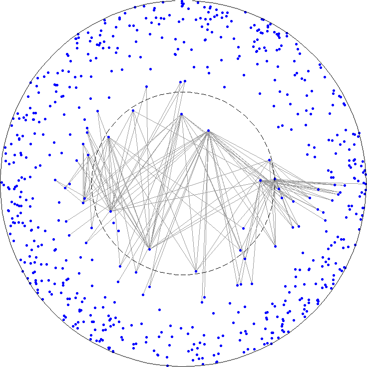
Figure 2: Cut induced in the graph of Figure 1 by vertices of polar coordinate between $0$ and $\pi$ (angles measured relative to a horizontal axis passing through $\mathbb{H}^{2}$’s origin).

One often used approach for bounding $\lambda_{1}(H)$ for a connected graph $H=(U,F)$ is via the so called Cheeger inequality. To explain this, recall that for $S\subseteq U$, the volume of $S$, denoted $\mathrm{vol}(S)$, is defined as the sum of the degrees of the vertices in $S$, i.e., $\mathrm{vol}(S):=\sum_{v\in S}d(v)$. Also, recall that the cut induced by $S$ in $H$, denoted by $\partial S$, is the set of graph edges with exactly one endvertex in $S$, i.e., $\partial S:=\{uv\in F:|\{u,v\}\cap S|=1\}$ (see Figure 2). The conductance of $S$ in $H$, $\emptyset\subsetneq S\subsetneq U$, is defined as

$$h(S):=\frac{|\partial S|}{\min\{\mathrm{vol}(S),\mathrm{vol}(U\setminus S)\}},$$ (2)

and the conductance of $H$ is $h(H):=\min\big{\{}h(S):\emptyset\subsetneq S\subsetneq U\}$. Cheeger’s inequality (see e.g. [Chu97, §2.3]) states that for an arbitrary connected graph $G$,

$$\frac{1}{2}h^{2}(G)\leq\lambda_{1}(G)\leq 2h(G),$$ (3)

and often provides an effective way for bounding the eigenvalue gap of graphs. Our main result gives a stronger characterization of $\lambda_{1}(H)$ than the one obtained through Cheeger’s inequality. In fact, we show that $\lambda_{1}(H)$ essentially matches the upper bound given by (3), i.e., $\lambda_{1}(H)$ equals $h(H)$ up to a small polylogarithmic factor. As a byproduct, we obtain an almost tight bound on the conductance of the giant component of random hyperbolic graphs.

Despite the fact that in the original model of Krioukov et al. [KPK⁺10] $n$ points were chosen uniformly at random, it is from a probabilistic point of view arguably more natural to consider the Poissonized version of this model. Specifically, we consider a Poisson point process on the hyperbolic disk of radius $R$ and denote its point set by $\mathcal{P}$. The intensity function at polar coordinates $(r,\theta)$ for $0\leq r<R$ and $0\leq\theta<2\pi$ is equal to

$$g(r,\theta):=\delta e^{\frac{R}{2}}f(r,\theta)$$

with $\delta=e^{-\frac{C}{2}}$. Throughout the paper we denote this model by $\mathrm{Poi}_{\alpha,C}(n)$. Note in particular that $\int_{0}^{R}\int_{0}^{2\pi}g(r,\theta)d\theta dr=\delta e^{\frac{R}{2}}=n$, and thus $\mathbb{E}|{\mathcal{P}}|=n.$ The main advantage of defining $\mathcal{P}$ as a Poisson point process is motivated by the following two properties: the number of points of $\mathcal{P}$ that lie in any region $A\cap B_{O}(R)$ follows a Poisson distribution with mean given by $\int_{A}g(r,\theta)drd\theta=n\mu(A\cap B_{O}(R))$, and the numbers of points of $\mathcal{P}$ in disjoint regions of the hyperbolic plane are independently distributed. Moreover, by conditioning $\mathcal{P}$ upon the event $|{\mathcal{P}}|=n$, we recover the original distribution. Therefore, since $\mathbf{P}(|{\mathcal{P}}|=n-k)=\Theta(1/\sqrt{n})$ for any $k=O(1)$, any event holding in $\mathcal{P}$ with probability at least $1-o(f_{n})$ must hold in the original setup with probability at least $1-o(f_{n}\sqrt{n})$, and in particular, any event holding with probability at least $1-o(1/\sqrt{n})$ holds a.a.s. in the original model. Also, an event holding w.e.p. in $\mathrm{Poi}_{\alpha,C}(n)$ also holds w.e.p. in $\mathrm{Unf}_{\alpha,C}(n)$. Henceforth, unless stated otherwise, our results will be presented in the Poissonized model only; the corresponding results for the uniform model follow by the above considerations.

Notation. All asymptotic notation in this paper is respect to $n$. Expressions given in terms of other variables such as $O({R})$ are still asymptotics with respect to $n$, since these variables still depend on $n$. We say that an event holds asymptotically almost surely (a.a.s.), if it holds with probability tending to $1$ as $n\to\infty.$ We say that an event holds with extremely high probability (w.e.p.), if for a fixed (but arbitrary) constant $C^{\prime}>0$, there exists an $n_{0}:=n_{0}(C^{\prime})$ such that for every $n\geq n_{0}$ the event holds with probability at least $1-n^{-C^{\prime}}$. Throughout the paper, denote by $\upsilon:=\upsilon(n)$ a function tending to infinity arbitrarily slowly with $n$. By a union bound, we get that the union of polynomially (in $n$) many events that hold w.e.p. is also an event that holds w.e.p. For $N\in\mathbb{N}$, we denote the set $\{1,\ldots,N\}$ by $[N]$. For a graph $G=(V,E)$ with $S,S^{\prime}\subseteq V$ and $S\cap S^{\prime}=\emptyset$, we denote by $E(S,S^{\prime})$ the set of edges having one endvertex in $S$, and one endvertex in $S^{\prime}$. For $v\in V$, we refer to the neighborhood of $v$ inside $S$ by $N_{S}(v)$, i.e., $N_{S}(v)=\{w\in S:vw\in E\}$. Finally, we will often consider a subset $S$ of vertices of a connected component of a given graph in which case $\overline{S}$ will denote its complement with respect to the vertex set of the component.

1.1 Main contributions

The following theorem is the main result of this paper. It bounds from below the spectral gap of random hyperbolic graphs.

Theorem 1.

If $H$ is the center component of $G$ chosen according to $\mathrm{Poi}_{\alpha,C}(n)$ and $D(H)$ denotes the diameter of $H$, then w.e.p.,

$$\lambda_{1}(H)=\Omega(n^{-(2\alpha-1)}/D).$$

We also have the following complementary result. We remark that a similar upper bound, slightly less precise but in the more general setup of geometric inhomogeneous random graphs, was obtained in [BKLa].

Lemma 2.

Let $H=(U,F)$ be the center component of $G=(V,E)$ chosen according to $\mathrm{Poi}_{\alpha,C}(n)$ or $\mathrm{Unf}_{\alpha,C}(n)$. Then, a.a.s. $h(H)\leq\upsilon n^{-(2\alpha-1)}\log n.$

Whereas Theorem 1 gives a global lower bound on the conductance of a random hyperbolic graph, we obtain additional information from the next theorem. By classifying subsets of vertices according to their structure and their volume, we can show the following theorem:

Theorem 3.

Let $H=(U,F)$ be the center component of $G=(V,E)$ chosen according to $\mathrm{Poi}_{\alpha,C}(n)$, and let $0<\varepsilon<1.$ W.e.p., for every set $S\subseteq U$ with $\mathrm{vol}(S)=O(n^{\varepsilon})$, we have $h(S)=\Omega(n^{-(2\alpha-1)\varepsilon+o(1)}).$

We also obtain the following corollary regarding minimum and maximum sizes of arbitrary bisectors (recall that a bisection of a graph is a bipartition of its vertex set in which the number of vertices in the two parts differ by at most $1$, and its size is the number of edges which go across the two parts):

Corollary 4.

Let $H=(U,F)$ be the giant component of $G=(V,E)$ chosen according to $\mathrm{Poi}_{\alpha,C}(n)$. Then, the following statements hold:

• W.e.p., the minimum bisection of $H$ is $b(H)=\Omega\big{(}n^{2(1-\alpha)}/D)$, where $D:=D(H)$ is the diameter of $H$.

• For any $\xi>0$, with probability at least $1-o(n^{-1+\xi})$, the maximum bisection of $H$ is $B(H)=\Theta(n)$.

1.2 Related work

Although the random hyperbolic graph model was relatively recently introduced [KPK⁺10], quite a few papers have analyzed several of its properties. However, none of them deals with the spectral gap of these graphs. In [GPP12], the degree distribution, the maximum degree and global clustering coefficient were determined. The already mentioned paper of [BFM15] characterized the existence of a giant component as a function of $\alpha$; very recently, more precise results including a law of large numbers for the largest component in these networks was established in [FM]. The threshold in terms of $\alpha$ for the connectivity of random hyperbolic graphs was given in [BFMar]. Concerning diameter and graph distances, except for the aforementioned papers of [KM15] and [FK15], the average distance of two points belonging to the giant component was investigated in [ABF]. Results on the global clustering coefficient of the so called binomial model of random hyperbolic graphs were obtained in [CF13], and on the evolution of graphs on more general spaces with negative curvature in [Fou12].

The model of random hyperbolic graphs in the regime where $\frac{1}{2}<\alpha<1$, is very similar to two different models studied in the literature: the model of inhomogeneous long-range percolation in $\mathbb{Z}^{d}$ as defined in [DvdHH13], and the model of geometric inhomogeneous random graphs, as introduced in [BKLb]. In both cases, each vertex is given a weight, and conditionally on the weights, the edges are independent (the presence of edges depending on one or more parameters). In [DvdHH13] the degree distribution, the existence of an infinite component and the graph distance between remote pairs of vertices in the model of inhomogeneous long-range percolation are analyzed. On the other hand, results on typical distances, diameter, clustering coefficient, separators, and existence of a giant component in the model of geometric inhomogeneous graphs were given in [BKLa, BKLb], and bootstrap percolation in the same model was studied in [KL]. Both models are very similar to each other, and similar results were obtained in both cases; since the latter model assumes vertices in a toroidal space, it generalizes random hyperbolic graphs.

1.3 Organization

In Section 2, we give an overview of the general proof strategy. In Section 3, we collect some known general useful results and establish a couple of new ones concerning random hyperbolic graphs that we later rely on. In Section 4, we determine up to polylogarithmic factors both the conductance and the eigenvalue gap of the giant component of random hyperbolic graphs. In Section 5, we essentially show that only linear size vertex sets $S$ of the giant component of random hyperbolic graphs can induce “small bottlenecks” measured in terms of conductance, i.e., if $h(S)$ is approximately equal to the conductance of the giant component $H$, then $S$ must contain essentially a constant fraction of $H$’s vertices. In Section 6, we derive results concerning related graph parameters such as minimum and maximum bisection as well as maximum cuts of random hyperbolic graphs. Finally, in Section 7, we discuss some questions our result naturally raises as well as possible future research directions.

2 Overview of the proof of the main theorems

The proof of Theorem 1 is based on the so called multicommodity flow method. Specifically, it is based on the fact that $\lambda_{1}(H)$ can by its variational characterization be bounded from below as a function of a suitably defined multicommodity flow defined on $H$. Roughly speaking, we aim for finding a flow between all pairs of vertices consisting of not too long paths, and moreover these paths are defined in such a way that no single edge has too much flow going through it. We point out that the classical canonical path technique of routing the flow through one single path cannot give the claimed result, hence we have to split the flow through different edges. Our main task therefore consists in defining such a flow by exploiting properties of the hyperbolic model. In a nutshell, for pairs of vertices “close” to the center we route the flow evenly through paths of length $3$ all of whose vertices are also relatively close to the center. We then extend the flow to pairs of vertices where at least one vertex is “far” from the center by attaching a “shortest” path from each such vertex into the center area; from there on the same strategy of length $3$ paths as before is applied. A crucial ingredient on which the analysis relies concerns properties of the mentioned “shortest” paths implied by the metric of the underlying hyperbolic space. The corresponding upper bound of Lemma 2 is easier, by Cheeger’s inequality it is enough to find an upper bound on the conductance of $H$. The latter can be obtained by considering the set of vertices of $H$ that belong to a half disk of $B_{O}({R})$.

In order to obtain Theorem 3, we decompose the graph in a way that takes into account the underlying geometry. Informally said, the decomposition establishes the existence of regions $\mathcal{R}$ of $B_{O}({R})$ such that for sets of vertices $S$ whose volume is $O(n^{\varepsilon})$ for some $0<\epsilon<1$ the following holds: (i).- $\mathcal{R}$covers a significant fraction of the edges incident to $S$, and (ii).- the fraction of vertices of $\mathcal{R}$ that belong to $S\cap\mathcal{R}$ and to $\overline{S}\cap\mathcal{R}$ are both non-trivial, or both $\mathrm{vol}(S\cap\mathcal{R})$ and $\mathrm{vol}(\overline{S}\cap\mathcal{R})$ are a non-trivial fraction of $\mathrm{vol}(\mathcal{P}\cap\mathcal{R})$. In either case, the number of cut edges of $\partial S$ within $\mathcal{R}$ is relatively large. The main task is to classify sets $S$ according to their shape so that corresponding regions $\mathcal{R}$ can be found.

Additional technical contributions are derived in the process of establishing both theorems. We show that w.e.p. the volume of $H$ is linear in $n$, and that moreover, the volume of a not too small sector is w.e.p. at most proportional to its angle, provided that inside the sector there is no vertex very close to the origin (see Lemma 15 for details). Whereas this result is not surprising, we hope that it will turn out to be useful in other applications as well.

3 Preliminaries

In this section we collect some of the known properties as well as derive some additional ones concerning random hyperbolic graph model. We also state for future reference some known approximations for different terms concerning distances, angles, and measure estimates that are useful in their study.

By the hyperbolic law of cosines (1), the hyperbolic triangle formed by the geodesics between points $p^{\prime}$, $p^{\prime\prime}$, and $p$, with opposing side segments of length $\mathrm{d^{\prime}_{h}}$, $\mathrm{d^{\prime\prime}_{h}}$, and $\mathrm{d_{h}}$ respectively, is such that the angle formed at $p$ is:

$$\theta_{\mathrm{d_{h}}}(\mathrm{d^{\prime}_{h}},\mathrm{d^{\prime\prime}_{h}})=\arccos\Big{(}\frac{\cosh\mathrm{d^{\prime}_{h}}\cosh\mathrm{d^{\prime\prime}_{h}}-\cosh\mathrm{d_{h}}}{\sinh\mathrm{d^{\prime}_{h}}\sinh\mathrm{d^{\prime\prime}_{h}}}\Big{)}.$$ (4)

Clearly, $\theta_{\mathrm{d_{h}}}(\mathrm{d^{\prime}_{h}},\mathrm{d^{\prime\prime}_{h}})=\theta_{\mathrm{d_{h}}}(\mathrm{d^{\prime\prime}_{h}},\mathrm{d^{\prime}_{h}})$. Next, we state a very handy approximation for $\theta_{\mathrm{d_{h}}}(\cdot,\cdot)$.

Lemma 5 ([GPP12, Lemma 3.1]).

If $0\leq\min\{\mathrm{d^{\prime}_{h}},\mathrm{d^{\prime\prime}_{h}}\}\leq\mathrm{d_{h}}\leq\mathrm{d^{\prime}_{h}}+\mathrm{d^{\prime\prime}_{h}}$, then

$$\theta_{\mathrm{d_{h}}}(\mathrm{d^{\prime}_{h}},\mathrm{d^{\prime\prime}_{h}})=2e^{\frac{1}{2}(\mathrm{d_{h}}-\mathrm{d^{\prime}_{h}}-\mathrm{d^{\prime\prime}_{h}})}\big{(}1+\Theta(e^{\mathrm{d_{h}}-\mathrm{d^{\prime}_{h}}-\mathrm{d^{\prime\prime}_{h}}})\big{)}.$$

Remark 6.

We will use the previous lemma also in this form: let $p^{\prime}$ and $p^{\prime\prime}$ be two points at distance $\mathrm{d_{h}}$ from each other such that $r_{p^{\prime}},r_{p^{\prime\prime}}>\frac{R}{2}$ and $\min\{r_{p^{\prime}},r_{p^{\prime\prime}}\}\leq\mathrm{d_{h}}\leq R$. Then, taking $\mathrm{d^{\prime}_{h}}=r_{p^{\prime}}$ and $\mathrm{d^{\prime\prime}_{h}}=r_{p^{\prime\prime}}$ in Lemma 5, we get

$$\theta_{\mathrm{d_{h}}}(r_{p^{\prime}},r_{p^{\prime\prime}}):=2e^{\frac{1}{2}(\mathrm{d_{h}}-r_{p^{\prime}}-r_{p^{\prime\prime}})}\big{(}1+\Theta(e^{\mathrm{d_{h}}-r_{p^{\prime}}-r_{p^{\prime\prime}}})\big{)}.$$

Note also that $\theta_{\mathrm{d_{h}}}(r_{p^{\prime}},r_{p^{\prime\prime}})$, for fixed $r_{p^{\prime}},r_{p^{\prime\prime}}>\frac{R}{2}$, is increasing as a function of $\mathrm{d_{h}}$ (for $\mathrm{d_{h}}$ satisfying the constraints). Below, when aiming for an upper bound, we always use $\mathrm{d_{h}}=R$.

Throughout, we will need estimates for measures of regions of the hyperbolic plane, and more specifically, for regions obtained by performing some set algebra involving a few balls. For a point $p$ of the hyperbolic plane $\mathbb{H}^{2}$, the ball of radius $\rho$ centered at $p$ will be denoted by $B_{p}(\rho)$, i.e., $B_{p}(\rho):=\{q\in\mathbb{H}^{2}:\mathrm{d_{h}}(p,q)\leq\rho\}$.

Also, we denote by $\mu(S)$ the measure of a set $S\subseteq\mathbb{H}^{2}$, i.e.,

$$\mu(S):=\int_{S}f(r,\theta)drd\theta.$$

Next, we collect a few results for such measures.

Lemma 7 ([GPP12, Lemma 3.2]).

If $0\leq\rho<R$, then

$$\mu(B_{O}(\rho))=e^{-\alpha(R-\rho)}(1+o(1)).$$ (5)

Moreover, if $p\in B_{O}(R)$ is such that $r_{p}=r$, then for $C_{\alpha}:=2\alpha/(\pi(\alpha-\frac{1}{2}))$,

$$\mu(B_{p}(R)\cap B_{O}(R))=C_{\alpha}e^{-\frac{r}{2}}\big{(}1+O(e^{-(\alpha-\frac{1}{2})r}+e^{-r})\big{)}.$$ (6)

A direct consequence of (5) is:

Corollary 8.

If $0\leq\rho^{\prime}_{O}<\rho_{O}<R$, then

$$\mu(B_{O}(\rho_{O})\setminus B_{O}(\rho^{\prime}_{O}))=e^{-\alpha(R-\rho_{O})}(1-e^{-\alpha(\rho_{O}-\rho^{\prime}_{O})}+o(1)).$$

Sometimes we will require the following stronger version of (6).

Lemma 9 ([KM15, Lemma 4]).

If $r_{p}\leq\rho_{p}$ and $\rho_{O}+r_{p}\geq\rho_{p}$, then for $C_{\alpha}:=2\alpha/(\pi(\alpha-\frac{1}{2}))$

$$\mu(B_{p}(\rho_{p})\cap B_{O}(\rho_{O}))=C_{\alpha}\big{(}e^{-\alpha(R-\rho_{O})-\frac{1}{2}(\rho_{O}-\rho_{p}+r_{p})}\big{)}+O(e^{-\alpha(R-\rho_{p}+r_{p})}).$$

At several places in this paper we need the following concentration bound.

Theorem 10.

[AS08, Corollary A.1.14] Let $Y$ be the sum of mutually independent indicator random variables, $\mu=\mathbf{E}(Y).$ For all $\epsilon>0$, there is a $c_{\epsilon}>0$ that depends only on $\epsilon$ such that

$$\mathbf{P}(|Y-\mu|>\epsilon\mu)<2e^{-c_{\epsilon}\mu}.$$

For Poisson variables, we also need the following slightly stronger bound:

Theorem 11.

[AS08, Theorem A.1.15] Let $P$ have Poisson distribution with mean $\mu$. For $0<\epsilon<1$,

$$\begin{array}[]{rcl}\mathbf{P}(P\leq\mu(1-\epsilon))&\leq&e^{-\epsilon^{2}\mu/2},\end{array}$$

and for $\epsilon>0$,

$$\begin{array}[]{rcl}\mathbf{P}(P\geq\mu(1+\epsilon))&\leq&\left(e^{-\epsilon}(1+\epsilon)^{-(1+\epsilon))}\right)^{\mu}.\end{array}$$

We immediately derive the following lemma:

Lemma 12.

Let $\mathcal{P}$ be the vertex set of a graph chosen according to $\mathrm{Poi}_{\alpha,C}(n)$. If $S\subseteq B_{O}(R)$ is such that $\mu(S)=\omega(\frac{1}{n}\log n)$, then, w.e.p. $|S\cap\mathcal{P}|=n\mu(S)(1+o(1)).$ Otherwise, w.e.p. $|S\cap\mathcal{P}|\leq\upsilon\log n$.

Many of the proof arguments we will later put forth involve statements concerning sectors of the hyperbolic disk $B_{O}(R)$, in particular, their size and volume. The next two lemmas provide estimates for such quantities. We first provide estimates for the degree of vertices of $G$ as a function of their radius.

Throughout the paper let $\nu^{\prime}:=2\log R+\omega(1)\cap o(\log R)$.

Proposition 13.

Let $v$ be a vertex of $G$ chosen according to $\mathrm{Poi}_{\alpha,C}(n)$. If $r_{v}\leq R-\nu^{\prime}$, then w.e.p. $d(v)=\Theta(e^{\frac{1}{2}(R-r_{v})})$, and if $r_{v}>R-\nu^{\prime}$, then w.e.p. $d(v)\leq(\log n)^{1+o(1)}$.

Proof.

Assume first that $r_{v}\leq R-\nu^{\prime}$. Note that $d(v)=|B_{v}(R)\cap\mathcal{P}|$. Since by Lemma 7 we have $\mu(B_{v}(R)\cap B_{O}(R))=\Theta(e^{-\frac{r_{v}}{2}})=\omega(\frac{\log n}{n})$, by Lemma 12 the first part of the claim follows. If $r_{v}\geq R-\nu^{\prime}$, then $\mu(B_{v}({R})\cap B_{O}({R}))$ is bounded from above by $\mu(B_{w}({R})\cap B_{O}({R}))$ where $w$ is a point of $B_{O}({R})$ with $r_{w}=R-\nu^{\prime}$. We have $\mu(B_{w}({R})\cap B_{O}({R}))=\Theta(e^{\frac{\nu^{\prime}}{2}}/n)=\omega(\frac{\log n}{n})$, and hence by Lemma 12, w.e.p. $d(v)\leq n\mu(B_{w}({R})\cap B_{O}({R}))=O(e^{\frac{\nu^{\prime}}{2}})=(\log n)^{1+o(1)}.$ ∎

When working with a Poisson point process $\mathcal{P}$, for a positive integer $\ell$, we refer to the vertices of $G$ that belong to $B_{O}(\ell)\setminus B_{O}(\ell-1)$ as the $\ell$-th band or layer and denote it by $\mathcal{P}_{\ell}:=\mathcal{P}_{\ell}(G)$, i.e., $\mathcal{P}_{\ell}=\mathcal{P}(G)\cap B_{O}(\ell)\setminus B_{O}(\ell-1)$. We also need estimates for the cardinality and the volume of the $\mathcal{P}_{\ell}$’s.

Since our results are asymptotic, we may and will ignore floors in the following calculations, and assume that certain expressions such as $R-\frac{2\log R}{1-\alpha}$ or the like are integers, if needed. In what follows, also let

$$\ell_{\mathrm{low}} :=\big{\lfloor}(1-\tfrac{1}{2\alpha})R\big{\rfloor},$$

$$\nu :=\tfrac{1}{\alpha}\log R+\omega(1)\cap o(\log R).$$

Proposition 14.

Let $G=(V,E)$ be chosen according to $\mathrm{Poi}_{\alpha,C}(n)$ and let $\mathcal{P}_{\ell}:=\mathcal{P}_{\ell}(G)$.

1. If $\ell\geq\ell_{\mathrm{low}}+\nu$, then w.e.p. $|\mathcal{P}_{\ell}|=\Theta(ne^{-\alpha(R-\ell)})$. Moreover, if $\ell<\ell_{\mathrm{low}}+\nu$, then w.e.p. $|\mathcal{P}_{\ell}|=O(e^{\alpha\nu})=(\log n)^{1+o(1)}$.

2. If $\ell_{\mathrm{low}}+\nu\leq\ell\leq R-\nu^{\prime}$, then w.e.p. $\mathrm{vol}(\mathcal{P}_{\ell})=\Theta(e^{\frac{1}{2}R-(\alpha-\frac{1}{2})(R-\ell)})$.

Proof.

Note that $e^{\alpha\nu}=(\log n)^{1+o(1)}\cap\omega(\log n)$. Consider the first part of the claim. By Lemma 7 we have $\mu(B_{O}(\ell)\setminus B_{O}(\ell-1))=e^{-\alpha(R-\ell)}(1-e^{-\alpha})(1+o(1))$, which is $\omega(\frac{\log n}{n})$ if $\ell\geq\ell_{\mathrm{low}}+\nu$, so the result follows by applying Lemma 12. Assume now that $\ell<\ell_{\mathrm{low}}+\nu$. By Lemma 7 we have that $\mu(B_{O}(\ell_{\mathrm{low}}+\nu))=e^{-\alpha(R-(\ell_{\mathrm{low}}+\nu))}(1+o(1))=\Theta(\frac{e^{\alpha\nu}}{n})=\omega(\frac{\log n}{n})$, so applying again Lemma 12, w.e.p., $|\mathcal{P}_{\ell}|\leq|\mathcal{P}\cap B_{O}(\ell_{\mathrm{low}}+\nu)|=O(e^{\alpha\nu}).$

Since $\mathrm{vol}(\mathcal{P}_{\ell})=\sum_{v\in\mathcal{P}_{\ell}}d(v)$, and for each such vertex $v$, by Proposition 13, its degree is, w.e.p., $\Theta(e^{\frac{1}{2}(R-r_{v})})$, the second part of the claim then follows easily from the first part. ∎

Since the introduction of the random hyperbolic graph model [KPK⁺10], it was pointed out that it gives rise to sparse networks, specifically constant average degree graphs (a fact that was soon after rigorously established in [GPP12]). It follows that the expected volume of random hyperbolic graphs is $\Theta(n)$, and thus their center component has, in expectation, volume $O(n)$. A close inspection of [BFM15] (see Theorem 16 below) actually yields that the volume of the center component is $\Omega(n)$ w.e.p. In this paper, we aim for results that hold w.e.p. and will require very sharp estimates not only for the volume of the center component of random hyperbolic graphs but also for collections of vertices restricted to some regions of $B_{O}(R)$. Next, we describe the regions we will be concerned about. Let $\Phi$ be a $\phi$-sector, that is, $\Phi$ contains all points in $B_{O}(R)$ making an angle of at most $\phi$ at the origin with an arbitrary but fixed reference point. For a vertex $v$, we say that a $\phi$-sector $\Phi$ is centered at $v$ if $v$ lies on the bisector of $\Phi$. Moreover, for a $\phi$-sector $\Phi$ and a vertex $v\in\Phi$, we say that $\Upsilon:=\Phi\setminus B_{O}(r_{v})$ is a sector truncated at $v$, and if in addition $\Phi$ is centered at $v$, then we say it is a sector truncated and centered at $v$. Our next result gives precise estimates for the volume of the center component vertices that belong to sectors and truncated sectors. Although the result is not surprising we believe it is useful to isolate it not only for ease of reference later in this work, but also for reference in follow up work. However, we suggest the reader skip the proof at first reading, due to its rather technical nature.

Lemma 15.

Let $H=(U,F)$ be the center component of $G=(V,E)$ chosen according to $\mathrm{Poi}_{\alpha,C}(n)$. Then, w.e.p. $\mathrm{vol}(U)=O(n)$. Moreover, let $v\in\mathcal{P}_{\ell}$ be such that $\ell\leq(1-\xi)R$ for some arbitrarily small $\xi>0$. If $\Upsilon$ is a sector truncated at $v$ of angle $\phi=\Omega(e^{-\frac{\ell}{2}})$, then w.e.p. $\mathrm{vol}(\Upsilon)=O(\phi n)$.

Proof.

Consider the first part of the lemma. Let $\varepsilon^{\prime}=\varepsilon^{\prime}(\alpha)>0$ be a sufficiently small constant and let $r_{0}=(1-\frac{1}{2\alpha}-\varepsilon^{\prime})R$. By Lemma 7, $\mu(B_{O}(r_{0}))=(1+o(1))e^{-\alpha(R-r_{0})}=\Theta(e^{-(\frac{1}{2}+\alpha\varepsilon^{\prime})R})$. Hence, $|\mathcal{P}\cap B_{O}(r_{0})|$ is a Poisson random variable with mean $t=\Theta(n^{-2\alpha\varepsilon^{\prime}})$. Thus, by Theorem 11, for every $C^{\prime}>0$ there exists a sufficiently large constant $C^{\prime\prime}=C^{\prime\prime}(\alpha)>0$, so that

$$\mathbf{P}\big{(}|\mathcal{P}\cap B_{O}(r_{0})|\geq\tfrac{C^{\prime\prime}}{t}\mathbb{E}(|\mathcal{P}\cap B_{O}(r_{0})|)\big{)}\leq\big{(}\tfrac{3C^{\prime\prime}}{t}\big{)}^{-C^{\prime\prime}}=\Theta(n^{-2\alpha\varepsilon^{\prime}C^{\prime\prime}})\leq n^{-C^{\prime}}.$$

Hence, w.e.p. $|\mathcal{P}\cap B_{O}(r_{0})|\leq C^{\prime\prime}=O(1)$. Thus, by Proposition 13, w.e.p. $\mathrm{vol}(\mathcal{P}\cap B_{O}(r_{0}))=O(n).$ Recall that $\nu=\frac{1}{\alpha}\log R+\omega(1)\cap o(\log R)$. By the same argument, using Corollary 8 and Proposition 13, the total contribution to the volume of vertices $v$ with $r_{0}\leq r_{v}\leq\ell_{\mathrm{low}}+\nu$ is w.e.p.,

$$O\big{(}|\mathcal{P}\cap B_{O}(\ell_{\mathrm{low}}+\nu)|\max_{v\not\in B_{O}(r_{0})}d(v)\big{)}=O(ne^{-\alpha(R-\ell_{\mathrm{low}}-\nu)}e^{\frac{1}{2}(R-r_{0})})=O(n^{\frac{1}{2\alpha}+\varepsilon^{\prime}}e^{\alpha\nu})=o(n),$$

where the last equality follows for sufficiently small $\varepsilon^{\prime}>0$, since $\alpha>\frac{1}{2}$. Similarly, for vertices $v$ with $\ell_{\mathrm{low}}+\nu\leq r_{v}\leq R-\nu^{\prime}$, by Proposition 13 and Proposition 14 part (i), the total volume of these vertices, using the formula for the sum of a geometric series, is w.e.p.,

$$\sum_{\ell=\ell_{\mathrm{low}}+\nu}^{R-\nu^{\prime}}O(ne^{-\alpha(R-\ell)}e^{\frac{1}{2}(R-\ell)})=O(n^{2(1-\alpha)})\sum_{\ell=\ell_{\mathrm{low}}+\nu}^{R-\nu^{\prime}}e^{(\alpha-\frac{1}{2})\ell}=O(ne^{-(\alpha-\frac{1}{2})\nu^{\prime}})=o(n).$$

For the remaining volume, we may at the expense of a factor $2$ assume that all remaining edges are incident to pairs of vertices in $B_{O}(R)\setminus B_{O}(R-\nu^{\prime})$. Fix integers $R-\nu^{\prime}\leq i\leq j\leq R$ and assume $v\in\mathcal{P}_{i}$ and $w\in\mathcal{P}_{j}$. Partition $B_{O}(R)$ into $N:=\lceil\frac{2\pi}{\theta_{R}(i-1,j-1)}\rceil$ sectors denoted (in clockwise order) by $\Phi_{1},\Phi_{2},\ldots,\Phi_{N}$. Observe that if $vw$ is an edge of $G$ then $(v,w)$ besides belonging to $\mathcal{P}_{i}\times\mathcal{P}_{j}$ also belongs to $\Phi_{k}\times\Phi_{k^{\prime}}$ for some $k,k^{\prime}\in[N]$ where $|k-k^{\prime}|\leq 1$. For given $i,j$, let $\mu_{j}^{i}=\frac{1}{N}\mathbb{E}|\mathcal{P}_{j}|$ and $\mu_{i}^{j}=\frac{1}{N}\mathbb{E}|\mathcal{P}_{i}|$. For an integer $c\geq 1$, for either $b=i$ and $a=j$, or $b=j$ and $a=i$, say $\Phi_{k}\cap\mathcal{P}_{b}$ is $c$-regular if $2^{c}\mu_{b}^{a}\leq|\Phi_{k}\cap\mathcal{P}_{b}|\leq 2^{c+1}\mu_{b}^{a}$. Note that $\mu_{b}^{a}=\Theta(n^{2(1-\alpha)}e^{(\alpha-\frac{1}{2})b-\frac{1}{2}a})$ and by Theorem 11, $\Phi_{k}\cap\mathcal{P}_{b}$ is $c$-regular with probability $e^{-\Omega(c2^{c}\mu_{b}^{a})}$. For any ordered pair $(i,j)$ and any $a,b$ as before we have $(\frac{1}{\log n})^{O(1)}\leq\mu_{b}^{a}\leq(\log n)^{O(1)}$. Hence, w.e.p., for every $b$ and every $k$, $|\Phi_{k}\cap\mathcal{P}_{b}|=(\log n)^{O(1)}$.

Let $c,\widetilde{c}\geq 1$ be integers. In expectation, for $i<j$, there are $Ne^{-\Omega(c2^{c}\mu_{i}^{j}+\widetilde{c}2^{\widetilde{c}}\mu_{j}^{i})}$ pairs of sectors $(\Phi_{k},\Phi_{k^{\prime}})$ with $|k-k^{\prime}|\leq 1$ such that $\Phi_{k}\cap\mathcal{P}_{i}$ is $c$-regular and $\Phi_{k^{\prime}}\cap\mathcal{P}_{j}$ is $\widetilde{c}$-regular. Clearly, for a fixed value of $k-k^{\prime}$ $\in\{-1,0,1\}$, disjoint pairs of sectors $(\Phi_{k},\Phi_{k^{\prime}})$ are independent. Hence, if this expectation is $\omega(\log n)$, by Theorem 10, for $i<j$, w.e.p. there are $2Ne^{-\Omega(c2^{c}\mu_{i}^{j}+\widetilde{c}2^{\widetilde{c}}\mu_{j}^{i})}$ such pairs of sectors $(\Phi_{k},\Phi_{k^{\prime}})$, and this also holds after taking a union bound over the three possible values of $k-k^{\prime}$. Otherwise, if the expectation is $O(\log n)$, then w.e.p., by Theorem 10, the number of such pairs is at most $\upsilon\log n$, and since for every $k$ and $b$, we have w.e.p. $|\Phi_{k}\cap\mathcal{P}_{b}|=(\log n)^{O(1)}$, the total number of edges between such pairs of sectors is w.e.p. $(\log n)^{O(1)}$. Similarly, w.e.p., there are $2Ne^{-\Omega(c2^{c}\mu_{i}^{j})}$ pairs of sectors $(\Phi_{k},\Phi_{k^{\prime}})$ with $|k-k^{\prime}|\leq 1$ such that $\Phi_{k}\cap\mathcal{P}_{i}$ is $c$-regular and $|\Phi_{k^{\prime}}\cap\mathcal{P}_{j}|\leq 2\mu_{j}^{i}$ or the expected number of such pairs of sectors is $O(\log n)$, and as before, the number of edges between such pairs of sectors is w.e.p. $(\log n)^{O(1)}$. A similar argument suffices for handling the case of pairs of sectors $(\Phi_{k},\Phi_{k^{\prime}})$ with $|k-k^{\prime}|\leq 1$ such that $|\Phi_{k}\cap\mathcal{P}_{i}|\leq 2\mu_{i}^{j}$ and $\Phi_{k^{\prime}}\cap\mathcal{P}_{j}$ is $\widetilde{c}$-regular. For the remaining pairs of sectors $(\Phi_{k},\Phi_{k^{\prime}})$ we have $|\Phi_{k}\cap\mathcal{P}_{j}|\leq 2\mu_{j}^{i}$ and $|\Phi_{k^{\prime}}\cap\mathcal{P}_{i}|\leq 2\mu_{i}^{j}$. Hence, for the number of edges between $\mathcal{P}_{i}$ and $\mathcal{P}_{j}$, we obtain that w.e.p.,

$$|E(\mathcal{P}_{i},\mathcal{P}_{j})|\leq\sum_{\genfrac{}{}{0.0pt}{}{k,k^{\prime}\in[N]}{|k-k^{\prime}|\leq 1}}|E(\Phi_{k}\cap\mathcal{P}_{i},\Phi_{k^{\prime}}\cap\mathcal{P}_{j})|$$

$$\mbox{}\ =O(N\mu_{i}^{j}\mu_{j}^{i})\big{(}2^{2}\!+\!\!\sum_{c\geq 1}2^{c{+}2}e^{-\Omega(c2^{c}\mu_{i}^{j})}\!+\!\!\sum_{\widetilde{c}\geq 1}2^{\widetilde{c}+2}e^{-\Omega(\widetilde{c}2^{\widetilde{c}}\mu_{j}^{i})}+\!\!\!\!\sum_{c\geq 1,\widetilde{c}\geq 1}\!\!\!2^{c+\widetilde{c}{+}2}e^{-\Omega(c2^{c}\mu_{i}^{j}+\widetilde{c}2^{\widetilde{c}}\mu_{j}^{i})}\big{)}\!+\!(\log n)^{O(1)}$$

$$\mbox{}\ =O\big{(}Nn^{4(1-\alpha)}e^{-(1-\alpha)(i+j)}\big{)}\sum_{c\geq 0}2^{c}e^{-\Omega(c2^{c}\mu_{i}^{j})}\sum_{\widetilde{c}\geq 0}2^{\widetilde{c}}e^{-\Omega(\widetilde{c}2^{\widetilde{c}}\mu_{j}^{i})}+(\log n)^{O(1)}.$$

Now, for $i<j$, observe that since $\alpha<1$, $\mu_{j}^{i}=\Omega(1)$, and hence $\sum_{\widetilde{c}\geq 0}2^{\widetilde{c}}e^{-\Omega(\widetilde{c}2^{\widetilde{c}}\mu_{j}^{i})}=O(1)$. On the other hand, let $c^{*}=c^{*}(i,j):=\min\{c\in\mathbb{N}:2^{c}\mu_{i}^{j}\geq\frac{1}{2}\}.$ Observe that we may ignore values of $c$ smaller than $c^{*}$, as for such pairs of sectors $(\Phi_{k},\Phi_{k^{\prime}})$ no vertices in $\Phi_{k^{\prime}}\cap\mathcal{P}_{i}$ are present, and hence no edges are counted. Then, $\sum_{c\geq c^{*}}2^{c}e^{-\Omega(c2^{c}\mu_{i}^{j})}\leq 2^{c^{*}}\sum_{c^{\prime}\geq 0}2^{c^{\prime}}e^{-\Omega(c^{*}2^{c^{\prime}})}=O\left((2(1-\delta))^{c^{*}}\right)$ for some $\delta>0$. Thus, w.e.p.,

$$|E(\mathcal{P}_{i},\mathcal{P}_{j})|=O\big{(}e^{(\alpha-\frac{1}{2})(i+j)}n^{3-4\alpha})(2(1-\delta))^{c^{*}}+(\log n)^{O(1)}.$$

The same calculations can also be applied for $i=j$ and $k\neq k^{\prime}$. For $i=j$ and $k=k^{\prime}$, edges within the same sector are counted. Hence, since $\mu_{i}^{i}=\Omega(1)$ and thus $\sum_{c\geq 0}2^{2c+2}e^{-\Omega(c2^{c}\mu_{i}^{i})}=O(1)$, we obtain w.e.p. $|E(\mathcal{P}_{i},\mathcal{P}_{i})|=O(e^{(2\alpha-1)i}n^{3-4\alpha})+(\log n)^{O(1)}$. Hence, w.e.p.,

$$\sum_{R-\nu^{\prime}\leq i\leq j\leq R}|E(\mathcal{P}_{i},\mathcal{P}_{j})|=(\log n)^{O(1)}+\sum_{R-\nu^{\prime}\leq i\leq j\leq R}O\big{(}e^{(\alpha-\frac{1}{2})(i+j)}n^{3-4\alpha}(2(1-\delta))^{c^{*}}\big{)}.$$

Now, in order to bound the second right hand side term, write $i=R-\overline{\imath}$, $j=R-\overline{\jmath}$ with $0\leq\overline{\jmath}\leq\overline{\imath}\leq\nu^{\prime}$. Observe that since $2^{c^{*}}=\Theta(1+n^{-2(1-\alpha)}e^{\frac{1}{2}j-(\alpha-\frac{1}{2})i)})=\Theta(1+e^{(\alpha-\frac{1}{2})\overline{\imath}-\frac{1}{2}\overline{\jmath}})$. Consider first pairs $(i,j)$ with $c^{*}=O(1)$. For such pairs,

$$n^{3-4\alpha}\sum_{R-\nu^{\prime}\leq i\leq j\leq R}e^{(\alpha-\frac{1}{2})(i+j)}=O(n)\sum_{0\leq\overline{\jmath}\leq\overline{\imath}\leq\nu^{\prime}}e^{(\alpha-\frac{1}{2})(-\overline{\imath}-\overline{\jmath})}=O(n),$$

where we used the formula for a geometric series. Consider then pairs $(i,j)$ with $c^{*}=\omega(1)$. For such a pair, $2^{c^{*}}=\Theta(e^{(\alpha-\frac{1}{2})\overline{\imath}-\frac{1}{2}\overline{\jmath}})$, we have $(2(1-\delta))^{c^{*}}=\Theta(e^{(1-\delta^{\prime})\left((\alpha-\frac{1}{2})\overline{\imath}-\frac{1}{2}\overline{\jmath}\right)})$ for some $0<\delta^{\prime}<1$. Hence,

$$n^{3-4\alpha}\sum_{R-\nu^{\prime}\leq i\leq j\leq R}O\big{(}(2(1-\delta))^{c^{*}}e^{(\alpha-\frac{1}{2})(i+j)}\big{)}=O(n)\sum_{0\leq\overline{\jmath}\leq\overline{\imath}\leq\nu^{\prime}}e^{-\alpha\overline{\jmath}}e^{-\delta^{\prime}((\alpha-\frac{1}{2})\overline{\imath}-\frac{1}{2}\overline{\jmath})}$$

$$=O(n)\sum_{0\leq\overline{\imath}\leq\nu^{\prime}}e^{-\delta^{\prime}(\alpha-\frac{1}{2})\overline{\imath}}\sum_{\overline{\jmath}=0}^{\overline{\imath}}e^{(-\alpha+\frac{\delta^{\prime}}{2})\overline{\jmath}}=O(n)\sum_{0\leq\overline{\imath}\leq\nu^{\prime}}e^{-\delta^{\prime}(\alpha-\frac{1}{2})\overline{\imath}}=O(n),$$

where we again used the formula for a geometric series, thus finishing the proof of the first part of the claimed result.

Now, consider the second part of the lemma, and let $v\in\mathcal{P}_{\ell}$ with $\ell=\lambda R\leq(1-\xi)R$ for some arbitrarily small $\xi>0$. Since $\phi=\Omega(n^{-\lambda})$, we may partition $\Upsilon$ into $t=\Theta(\frac{\phi}{n^{-\lambda}})$ subsectors $T_{1},\ldots,T_{t}$ of angle $\Theta(n^{-\lambda})$ and bound the volume of each subsector $T_{k}$ separately. Let $\widehat{\lambda}$ be such that $1-\lambda-2\alpha(1-\widehat{\lambda})=-\varepsilon^{\prime}$ for sufficiently small $\varepsilon^{\prime}=\varepsilon^{\prime}(\alpha)>0$. Note that since $\alpha>\frac{1}{2}$, for $\varepsilon^{\prime}$ small enough, we have $1>\widehat{\lambda}>\lambda$. For a fixed $T_{k}$, consider first vertices $w\in\mathcal{P}\cap T_{k}$ with $\ell\leq r_{w}\leq\widehat{\ell}:=\lfloor\widehat{\lambda}R\rfloor$. Since the expected number of vertices of such radius inside $T_{k}$, by Lemma 7 and the choice of angle for defining $T_{k}$, is $O(n^{-\varepsilon^{\prime}})$, by the same reasoning as in the first part of the lemma, w.e.p. there are $O(1)$ such vertices, and their total volume is, by Proposition 13, w.e.p. $O(1)e^{\frac{1}{2}(R-\ell)}=O(n^{1-\lambda})$. Next, let $\overline{\lambda}$ be such that $1-\lambda-2\alpha(1-\overline{\lambda})=\varepsilon^{\prime}$. Note that $1>\overline{\lambda}>\widehat{\lambda}$ and consider vertices $w\in\mathcal{P}\cap T_{k}$ with $\widehat{\ell}\leq r_{w}\leq\overline{\ell}:=\lfloor\overline{\lambda}R\rfloor$. As in the first part of the lemma, the total contribution of these vertices to the volume of $T_{k}$ is, w.e.p.,

$$O(e^{\frac{1}{2}(R-\widehat{\ell})}n^{1-\lambda}e^{-\alpha(R-\overline{\ell})})=O(n^{1-\widehat{\lambda}+\varepsilon^{\prime}})=O(n^{\frac{1-\lambda+\epsilon^{\prime}}{2\alpha}+\varepsilon^{\prime}})=o(n^{1-\lambda}),$$

where the last equality follows by choosing $\varepsilon^{\prime}=\varepsilon^{\prime}(\alpha)$ sufficiently small.

Next, let us consider vertices $w\in\mathcal{P}\cap T_{k}$ with $\overline{\ell}\leq r_{w}\leq R-\nu^{\prime}$. By the same argument as in the first part of the lemma, the total volume of such vertices is w.e.p.,

$$\sum_{\ell^{\prime}=\overline{\ell}}^{R-\nu^{\prime}}O(n^{1-\lambda}e^{-\alpha(R-\ell^{\prime})})e^{\frac{1}{2}(R-\ell^{\prime})}=o(n^{1-\lambda}).$$

As before, we may assume that the remaining edges are incident to pairs of vertices in $B_{O}(R)\setminus B_{O}(R-\nu^{\prime})$, with at least one vertex inside $T_{k}$. Since most vertices indeed have all its neighbors inside $T_{k}$, we may in fact also consider only pairs of vertices in $T_{k}\setminus B_{O}(R-\nu^{\prime})$. For these pairs, the argument is as before, we fix integers $R-\nu^{\prime}\leq i\leq j\leq R$, and partition $T_{k}$ into $\lceil\frac{\phi}{\theta_{R}(i-1,j-1)}\rceil$ sectors of equal angle. Since $\lambda<1$, the same argument as in the first part, replacing the number of sectors $N$ by $O(Nn^{-\lambda})$, shows that the number of such edges is w.e.p. $O(n^{1-\lambda})$. Hence, since $\mathrm{vol}(\Upsilon)=\sum_{k}\mathrm{vol}(T_{k})$, and for each $k$, w.e.p. $\mathrm{vol}(T_{k})=O(n^{1-\lambda})$, we have w.e.p. $\mathrm{vol}(\Upsilon)=O(tn^{1-\lambda})=O(\phi n)$, and the second part of the lemma is finished as well. ∎

Recall that a $\pi$-sector is a $\phi$-sector with angle $\pi$, that is a half disk. Next, we combine our previous lemma with known facts about the giant component of random hyperbolic graphs in order to observe that both the volume and the size of their center component are linear in $n$, and that this holds even if one considers only the vertices that belong to a fixed $\pi$-sector of $B_{O}(R)$.

Theorem 16.

[Theorem 1.4 of [BFM15]] Let $H=(U,F)$ be the center component of $G=(V,E)$ chosen according to $\mathrm{Poi}_{\alpha,C}(n)$. Let $\Pi$ is a $\pi$-sector, then w.e.p. $|U\cap\Pi|=\Omega(n)$. Moreover, w.e.p. $H$ is the giant component of $G$.

Proof.

A close inspection of Theorem 1.4 part (ii) of [BFM15] shows that it can also be performed in the model $\mathrm{Poi}_{\alpha,C}(n)$. Moreover, after suitably adapting the value of $C$ and thus of $T$ as defined in Section 4.2 of [BFM15], equation (4.21) and then also Lemma 4.2 of [BFM15] in fact hold w.e.p., and thus, the proof given there shows that w.e.p. $|U|=\Omega(n)$. The same proof holds also when restricting to one half of $B_{O}(R)$, and hence w.e.p. $|U\cap\Pi|=\Omega(n)$. For the second part of the corollary, once more a close inspection of the same theorem (Lemma 4.1, equations (4.3) and (4.21) of Theorem 1.4 of  [BFM15]) show that the claimed result holds in the Poisson model, and it holds w.e.p. ∎

An immediate consequence of Lemma 15 and Theorem 16 is the following:

Corollary 17.

Let $H=(U,F)$ be the center component of $G=(V,E)$ chosen according to $\mathrm{Poi}_{\alpha,C}(n)$. Then, w.e.p. $\mathrm{vol}(U)=\Theta(n)$. Moreover, if $\Pi$ is a $\pi$-sector, then w.e.p. $\mathrm{vol}(U\cap\Pi)\geq|U\cap\Pi|=\Omega(n)$.

Regarding the diameter of the center component, we have the following result:

Theorem 18.

[Theorem 1 and Theorem 3 of [FK15]] Let $H=(U,F)$ be the center component of $G=(V,E)$ chosen according to $\mathrm{Poi}_{\alpha,C}(n)$ and let $D=D(H)$ denote its diameter. Then, w.e.p.,

$$D=\Omega(\log n)\cap O((\log n)^{\frac{1}{1-\alpha}}).$$

Proof.

Again, the results stated in [FK15] are stated with smaller probability, but a close inspection of them shows that they hold w.e.p. The original results are stated in the uniform model, but again, they hold in the Poissonized model as well. ∎

The following lemma is implicit in [BFM15], we make it explicit here.

Lemma 19.

Let $H=(U,F)$ be the center component of $G=(V,E)$ chosen according to $\mathrm{Poi}_{\alpha,C}(n)$. If $\Phi$ is a $\phi$-sector with $\phi=\omega(\frac{1}{n}(\log n)^{\frac{1+\alpha}{1-\alpha}})$, then, w.e.p. $\mathrm{vol}(U\cap\Phi)\geq|U\cap\Phi|=\Omega(\phi n(\log n)^{-\frac{2\alpha}{1-\alpha}})$.

Proof.

Let $\ell_{\mathrm{bdr}}:=\lfloor R-\frac{2\log R}{1-\alpha}\rfloor$. Since $d(v)\geq 1$ for any $v\in U$, the inequality $\mathrm{vol}(U\cap\Phi)\geq|U\cap\Phi|$ is trivial. In order to show that $|U\cap\Phi|=\Omega(\phi n(\log n)^{\frac{2\alpha}{1-\alpha}})$, note that, using the lower bound on $\phi$, by Lemma 7 and Lemma 12, the number of vertices in $\Phi\cap\mathcal{P}_{\ell_{\mathrm{bdr}}}$ is w.e.p. $\Theta(\phi n(\log n)^{-\frac{2\alpha}{1-\alpha}})$. Note also that for every vertex $v\in\mathcal{P}_{\ell}$ with $\frac{R}{2}\leq\ell\leq\ell_{\mathrm{bdr}}$, by Remark 6 and Corollary 8, the expected number of neighbors of $v$ inside $\mathcal{P}_{\ell-1}$ is $\Theta(ne^{-\alpha(R-\ell)}e^{\frac{1}{2}(R-2\ell)})=\Omega(\log^{2}n)$, and hence, by Lemma 12 this holds w.e.p. Thus, all vertices $v\in\mathcal{P}_{\ell}$ connect through consecutive layers to vertices that belong to $B_{O}(\frac{R}{2})$ and thus are part of the center component $H$. Hence, $|U\cap\Phi|=\Omega(\phi n(\log n)^{-\frac{2\alpha}{1-\alpha}})$. ∎

To conclude this section, we make a final important observation that simplifies arguing about the center component (and thus the giant component) of random hyperbolic graphs.

Remark 20.

The previous lemma shows that w.e.p. all vertices in $\mathcal{P}\cap B_{O}(R-\frac{2\log R}{1-\alpha})$ in fact belong to the center component, and hence, for each $\ell\leq R-\frac{2\log R}{1-\alpha}$, w.e.p. $\mathcal{P}_{\ell}(G)=\mathcal{P}_{\ell}(H).$ We will use this without further mention throughout the paper.

4 Spectral gap

The purpose of this section is to bound from below the spectral gap of the center component $H$ of a random hyperbolic graph, i.e., proving Theorem 1. As we show next, this result is essentially tight. Indeed, we first prove Lemma 2 by showing a simple upper bound for $\lambda_{1}(H)$ obtained via Cheeger’s inequality, that is, via an upper bound on the graph conductance of $H$. We include the bound mainly for completeness sake.

Proof of Lemma 2. Let $\Pi$ be a $\pi$-sector. We have to show that $h(\Pi)\leq\upsilon n^{-(2\alpha-1)}\log n$. Let $\mathcal{P}$ be the set of vertices (points) if $G$ is chosen according to $\mathrm{Poi}_{\alpha,C}(n)$, and let $\mathcal{U}$ be the set of vertices (points) if $G$ is chosen according to $\mathrm{Unf}_{\alpha,C}(n)$. First, observe that by Corollary 17 w.e.p. $\mathrm{vol}(\Pi)=\Theta(n)$, $\mathrm{vol}(\mathcal{P}\setminus\Pi)=\Theta(n)$. Since Corollary 17 holds w.e.p., the same results clearly hold in the uniform model as well. Hence, it suffices to show that a.a.s. $|E(\Pi,\mathcal{U}\setminus\Pi)|,|E(\Pi,\mathcal{P}\setminus\Pi)|=n^{2(1-\alpha)}O(\log n)$. Define $\mathcal{U}_{N}$ as a uniformly distributed set of $N$ points in the hyperbolic disk of radius $R=2\log n+C$, i.e., $\mathcal{U}_{N}$ equals $\mathcal{P}$ conditioned on $|\mathcal{P}|=N$. We first determine the expected value of $|E(\Pi,\mathcal{U}_{N}\setminus\Pi)|$. Clearly,

$$\mathbf{E}(|E(\Pi,\mathcal{U}_{N}\setminus\Pi)|)=2\binom{N}{2}\mathbf{P}(u\in\Pi,v\in\mathcal{U}_{N}\setminus\Pi,\mathrm{d_{h}}(r_{u},r_{v},\theta_{u}-\theta_{v})\leq R).$$

We divide the computation of the latter probability into two cases depending on whether or not $r_{u}+r_{v}\leq R$, and denote the corresponding probabilities by $P^{\prime}$ and $P^{\prime\prime}$. Recalling that $C(\alpha,R)=\cosh(\alpha R)-1$ and since $2\sinh x\sinh y=\cosh(x+y)-\cosh(x-y)$,

$$P^{\prime} =\frac{1}{4}\iint_{r_{u}+r_{v}\leq R}f(r_{u})f(r_{v})dr_{v}dr_{u}=\frac{\alpha^{2}}{4(C(\alpha,R))^{2}}\iint_{r_{u}+r_{v}\leq R}\sinh(\alpha r_{u})\sinh(\alpha r_{v})dr_{v}dr_{u}$$

$$=\frac{\alpha}{8(C(\alpha,R))^{2}}R\sinh(\alpha R)-\frac{1}{4C(\alpha,R)}=O(R)e^{-\alpha R}=n^{-2\alpha}O(\log n).$$

Now, in order to compute $P^{\prime\prime}$, observe that if for $u\in\Pi$, $v\in\mathcal{U}_{N}\setminus\Pi$ with $r_{u}+r_{v}\geq R$, we have $uv\in F$, then either $\theta_{u}+(2\pi-\theta_{v})\leq\theta_{R}(r_{u},r_{v})$ or $\theta_{v}-\theta_{u}\leq\theta_{R}(r_{u},r_{v})$, where $\theta_{R}(\cdot,\cdot)$ is as defined in (4). Clearly, for $(\theta_{u},\theta_{v})\in[0,\pi)\times[\pi,2\pi)$ the area of both triangles defined by the aforestated two inequalities is $\theta_{R}(r_{u},r_{v})$, and hence the probability that $(\theta_{u},\theta_{v})$ satisfies one of the two inequalities is $\frac{1}{4\pi^{2}}\theta^{2}_{R}(r_{u},r_{v})$. Thus, by Lemma 5,

$$P^{\prime\prime} =\frac{1}{4\pi^{2}}\iint_{r_{u}+r_{v}\geq R}\theta^{2}_{R}(r_{u},r_{v})f(r_{u})f(r_{v})dr_{u}dr_{v}$$

$$=\frac{\alpha^{2}}{\pi^{2}(C(\alpha,R))^{2}}\iint_{r_{u}+r_{v}\geq R}e^{R-r_{u}-r_{v}}(1+\Theta(e^{R-r_{u}-r_{v}}))\sinh(\alpha r_{u})\sinh(\alpha r_{v})dr_{u}dr_{v}$$

$$=\frac{\alpha^{2}e^{R}}{4\pi^{2}(C(\alpha,R))^{2}}\iint_{r_{u}+r_{v}\geq R}e^{-(1-\alpha)(r_{u}+r_{v})}(1+O(e^{R-r_{u}-r_{v}}+e^{-2\alpha r_{u}}+e^{-2\alpha r_{v}}))dr_{u}dr_{v}$$

$$=O(R)e^{-\alpha R}=n^{-2\alpha}O(\log n).$$

Summarizing, for $N=n$ and the model $\mathrm{Unf}_{\alpha,C}(n)$, we have $\mathbf{E}(|E(\Pi,\mathcal{U}\setminus\Pi)|)=O(n^{2(1-\alpha)}\log n)$. For the model $\mathrm{Poi}_{\alpha,C}(n)$,

$$\mathbf{E}(|E(\Pi,\mathcal{P}\setminus\Pi)|) =\sum_{N\geq 0}\mathbf{E}(|E(\Pi,\mathcal{U}_{N}\setminus\Pi)|)\mathbf{P}(|\mathcal{P}|=N)=O(n^{-2\alpha}\log n)\sum_{N\geq 0}\binom{N}{2}e^{-n}\frac{n^{N}}{N!}$$

$$=O(n^{2(1-\alpha)}\log n)\sum_{N\geq 2}e^{-n}\frac{n^{N-2}}{(N-2)!}=O(n^{2(1-\alpha)}\log n).$$

In either case, the desired statement follows by Markov’s inequality. ∎

We now undertake the more challenging task of establishing a lower bound on the spectral gap of the center component of random hyperbolic graphs. By Theorem 18, w.e.p. the diameter of the giant component of a graph chosen according to $\mathrm{Unf}_{\alpha,C}(n)$ is $O((\log n)^{\frac{1}{1-\alpha}})$ when $\frac{1}{2}<\alpha<1$. A well known relation between the spectral gap and the diameter of graphs (see for example [Chu97, Lemma 1.9]) establishes that for a connected graph $G$ with diameter $D$ it holds that $\lambda_{1}(G)\geq 1/(D\mathrm{vol}(V(G)))$. Thus, since by Corollary 17, w.e.p. $\mathrm{vol}(V(H))=\Theta(n)$, we get that $\lambda_{1}(H)=\Omega(\frac{1}{n}(\log n)^{-\frac{1}{1-\alpha}})$. Since by Lemma 2 we have $h(H)\leq\upsilon n^{-(2\alpha-1)}\log n$, the lower bound on $\lambda_{1}(H)\geq\frac{1}{2}h^{2}(H)$ obtained from Cheeger’s inequality (see (3)) cannot be asymptotically tight when $\alpha>\frac{3}{4}$. Below, we prove a lower bound on $\lambda_{1}(H)$ which in fact establishes that up to polylogarithmic (in $n$) factors, the upper bound given by Cheeger’s inequality is asymptotically tight.

In order to bound $\lambda_{1}(H)$ from below we rely on the multicommodity flow technique developed in [DS91, Sin92]. The basic idea is to consider a multicommodity flow problem in the graph and obtain lower bounds on $\lambda_{1}(H)$ in terms of a measure of flows. Formally, a flow in $H$ is a function $f$ mapping a collection of (oriented) simple paths $\mathcal{Q}:=\mathcal{Q}(H)$ in $H=(U,F)$ to the positive reals which satisfies, for all $s,t\in U$, $s\neq t$, the following flow demand constraint:

$$\sum_{q\in\mathcal{Q}_{s,t}}f(q)=\frac{d(s)d(t)}{\mathrm{vol}(U)},$$ (7)

where $\mathcal{Q}_{s,t}$ is the set of all (oriented) paths $q\in\mathcal{Q}$ from $s$ to $t$. Clearly, an extension of $f$ to a function on oriented edges of $H$ is obtained by setting $f(e)$ equal to the total flow routed by $f$ through the oriented edge $e$, i.e., $f(e):=\sum_{q\ni e}f(q)$.

In order to measure the quality of the flow $f$ a function on oriented edges, denoted $\overline{f}$, is defined by

$$\overline{f}(e):=\sum_{q\in\mathcal{Q}:q\ni e}f(q)|q|,$$ (8)

where $|q|$ is the length (number of edges) of the path $q$. The term $\overline{f}(e)$ is referred to as the elongated flow through $e$. The flow’s quality is captured by the quantity $\overline{\rho}(f):=\max_{e}\overline{f}(e)$, where the maximum is taken over oriented edges. The following result is the cornerstone of the multicommodity flow method. We include the claim’s proof for several reasons; (i)- for concreteness sake, (ii)- due to its elegance and conciseness, and (iii)- for clarity of exposition, because in all instances known to us, the result is stated in the language of reversible Markov chains, and its interpretation in graph theoretic terms might not be straightforward for the reader.

Theorem 21 (Sinclair [Sin92]).

If $f$ is a flow in a connected graph $H=(U,F)$, then

$$\lambda_{1}(H)\geq\frac{1}{\overline{\rho}(f)}.$$

Proof.

Recall (see e.g. [Chu97, Eqn. (1.5)]) the following characterization of

$$\lambda_{1}:=\lambda_{1}(H)=\inf_{\psi}\frac{\sum_{s,t:st\in F}(\psi(s)-\psi(t))^{2}}{\sum_{s,t\in U}(\psi(s)-\psi(t))^{2}\frac{d(s)d(t)}{\mathrm{vol}(U)}},$$

where the infimum is taken over all non-constant functions $\psi:U\to\mathbb{R}$.

For an oriented edge $e$, let $e^{-}$ and $e^{+}$ denote its start- and endvertices. Note now that for any $\psi$ and any flow $f$ in $H$, the denominator of the last displayed equation can be bounded from above as follows:

$$\sum_{s,t\in U}(\psi(s)-\psi(t))^{2}\frac{d(s)d(t)}{\mathrm{vol}(U)}=\sum_{s,t\in U}\sum_{q\in\mathcal{Q}_{s,t}}f(q)\big{(}\sum_{e\in q}(\psi(e^{-})-\psi(e^{+}))\big{)}^{2}$$

$$\mbox{}\qquad\leq\sum_{q\in\mathcal{Q}}f(q)|q|\sum_{e\in q}(\psi(e^{-})-\psi(e^{+}))^{2}=\sum_{e}(\psi(e^{-})-\psi(e^{+}))^{2}\overline{f}(e)$$

$$\mbox{}\qquad\leq\overline{\rho}(f)\sum_{e}(\psi(e^{-})-\psi(e^{+}))^{2}=\overline{\rho}(f)\sum_{s,t:st\in F}(\psi(s)-\psi(t))^{2},$$

where the first inequality is by Cauchy-Schwarz, and the second one by definition of $\overline{\rho}(f)$. (Note that the first equality in the preceding displayed derivation requires that $\mathcal{Q}_{s,t}$ is non-empty for all $s,t\in U$, which is indeed the case given that $H$ is connected.) ∎

A particular version of the multicommodity flow method, referred to as the canonical path method, consists in routing, for every pair of distinct vertices $s,t\in U$, the required $d(s)d(t)/\mathrm{vol}(U)$ flow demand via a single oriented path going from $s$ to $t$. This simplified method cannot deliver as strong bounds on $\lambda_{1}(H)$ as the ones we claim. Indeed, for the canonical path method, the elongated flow on any edge used by a path carrying flow from $s$ to $t$ must be at least $d(s)d(t)/\mathrm{vol}(U)$. Taking $s$ and $t$ as the maximum degree vertices in $H$, known results on the maximum degree of hyperbolic random graphs (see [GPP12, Theorem 2.4]) lead to bounds on elongated flows not smaller than $\Omega(n^{\frac{1}{\alpha}-1})$, and thence to bounds on $\lambda_{1}(H)$ no better than $O(n^{1-\frac{1}{\alpha}})$, which would be worse than the claimed lower bound of $\Omega(n^{-(2\alpha-1)}/D)$ if $\alpha<\frac{1}{\sqrt{2}}$ (with some effort maybe one might be able to show that the method does not provide strong bounds even for larger values of $\alpha$).

To simplify the exposition, we will use Theorem 21 in a slightly easily derived variant stated below. First, say that $\{\mathcal{Q}^{\prime},\mathcal{Q}^{\prime\prime}\}$ is a path consistent partition of $\mathcal{Q}:=\mathcal{Q}(H)$ provided there is a path oriented from $s$ to $t$ in $\mathcal{Q}^{\prime}$ if and only if no such path is found in $\mathcal{Q}^{\prime\prime}$, i.e., for all $s,t\in U$, $s\neq t$, the set $\mathcal{Q}^{\prime}_{s,t}$ is non-empty if and only if $\mathcal{Q}^{\prime\prime}_{s,t}$ is empty. Moreover, for $\widetilde{\mathcal{Q}}\subseteq\mathcal{Q}$, we say $\widetilde{f}:\mathcal{Q}\to\mathbb{R}_{+}$ is a $\widetilde{\mathcal{Q}}$-flow provided $\widetilde{f}(q)=0$ if $q\not\in\widetilde{\mathcal{Q}}$ and for every $s,t\in U$, $s\neq t$ such that $\widetilde{\mathcal{Q}}_{s,t}$ is non-empty, the following holds:

$$\sum_{q\in\widetilde{Q}_{s,t}}\widetilde{f}(q)=\frac{d(s)d(t)}{\mathrm{vol}(U)}.$$ (9)

We extend to $\widetilde{Q}$-flows, in the natural way, the notions of elongated flow and maximum elongated flow. In order to more easily apply Theorem 21 we will construct a flow satisfying its hypothesis as a sum of $\widetilde{Q}$-flows. Our next result validates such an approach.

Corollary 22.

Let $H=(U,F)$ be a connected graph and $\{\mathcal{Q}^{\prime},\mathcal{Q}^{\prime\prime}\}$ a path consistent partition of $\mathcal{Q}:=\mathcal{Q}(H)$. Let $f^{\prime},f^{\prime\prime}:\mathcal{Q}\to\mathbb{R}_{+}$ be such that $f^{\prime}$ is a $\mathcal{Q}^{\prime}$-flow and $f^{\prime\prime}$ is a $\mathcal{Q}^{\prime\prime}$-flow, then $f^{\prime}+f^{\prime\prime}$ is a flow in $H$ and

$$\overline{\rho}(f^{\prime}+f^{\prime\prime})\leq\overline{\rho}(f^{\prime})+\overline{\rho}(f^{\prime\prime}).$$

Proof.

The result follows since $\overline{\rho}(f^{\prime}+f^{\prime\prime})=\max_{e}\big{(}\overline{f^{\prime}}(e)+\overline{f^{\prime\prime}}(e)\big{)}\leq\overline{\rho}(f^{\prime})+\overline{\rho}(f^{\prime\prime})$. ∎

Key to our approach is the fact that w.e.p. random hyperbolic graphs admit multicommodity flows of moderate maximum elongated flow. To prove this assertion we associate to the center component $H$ of $G$ chosen according to $\mathrm{Poi}_{\alpha,C}(n)$ a path consistent partition $\{\mathcal{Q}^{\prime},\mathcal{Q}^{\prime\prime}\}$ of $\mathcal{Q}:=\mathcal{Q}(H)$. The collection $\mathcal{Q}^{\prime}$ will consist of paths whose endvertices are both “sufficiently close” to the origin $O$. In contrast, $\mathcal{Q}^{\prime\prime}$ will consist of the collection of paths one of whose endvertices is not “sufficiently close” to the origin $O$. We will fix the flow for path $q$ with endvertices $s$ and $t$, so that it satisfies (7) while distributing an equal amount of flow among all paths in $\mathcal{Q}_{s,t}$.

In addition to the already defined quantities $\ell_{\mathrm{low}}=\lfloor(1-\frac{1}{2\alpha})R\rfloor$ and $\nu^{\prime}=2\log R+\omega(1)\cap o(\log R)$, the following quantities will also play an important role in the construction of $\mathcal{Q}^{\prime}$ and $\mathcal{Q}^{\prime\prime}$:

$$\ell_{\mathrm{min}} :=\big{\lceil}(\alpha-\tfrac{1}{2})R+\nu^{\prime}\big{\rceil},$$ (10)

$$\ell_{\mathrm{mid}} :=\big{\lfloor}\tfrac{R}{2}\big{\rfloor},$$ (11)

$$\ell_{\mathrm{max}} :=\big{\lfloor}(\tfrac{3}{2}-\alpha)R-\nu^{\prime}\big{\rfloor}.$$ (12)

Observe that $\ell_{\mathrm{min}}+\ell_{\mathrm{max}}=R$. For sufficiently large $n$, it always holds that $\ell_{\mathrm{min}}<\ell_{\mathrm{mid}}<\ell_{\mathrm{max}}$ and $\ell_{\mathrm{min}}<\ell_{\mathrm{low}}+\nu<\ell_{\mathrm{mid}}$. From now on, we assume without further mention that $n$ is large enough so that these inequalities hold. Henceforth, for an integer $\ell\leq\ell_{\mathrm{max}}$, we let

$$\widetilde{\ell}=\begin{cases}\ell_{\mathrm{max}},&\text{if $\ell<\ell_{\mathrm{min}}$,}\\ 2\ell_{\mathrm{mid}}-\ell+1,&\text{if $\ell_{\mathrm{min}}\leq\ell\leq\ell_{\mathrm{mid}}$,}\\ \ell_{\mathrm{mid}},&\text{if $\ell>\ell_{\mathrm{mid}}$}.\end{cases}$$

Note that $\frac{R}{2}\geq\ell_{\mathrm{mid}}=\frac{R}{2}+\Theta(1)$ and $\ell_{\mathrm{mid}}\leq\widetilde{\ell}\leq\ell_{\mathrm{max}}$. Moreover, observe that $\ell\leq\ell_{\mathrm{mid}}$ if and only if $\widetilde{\ell}>\ell_{\mathrm{mid}}$. As before, often we shall ignore the floors/ceilings in the preceding definitions, since it only introduces low order term approximations in our derivations. Recall that whenever referring to expressions such as $R-\frac{\log R}{1-\alpha}$ or the like, when needed, we will also assume that these are integers.

Details concerning $\mathcal{Q}^{\prime}$ as well as an associated $\mathcal{Q}^{\prime}$-flow are provided in the next section, and in the subsequent one analogous results concerning $\mathcal{Q}^{\prime\prime}$ are discussed.

4.1 A $\mathcal{Q}^{\prime}$-flow

For $s\in\mathcal{P}_{k}$ and $t\in\mathcal{P}_{k^{\prime}}$ with $k,k^{\prime}\leq\ell_{\mathrm{max}}$, let ${\mathcal{Q}^{\prime}}_{s,t}$ be the collection of length $3$ oriented paths from $s$ to $t$ whose first internal vertex belongs to $\mathcal{P}_{\widetilde{k}}$ and the other internal vertex is in $\mathcal{P}_{\widetilde{k^{\prime}}}$. Also, let ${\mathcal{Q}^{\prime}}$ be the union of all such $\mathcal{Q}^{\prime}_{s,t}$’s. We classify paths in $\mathcal{Q}^{\prime}$ as follows (see Figure 3a):

• Type I: both endvertices belong to $B_{O}(\ell_{\mathrm{mid}})$

• Type II: both endvertices belong to $B_{O}(\ell_{\mathrm{max}})\setminus B_{O}(\ell_{\mathrm{mid}})$

• Type III: one endvertex is in $B_{O}(\ell_{\mathrm{mid}})$ and the other one in $B_{O}(\ell_{\mathrm{max}})\setminus B_{O}(\ell_{\mathrm{mid}})$

(a) Path types.

(b) Edge classes.

Figure 3: Illustration of path types and edge classes. Inner shaded rings correspond to $B_{O}(\ell_{\mathrm{mid}})\setminus B_{O}(\ell_{\mathrm{mid}}-1)$, outer shaded rings to $B_{O}(\ell_{\mathrm{max}})\setminus B_{O}(\ell_{\mathrm{max}}-1)$ for $\alpha=5/8$.

Next, we relate the size of the $\mathcal{Q}^{\prime}_{s,t}$’s to the size of certain collections of edges of $H=(U,F)$. This will be useful for estimating their size.

Proposition 23.

If $v_{g}\in\mathcal{P}_{g}$ and $v_{h}\in\mathcal{P}_{h}$ with $g\leq h\leq\ell_{\mathrm{max}}$, then

$$|\mathcal{Q}^{\prime}_{v_{g},v_{h}}|=\begin{cases}|E(\mathcal{P}_{\widetilde{g}},\mathcal{P}_{\widetilde{h}})|,&\text{if $g,h\leq\ell_{\mathrm{mid}}$,}\\ |E(\mathcal{P}_{\widetilde{g}},N_{\mathcal{P}_{\ell_{\mathrm{mid}}}}(v_{h}))|,&\text{if $g\leq\ell_{\mathrm{mid}}<h$,}\\ |N_{\mathcal{P}_{\ell_{\mathrm{mid}}}}(v_{g})|\cdot|N_{\mathcal{P}_{\ell_{\mathrm{mid}}}}(v_{h})|&\text{if $g,h>\ell_{\mathrm{mid}}$.}\end{cases}$$

Proof.

The claim holds for $g,h\leq\ell_{\mathrm{mid}}$ because for each edge $e\in E(\mathcal{P}_{\widetilde{g}},\mathcal{P}_{\widetilde{h}})$ there is a path in $\mathcal{Q}^{\prime}_{v_{g},v_{h}}$ with node set $\{v_{g},e^{-},e^{+},v_{h}\}$ and the middle edge of any path in $\mathcal{Q}^{\prime}_{v_{g},v_{h}}$ belongs to $E(\mathcal{P}_{\widetilde{g}},\mathcal{P}_{\widetilde{h}})$. The remaining cases are handled similarly. ∎

As already mentioned, we will evenly split the flow that needs to be sent from a vertex $s$ to another vertex $t$ among all oriented paths connecting $s$ to $t$. This partly explains, at least when $s,t\in U\cap B_{O}(\ell_{\mathrm{max}})$, why we next estimate the number of paths in $\mathcal{Q}^{\prime}_{s,t}$.

Proposition 24.

W.e.p., For $g,h\leq\ell_{\mathrm{max}}$ where $g\geq\ell_{\mathrm{mid}}$ the following hold:

1. If $v_{g}\in\mathcal{P}_{g}$, then $|N_{\mathcal{P}_{\widetilde{h}}}(v_{g})|=\Theta(e^{-(\alpha-\frac{1}{2})(R-\widetilde{h})}e^{\frac{1}{2}(R-g)})=\Theta(e^{-(\alpha-\frac{1}{2})(R-\widetilde{h})}d(v_{g}))$. In particular, $|N_{\mathcal{P}_{\ell_{\mathrm{mid}}}}(v_{g})|=\Theta(n^{-(\alpha-\frac{1}{2})}e^{\frac{1}{2}(R-g)})=\Theta(n^{-(\alpha-\frac{1}{2})}d(v_{g}))$.

2. $|E(\mathcal{P}_{g},\mathcal{P}_{\widetilde{h}})|=\Theta(ne^{-(\alpha-\frac{1}{2})(R-\widetilde{h})}e^{-(\alpha-\frac{1}{2})(R-g)})$.

3. If $S\subseteq\mathcal{P}_{\ell_{\mathrm{mid}}}$, then $|E(\mathcal{P}_{g},S)|=\Theta(|S|\sqrt{n}e^{-(\alpha-\frac{1}{2})(R-g)})$.

Proof.

Consider the first part of the claim. If $\widetilde{h}=g=\ell_{\mathrm{mid}}$, since $\mathcal{P}_{\ell_{\mathrm{mid}}}$ induces a clique in $H$, then $N_{\widetilde{h}}(v_{g})=\mathcal{P}_{\widetilde{h}}$. Since by definition $\ell_{\mathrm{mid}}=R+\Theta(1)$ and Proposition 13 implies that $d(v_{g})=\Theta(\sqrt{n})$, the claim trivially holds by Proposition 14 part (i). Assume that $\widetilde{h}+g>2\ell_{\mathrm{mid}}\geq R$. Note that if a vertex in $\mathcal{P}_{\widetilde{h}}$ is a neighbor of $v_{g}\in\mathcal{P}_{g}$ in $H$, then the small relative angle (in the interval $[0,\pi)$) between such a vertex and $v_{g}$ is $O(\theta_{R}(g,\widetilde{h}))$, which by Lemma 5, equals $\Theta(e^{\frac{1}{2}(R-g-\widetilde{h})})$. Applying Lemma 7, we infer that $\mu(B_{O}(\widetilde{h})\setminus B_{O}(\widetilde{h}-1))=e^{-\alpha(R-\widetilde{h})}(1-e^{-\alpha})(1+o(1))$. Thus, for a sector $\Phi$ of $B_{O}(R)$ of angle $\phi=\Theta(e^{\frac{1}{2}(R-g-\widetilde{h})})$,

$$\mu(\Phi\cap B_{O}(\widetilde{h})\setminus B_{O}(\widetilde{h}-1))=\phi\mu(B_{O}(\widetilde{h})\setminus B_{O}(\widetilde{h}-1))=\Theta(\tfrac{1}{n})e^{-(\alpha-\frac{1}{2})(R-\widetilde{h})}e^{\frac{1}{2}(R-g)}.$$

Since $g\leq\ell_{\mathrm{max}}$, $\widetilde{h}\geq\ell_{\mathrm{mid}}$ and because $\nu^{\prime}=2\log R+\omega(1)$, recalling the definition of $\ell_{\mathrm{mid}}$ and $\ell_{\mathrm{max}}$, we deduce that

$$e^{\frac{1}{2}(R-g)-(\alpha-\frac{1}{2})(R-\widetilde{h})}\geq e^{\frac{1}{2}(R-\ell_{\mathrm{max}})-(\alpha-\frac{1}{2})(R-\ell_{\mathrm{mid}})}=\Omega(e^{\tfrac{\nu^{\prime}}{2}})=\omega(\log n).$$

We have established that $\mu(\Phi\cap B_{O}(\widetilde{h})\setminus B_{O}(\widetilde{h}-1))=\omega(\frac{\log n}{n})$, so the desired conclusions follow by Proposition 13 and Lemma 12. The second part of (i) follows immediately since $\ell_{\mathrm{mid}}=\frac{R}{2}+\Theta(1)$.

Consider now the second part of the claim. Note that $|E(\mathcal{P}_{g},\mathcal{P}_{\widetilde{h}})|=\sum_{v\in\mathcal{P}_{g}}|N_{\mathcal{P}_{\widetilde{h}}}(v)|$. Since $g\geq\ell_{\mathrm{mid}}$, the claim follows immediately from the first part by a union bound and by Proposition 14 part (i).

For the last part of the claim, observe that $|E(\mathcal{P}_{g},S)|=\sum_{w\in S}|N_{\mathcal{P}_{g}}(w)|$. By part (i), a union bound over the elements of $\mathcal{P}_{\ell_{\mathrm{mid}}}$ yield that w.e.p., for all $w\in S$ it holds that $|N_{\mathcal{P}_{g}(w)}|=\Theta(e^{-(\alpha-\frac{1}{2})(R-g)}e^{\frac{1}{2}(R-\ell_{\mathrm{mid}})})$. The conclusion follows by definition of $\ell_{\mathrm{mid}}$. ∎

Next, we establish the main result of this section.

Proposition 25.

Let $H=(U,F)$ be the center component of $G=(V,E)$ chosen according to $\mathrm{Poi}_{\alpha,C}(n)$. For all $q\in{\mathcal{Q}^{\prime}}_{s,t}$, let

$${f^{\prime}}(q):=\frac{d(s)d(t)}{\mathrm{vol}(U)}\cdot\frac{1}{|{\mathcal{Q}}^{\prime}_{s,t}|}.$$

Then, w.e.p. ${\mathcal{Q}^{\prime}}\subseteq\mathcal{Q}(H)$, ${f^{\prime}}$ is a well defined ${\mathcal{Q}^{\prime}}$-flow and $\overline{\rho}({f^{\prime}})=O(n^{2\alpha-1})$.

Proof.

For $s,t\in B_{O}(\ell_{\mathrm{max}})$, Proposition 23 and Proposition 24, imply that $|\mathcal{Q}^{\prime\prime}_{s,t}|\neq 0$. Thus, $f^{\prime}$ is well defined. Moreover, by the way in which $f^{\prime}$ is prescribed, $\sum_{q\in\mathcal{Q}^{\prime}_{s,t}}f^{\prime}(q)=d(s)d(t)/\mathrm{vol}(U)$, so $f^{\prime}$ is a flow.

We need to bound the elongated flow in the edges traversed by paths in ${\mathcal{Q}}^{\prime}$. First, we identify which edges $e$ of $H$ are traversed. Paths in $\mathcal{Q}^{\prime}$ traverse edges of $H$ whose endvertices are in $B_{O}(\ell_{\mathrm{max}})$. Moreover, the endvertices of $e$ are not both in $B_{O}(\ell_{\mathrm{mid}}-1)$, and a path in ${\mathcal{Q}}^{\prime}$ either starts or ends with $e$ if and only if at least one of the endvertices of $e$ is in $B_{O}(\ell_{\mathrm{mid}})$. If follows that an edge $e$ traversed by a path in ${\mathcal{Q}}^{\prime}$ can belong to one of four edge classes described forthwith. An upper bound on the elongated flow of the members of each of these classes is separately derived below (recall that for an oriented edge $e$, the expressions $e^{-}$ and $e^{+}$ denote its start- and endvertices).

Since $\mathcal{Q}^{\prime\prime}_{s,t}=\mathcal{Q}^{\prime\prime}_{t,s}$ for every distinct $s,t\in U$, the elongated flow $\overline{f^{\prime\prime}}$ is the same for both orientations of a given edge. Thus, in our ensuing discussion we fix (arbitrarily) one of the two possible orientations of $e$ when bounding its elongated flow.

Spread out edges (one endvertex of $e$ is in $B_{O}(\ell_{\mathrm{mid}})$ and the other one in $B_{O}(\ell_{\mathrm{max}})\setminus B_{O}(\ell_{\mathrm{mid}})$): The only possibility is that for some $k\leq\ell_{\mathrm{mid}}$, the edge $e$ is incident to a vertex in $\mathcal{P}_{k}$ and to another one in $\mathcal{P}_{\widetilde{k}}$. Fix the orientation of $e$ so $e^{-}\in\mathcal{P}_{k}$ and $e^{+}\in\mathcal{P}_{\widetilde{k}}$. Necessarily, $e$ is the first edge of a Type I path in ${\mathcal{Q}}^{\prime}$ that traverses it. Also,

$$\frac{\overline{{f}^{\prime}(e)}}{3} =\frac{d(e^{-})}{\mathrm{vol}(U)}\Big{(}\sum_{\ell\leq\ell_{\mathrm{mid}}}\sum_{t\in\mathcal{P}_{\ell}}\frac{d(t)}{|{\mathcal{Q}}^{\prime}_{e^{-},t}|}|N_{\mathcal{P}_{\widetilde{\ell}}}(e^{+})|+\sum_{\ell_{\mathrm{mid}}<\ell\leq\ell_{\mathrm{max}}}\sum_{t\in\mathcal{P}_{\ell}}\frac{d(t)}{|{\mathcal{Q}}^{\prime}_{e^{-},t}|}|E(\{e^{+}\},N_{\mathcal{P}_{\ell_{\mathrm{mid}}}}(t))|\Big{)}.$$

Let $S_{1}$ and $S_{2}$ be the first and second summands inside the parenthesis of the right hand side above.

First, we bound $S_{1}$. Assume $\ell\leq\ell_{\mathrm{mid}}$ and $t\in\mathcal{P}_{\ell}$. By Proposition 23, $|{\mathcal{Q}}^{\prime}_{e^{-},t}|=|E(\mathcal{P}_{\widetilde{k}},\mathcal{P}_{\widetilde{\ell}})|$. Since $\widetilde{k}>\ell_{\mathrm{mid}}$, part (ii) of Proposition 24 applies, implying that w.e.p., $|N_{\mathcal{P}_{\widetilde{\ell}}}(e^{+})|/|E(\mathcal{P}_{\widetilde{k}},\mathcal{P}_{\widetilde{\ell}})|=O(\frac{1}{n}e^{\alpha(R-\widetilde{k})})$. Hence, w.e.p.,

$$S_{1}=O\big{(}\tfrac{1}{n}e^{\alpha(R-\widetilde{k})})\sum_{\ell\leq\ell_{\mathrm{mid}}}\mathrm{vol}(\mathcal{P}_{\ell}).$$

We now bound $S_{2}$ from above. Assume $\ell_{\mathrm{mid}}<\ell\leq\ell_{\mathrm{max}}$ and $t\in\mathcal{P}_{\ell}$. By Proposition 23, $|\mathcal{Q}^{\prime}_{e^{-},t}|=|E(\mathcal{P}_{\widetilde{k}},N_{\mathcal{P}_{\ell_{\mathrm{mid}}}}(t))|$. Moreover, since $\widetilde{k}\geq\ell_{\mathrm{mid}}$, Proposition 24 part (iii) yields that, w.e.p., $|\mathcal{Q}^{\prime}_{e^{-},t}|=\Theta(|N_{\mathcal{P}_{\ell_{\mathrm{mid}}}}(t)|\sqrt{n}e^{-(\alpha-\frac{1}{2})(R-\widetilde{k})})$. By part (i) of the same proposition, we get that w.e.p. $d(t)/|\mathcal{Q}^{\prime}_{e^{-},t}|=\Theta(n^{-(1-\alpha)}e^{(\alpha-\frac{1}{2})(R-\widetilde{k})}))$. Also, $\sum_{t\in\mathcal{P}_{\ell}}|E(\{e^{+}\},N_{\mathcal{P}_{\ell_{\mathrm{mid}}}}(t))|=|E(N_{\mathcal{P}_{\ell_{\mathrm{mid}}}}(e^{+}),\mathcal{P}_{\ell})|$, so by Proposition 24 part (i) and part (iii), w.e.p. $|E(N_{\mathcal{P}_{\ell_{\mathrm{mid}}}}(e^{+}),\mathcal{P}_{\ell})|=\Theta(n^{1-\alpha}e^{-(\alpha-\frac{1}{2})(R-\ell)}e^{\frac{1}{2}(R-\widetilde{k})})$. Recalling that by Proposition 14, we know that w.e.p. $\mathrm{vol}(\mathcal{P}_{\ell})=\Theta(ne^{-(\alpha-\frac{1}{2})(R-\ell)})$ for $\ell_{\mathrm{mid}}<\ell\leq\ell_{\mathrm{max}}$, it follows that w.e.p.,

$$S_{2} =\Theta(n^{-(1-\alpha)}e^{(\alpha-\frac{1}{2})(R-\widetilde{k})})\sum_{\ell_{\mathrm{mid}}<\ell\leq\ell_{\mathrm{max}}}|E(N_{\mathcal{P}_{\ell_{\mathrm{mid}}}}(e^{+}),\mathcal{P}_{\ell})|=\Theta(\tfrac{1}{n}e^{\alpha(R-\widetilde{k})})\sum_{\ell_{\mathrm{mid}}<\ell\leq\ell_{\mathrm{max}}}\mathrm{vol}(\mathcal{P}_{\ell}).$$

Summarizing, $\overline{f^{\prime\prime}}(e)=\frac{d(e^{-})}{\mathrm{vol}(U)}\Theta(\frac{1}{n}e^{\alpha(R-\widetilde{k})}\sum_{\ell\leq\ell_{\mathrm{max}}}\mathrm{vol}(\mathcal{P}_{\ell}))$. Since the summation in this last expression is clearly at most $\mathrm{vol}(U)$ and observing that by Proposition 13, w.e.p. $d(e^{-})=\Theta(ne^{-\frac{k}{2}})$, we conclude that w.e.p. $\overline{f^{\prime\prime}}(e)=\Theta(e^{-\frac{k}{2}+\alpha(R-\widetilde{k})})$. Finally, recall that $k\leq\ell_{\mathrm{mid}}$ and $\alpha>\frac{1}{2}$, so $\alpha(R-\widetilde{k})-\frac{1}{2}k\leq\max\{(\alpha-\frac{1}{2})k,\alpha(R-\ell_{\mathrm{max}})\}\leq\alpha(R-\ell_{\mathrm{max}})$. By definition of $\ell_{\mathrm{max}}$ and since $\alpha<1$, we infer that w.e.p. $\overline{f^{\prime\prime}}(e)=O(e^{\alpha(R-\ell_{\mathrm{max}})})=O(n^{\alpha(2\alpha-1)}e^{\alpha\nu^{\prime}})=o(n^{2\alpha-1})$.

Belt edges (both endvertices of $e$ in $B_{O}(\ell_{\mathrm{mid}})\setminus B_{O}(\ell_{\mathrm{mid}}-1)$): The only possibility is that $e$ is the middle edge of a path in ${\mathcal{Q}}^{\prime}$ of Type II. In particular,

$$\frac{\overline{{f^{\prime}}}(e)}{3}=\frac{1}{\mathrm{vol}(U)}\sum_{\ell_{\mathrm{mid}}<\ell,\ell^{\prime}\leq\ell_{\mathrm{max}}}\sum_{s\in N_{\mathcal{P}_{\ell}}(e^{-})}\sum_{t\in N_{\mathcal{P}_{\ell^{\prime}}}(e^{+})}\frac{d(s)d(t)}{|{\mathcal{Q}}^{\prime}_{s,t}|}.$$

By Proposition 23, if $s\in\mathcal{P}_{\ell}$ and $t\in\mathcal{P}_{\ell^{\prime}}$ with $\ell_{\mathrm{mid}}<\ell,\ell^{\prime}\leq\ell_{\mathrm{max}}$, then $|{\mathcal{Q}}^{\prime}_{s,t}|=|N_{\mathcal{P}_{\ell_{\mathrm{mid}}}}(s)|\cdot|N_{\mathcal{P}_{\ell_{\mathrm{mid}}}}(t)|$. By Proposition 24 part (i), for $w\in\mathcal{P}_{\ell}\cup\mathcal{P}_{\ell^{\prime}}$, expressions like $d(w)/|N_{\mathcal{P}_{\ell_{\mathrm{mid}}}}(w)|$ equal, w.e.p., $\Theta(n^{\alpha-\frac{1}{2}})$. Since a vertex cannot have more neighbors than its degree, w.e.p.,

$$\overline{{f^{\prime}}}(e)=\frac{\Theta(n^{2\alpha-1})}{\mathrm{vol}(U)}\sum_{\ell_{\mathrm{mid}}<\ell\leq\ell_{\mathrm{max}}}|N_{\mathcal{P}_{\ell}}(e^{-})|\sum_{\ell_{\mathrm{mid}}<\ell^{\prime}\leq\ell_{\mathrm{max}}}|N_{\mathcal{P}_{\ell^{\prime}}}(e^{+})|\leq\frac{\Theta(n^{2\alpha-1})}{\mathrm{vol}(U)}d(e^{-})d(e^{+}).$$

By Proposition 13, w.e.p. $d(e^{-}),d(e^{+})=\Theta(\sqrt{n})$, so by Lemma 15, w.e.p., $\overline{{f^{\prime}}}(e)=O(n^{2\alpha-1})$.

Middle edges (both endvertices of $e$ in $B_{O}(\ell_{\mathrm{max}})\setminus B_{O}(\ell_{\mathrm{mid}})$): Now, $e$ can only appear as the middle edge of a path in $\mathcal{Q}^{\prime}$ of Type I. Say $e^{-}\in\mathcal{P}_{\widetilde{k}}$ and $e^{+}\in\mathcal{P}_{\widetilde{k^{\prime}}}$ for $k,k^{\prime}\leq\ell_{\mathrm{mid}}$. Note that if $e$ is traversed by some path in $\mathcal{Q}^{\prime}_{s,t}$, then it must be the case that $s\in\mathcal{P}_{\ell}$ for some $\ell$ such that $\widetilde{\ell}=\widetilde{k}$ (if $\widetilde{k}\neq\ell_{\mathrm{max}}$ there is only one such $\ell$, otherwise $\ell\leq\ell_{\mathrm{min}}$). A similar statement holds for $t$. By Proposition 23, for $s\in\mathcal{P}_{k}$ and $t\in\mathcal{P}_{k^{\prime}}$, we have that $|\mathcal{Q}^{\prime}_{s,t}|=|E(\mathcal{P}_{\widetilde{k}},\mathcal{P}_{\widetilde{k^{\prime}}})|$, and hence

$$\frac{\overline{{f}^{\prime}(e)}}{3}=\frac{1}{\mathrm{vol}(U)}\!\sum_{\ell:\widetilde{\ell}=\widetilde{k}}\sum_{\ell^{\prime}:\widetilde{\ell^{\prime}}=\widetilde{k^{\prime}}}\sum_{s\in\mathcal{P}_{\ell}}\sum_{t\in\mathcal{P}_{\ell^{\prime}}}\frac{d(s)d(t)}{|{\mathcal{Q}}^{\prime}_{s,t}|}=\frac{1}{\mathrm{vol}(U)}\cdot\frac{1}{|E(\mathcal{P}_{\widetilde{k}},\mathcal{P}_{\widetilde{k^{\prime}}})|}\sum_{\ell:\widetilde{\ell}=\widetilde{k}}\mathrm{vol}(\mathcal{P}_{\ell})\!\!\sum_{\ell^{\prime}:\widetilde{\ell^{\prime}}=\widetilde{k^{\prime}}}\mathrm{vol}(\mathcal{P}_{\ell^{\prime}}).$$

Since $\widetilde{k},\widetilde{k^{\prime}}>\ell_{\mathrm{mid}}$, by Proposition 24 part (ii), recalling that $\ell_{\mathrm{min}}+\ell_{\mathrm{max}}=R$, since $\ell_{\mathrm{min}}<\ell_{\mathrm{low}}+\nu$ (where $\nu=\frac{1}{\alpha}\log R+\omega(1)\cap o(\log R)$) and the way in which $\widetilde{k}$ is defined, w.e.p.,

$$|E(\mathcal{P}_{\widetilde{k}},\mathcal{P}_{\widetilde{k^{\prime}}})|=\Theta\big{(}ne^{-(\alpha-\frac{1}{2})(R-\widetilde{k})}e^{-(\alpha-\frac{1}{2})(R-\widetilde{k^{\prime}})}\big{)}=\Omega\big{(}ne^{-(\alpha-\frac{1}{2})(\max\{k,\ell_{\mathrm{low}}+\nu\}+\max\{k^{\prime},\ell_{\mathrm{low}}+\nu\})}\big{)}.$$

Also, by Proposition 14 part (ii) and definition of $\ell_{\mathrm{low}}$, w.e.p.,

$$e^{(\alpha-\frac{1}{2})\max\{k,\ell_{\mathrm{low}}+\nu\}}\sum_{\ell:\widetilde{\ell}=\widetilde{k}}\mathrm{vol}(\mathcal{P}_{\ell})=\begin{cases}O(ne^{-(\alpha-\frac{1}{2})(R-2k)}),&\text{if $k\geq\ell_{\mathrm{low}}+\nu$,}\\ O(n^{\frac{(2\alpha-1)^{2}}{2\alpha}}e^{(\alpha-\frac{1}{2})\nu}\mathrm{vol}(U)),&\text{if $k<\ell_{\mathrm{low}}+\nu$.}\end{cases}$$

Since $k\leq\ell_{\mathrm{mid}}\leq\frac{R}{2}$ and $\frac{2\alpha-1}{\alpha}<1$ (given that $\alpha<1$), by Lemma 15, w.e.p., the case that dominates above is when $k<\ell_{\mathrm{low}}+\nu$, which in turn is $o(n^{\alpha+\frac{1}{2}})$. Hence, again using Lemma 15, w.e.p., $\overline{{f^{\prime}}}(e)=o\big{(}\tfrac{1}{\mathrm{vol}(U)}\cdot\tfrac{1}{n}\cdot(n^{\alpha+\frac{1}{2}})^{2}\big{)}=o\big{(}\tfrac{n^{2\alpha}}{\mathrm{vol}(U)}\big{)}=o(n^{2\alpha-1})$.

Belt incident edges (one endvertex of $e$ in $\mathcal{P}_{\ell_{\mathrm{mid}}}$ and the other one in $B_{O}(\ell_{\mathrm{max}})\setminus B_{O}(\ell_{\mathrm{mid}})$): Fix the orientation of $e$ so $e^{-}\in\mathcal{P}_{k}$ for $\ell_{\mathrm{mid}}<k\leq\ell_{\mathrm{max}}$ and $e^{+}\in\mathcal{P}_{\ell_{\mathrm{mid}}}$. Note that $e$ can be the first edge of either a Type II or Type III path, or the middle edge of a Type III path. Each alternative gives rise to one of the terms on the right hand side of the following identity:

$$\frac{\overline{{f^{\prime}}}(e)}{3} =\frac{d(e^{-})}{\mathrm{vol}(U)}\sum_{\ell\leq\ell_{\mathrm{max}}}\sum_{t\in\mathcal{P}_{\ell}}\frac{d(t)}{|{\mathcal{Q}}^{\prime}_{e^{-},t}|}|E(\{e^{+}\},N_{\mathcal{P}_{\widetilde{\ell}}}(t))|$$

$$\qquad+\frac{1}{\mathrm{vol}(U)}\sum_{\ell\leq\ell_{\mathrm{mid}}:\widetilde{\ell}=k}\sum_{s\in\mathcal{P}_{\ell}}\sum_{\ell_{\mathrm{mid}}<\ell^{\prime}\leq\ell_{\mathrm{max}}}\sum_{t\in N_{\mathcal{P}_{\ell^{\prime}}}(e^{+})}\frac{d(s)d(t)}{|{\mathcal{Q}}^{\prime}_{s,t}|}.$$

Let $S_{1}$ and $S_{2}$ be the first and second terms on the right hand side above.

First, we bound $S_{1}$. Let $t\in\mathcal{P}_{\ell}$ for $\ell\leq\ell_{\mathrm{max}}$. By Proposition 23, if $\ell\leq\ell_{\mathrm{mid}}$, then $|{\mathcal{Q}}^{\prime}_{e^{-},t}|=|E(N_{\mathcal{P}_{\ell_{\mathrm{mid}}}}(e^{-}),\mathcal{P}_{\widetilde{\ell}})|$ and $N_{\mathcal{P}_{\widetilde{\ell}}}(t)=\mathcal{P}_{\widetilde{\ell}}$ (in particular, $E(\{e^{+}\},N_{\mathcal{P}_{\widetilde{\ell}}}(t))=N_{\mathcal{P}_{\widetilde{\ell}}}(e^{+})$). Moreover, if $\ell>\ell_{\mathrm{mid}}$, then $|{\mathcal{Q}}^{\prime}_{e^{-},t}|=|N_{\mathcal{P}_{\ell_{\mathrm{mid}}}}(e^{-})|\cdot|N_{\mathcal{P}_{\ell_{\mathrm{mid}}}}(t)|$ and $\widetilde{\ell}=\ell_{\mathrm{mid}}$. Since vertices in $\mathcal{P}_{\ell_{\mathrm{mid}}}$ induce a clique in $H$, we have $|E(\{e^{+}\},N_{\mathcal{P}_{\widetilde{\ell}}}(t))|=|N_{\mathcal{P}_{\ell_{\mathrm{mid}}}}(t)|$. Thus,

$$S_{1}=\frac{d(e^{-})}{\mathrm{vol}(U)}\Big{(}\sum_{\ell\leq\ell_{\mathrm{mid}}}\frac{|N_{\mathcal{P}_{\widetilde{\ell}}}(e^{+})|\cdot\mathrm{vol}(\mathcal{P}_{\ell})}{|E(N_{\mathcal{P}_{\ell_{\mathrm{mid}}}}(e^{-}),\mathcal{P}_{\widetilde{\ell}})|}+\frac{1}{|N_{\mathcal{P}_{\ell_{\mathrm{mid}}}}(e^{-})|}\sum_{\ell_{\mathrm{mid}}<\ell\leq\ell_{\mathrm{max}}}\mathrm{vol}(\mathcal{P}_{\ell})\Big{)}.$$

By parts (i) and (iii) of Proposition 24 if $\ell\leq\ell_{\mathrm{mid}}$, then w.e.p. $|E(N_{\mathcal{P}_{\ell_{\mathrm{mid}}}}(e^{-}),\mathcal{P}_{\widetilde{\ell}})|=|N_{\mathcal{P}_{\ell_{\mathrm{mid}}}}(e^{-})|\cdot|N_{\mathcal{P}_{\widetilde{\ell}}}(e^{+})|$. By part (i) of the same proposition, w.e.p. $d(e^{-})/|N_{\mathcal{P}_{\ell_{\mathrm{mid}}}}(e^{-})|=\Theta(n^{-(\alpha-\frac{1}{2})})$. It follows that w.e.p.,

$$S_{1}=\frac{\Theta(n^{-(\alpha-\frac{1}{2})})}{\mathrm{vol}(U)}\sum_{\ell\leq\ell_{\mathrm{max}}}\mathrm{vol}(\mathcal{P}_{\ell}).$$

Since the $\mathcal{P}_{\ell^{\prime}}$’s are disjoint and contained in $U$, we clearly have $\sum_{\ell^{\prime}\leq\ell_{\mathrm{max}}}\mathrm{vol}(\mathcal{P}_{\ell^{\prime}})\leq\mathrm{vol}(U)$. Hence, w.e.p. $S_{1}=O(n^{-(\alpha-\frac{1}{2})})=o(n^{2\alpha-1})$.

Now, we bound $S_{2}$. Assume $t\in B_{O}(\ell_{\mathrm{max}})\setminus B_{O}(\ell_{\mathrm{mid}})$ and $s\in\mathcal{P}_{\ell}$ with $\ell\leq\ell_{\mathrm{mid}}$. By Proposition 23, it holds that $|{\mathcal{Q}}^{\prime}_{s,t}|=|E(\mathcal{P}_{\widetilde{\ell}},N_{\mathcal{P}_{\ell_{\mathrm{mid}}}}(t))|$. By Proposition 24 part (iii), w.e.p., $|E(\mathcal{P}_{\widetilde{\ell}},N_{\mathcal{P}_{\ell_{\mathrm{mid}}}}(t))|=\Theta(n^{1-\alpha}e^{-(\alpha-\frac{1}{2})(R-\widetilde{\ell})}d(t))$. Hence, w.e.p.,

$$S_{2}= \frac{\Theta(n^{-(1-\alpha)})}{\mathrm{vol}(U)}\sum_{\ell\leq\ell_{\mathrm{mid}}:\widetilde{\ell}=k}\Theta(e^{(\alpha-\frac{1}{2})(R-\widetilde{\ell})})\mathrm{vol}(P_{\ell})\sum_{\ell_{\mathrm{mid}}<\ell^{\prime}\leq\ell_{\mathrm{max}}}|N_{\mathcal{P}_{\ell^{\prime}}}(e^{+})|.$$

Since the number of neighbors of a vertex is at most its degree and given that, by Proposition 13, w.e.p. $d(e^{+})=\Theta(\sqrt{n})$, we infer that w.e.p.,

$$S_{2} =\frac{1}{\mathrm{vol}(U)}\Theta(n^{\alpha-\frac{1}{2}}e^{(\alpha-\frac{1}{2})(R-k)})\sum_{\ell\leq\ell_{\mathrm{mid}}:\widetilde{\ell}=k}\mathrm{vol}(P_{\ell})$$

Clearly, $\sum_{\ell\leq\ell_{\mathrm{mid}}:\widetilde{\ell}=k}\mathrm{vol}(P_{\ell})\leq\mathrm{vol}(U)$. Recalling that $k>\ell_{\mathrm{mid}}$, the definition of $\ell_{\mathrm{mid}}$ and since $\alpha>\frac{1}{2}$, we conclude that w.e.p. $S_{2}=O(n^{2\alpha-1})$. ∎

4.2 A $\mathcal{Q}^{\prime\prime}$-flow

The collection $\mathcal{Q}^{\prime\prime}$ will contain paths between distinct vertices $s$ and $t$ of the center component $H$ if and only if at most one of $s$ and $t$ belongs to $B_{O}(\ell_{\mathrm{max}})$. Paths in $\mathcal{Q}^{\prime\prime}$ will have a similar structure as in $\mathcal{Q}^{\prime}$; we informally describe it first for paths both of whose endvertices $s$ and $t$ belong to $B_{O}(R)\setminus B_{O}(\ell_{\mathrm{max}})$. Specifically, such paths will consist of three segments. The first segment connects $s$ to a vertex $s^{\prime}$ in $\mathcal{P}_{\ell_{\mathrm{max}}}$. We denote this segment by $q_{s,s^{\prime}}$. The last segment, connects a vertex $t^{\prime}$ in $\mathcal{P}_{\ell_{\mathrm{max}}}$ to $t$. We denote it by $q_{t^{\prime},t}$. The middle segment will be a path from $s^{\prime}$ to $t^{\prime}$ belonging to $\mathcal{Q}^{\prime}_{s^{\prime},t^{\prime}}$ as defined in the previous section. In fact, the collection of paths from $s$ to $t$, i.e., $\mathcal{Q}^{\prime\prime}_{s,t}$, will be paths that first traverse $q_{s,s^{\prime}}$, then a path in $\mathcal{Q}^{\prime}_{s^{\prime},t^{\prime}}$ and finally the path $q_{t^{\prime},t}$. For $q\in\mathcal{Q}^{\prime\prime}_{s,t}$, we refer to $q_{s,s^{\prime}}$ and $q_{t^{\prime},t}$ as end segments of $q_{s,t}$ and to $q_{s^{\prime},t^{\prime}}$ as the middle segment of $q$. If only $s$ belongs to $B_{O}(R)\setminus B_{O}(\ell_{\mathrm{max}})$, we let $t^{\prime}=t$ and $q_{t^{\prime},t}$ be the length $0$ path of the single vertex $t$. We define $s^{\prime}$ and $q_{s^{\prime},s}$ similarly if $t$ is in $B_{O}(R)\setminus B_{O}(\ell_{\mathrm{max}})$.

In order to specify how $s^{\prime}$ and $t^{\prime}$ are chosen and paths $q_{s,s^{\prime}}$ and $q_{t^{\prime},t}$ defined, we borrow from [FK15] the following useful concept of “betweenness” (recall that $\Delta\varphi_{p_{0},p_{1}}$ denotes the small relative angle in $[0,\pi)$ between $p_{0},p_{1}\in\mathbb{H}^{2}$): say that vertex $p^{\prime}$ lies between vertices $p$ and $p^{\prime\prime}$ if $\Delta\varphi_{p,p^{\prime}}+\Delta\varphi_{p^{\prime},p^{\prime\prime}}=\Delta\varphi_{p,p^{\prime\prime}}$. Also, given a finite set $\mathcal{S}\subseteq\mathbb{H}^{2}$ and $p,p^{\prime}\in\mathcal{S}$ we say that $p^{\prime\prime}$ follows $p$ in $\mathcal{S}$, if there is no $p^{\prime}\in\mathcal{S}\setminus\{p,p^{\prime\prime}\}$ such that $p^{\prime}$ is between $p$ and $p^{\prime\prime}$. Now, let $u_{0},u_{1}\in\mathcal{P}_{\ell_{\mathrm{max}}+1}$ be such that $u_{1}$ follows $u_{o}$ in $\mathcal{P}_{\ell_{\mathrm{max}}+1}$ and $s$ is between $u_{0}$ and $u_{1}$. Consider a shortest path in $H$ (ties broken arbitrarily) between $s$ and an element of $\{u_{0},u_{1}\}$ – denote the latter element by $u_{b}$. We will show that, w.e.p. $u_{b}$ has a neighbor in $\mathcal{P}_{\ell_{\mathrm{max}}}$. We denote by $q_{s,s^{\prime}}$ the oriented path that starts at $s$, traverses the aforementioned shortest path up to $u_{b}$ and ends in $u_{b}$’s closest neighbor, henceforth denoted by $s^{\prime}$, that belongs to $\mathcal{P}_{\ell_{\mathrm{max}}}$. Similarly, define $t^{\prime}$ and $q_{t,t^{\prime}}$. Let $q_{t^{\prime},t}$ equal the latter but with the reverse orientation.

An important fact concerning the just described end segments of paths in $\mathcal{Q}^{\prime\prime}$ arises from a key property of geometric graphs, which depending on the model, precludes the existence of some vertex-edge configurations. In [FK15], for hyperbolic geometric graphs, two very simple forbidden configurations are identified (each one obtained as the contrapositive of the two claims stated in the following result).

Lemma 26 ([FK15, Lemma 9]).

Let $G=(V,E)$ be a hyperbolic geometric graph. Let $u,v,w\in V$ be vertices such that $v$ is between $u$ and $w$, and let $uw\in E$.

1. If $r_{v}\leq\min\{r_{u},r_{w}\}$, then $\{uv,vw\}\subseteq E$.

2. If $r_{w}\leq r_{v}\leq r_{u}$, then $vw\in E$.

Our two following results establish, first, that w.e.p. $q_{s,s^{\prime}}$ with the stated properties does indeed exist in $H$, and second, show that the end segment of a path in $\mathcal{Q}^{\prime\prime}$ exhibits a very useful property: it is essentially contained in a small angular sector to which $s^{\prime}$ belongs to and except for potentially one internal vertex the path is completely contained in $B_{O}(R)\setminus B_{O}(\ell_{\mathrm{max}})$.

Lemma 27.

Let $\ell\in\{\ell_{\mathrm{max}},\ell_{\mathrm{max}}+1\}$. W.e.p., for any two points $u_{0},u_{1}\in\mathcal{P}_{\ell}$ such that $u_{1}$ follows $u_{0}$ in $\mathcal{P}_{\ell}$ it holds that $\Delta\varphi_{u_{0},u_{1}}\leq\frac{\upsilon}{n}e^{\alpha(R-\ell)}\log n$. Moreover, w.e.p., every $u\in\mathcal{P}_{\ell_{\mathrm{max}}+1}$ has a neighbor $v\in\mathcal{P}_{\ell_{\mathrm{max}}}$ such that $\Delta\varphi_{u,v}\leq\frac{\upsilon}{n}e^{\alpha(R-\ell_{\mathrm{max}})}\log n$.

Proof.

Fix $u_{0}\in\mathcal{P}_{\ell}$. Let $R_{u_{0}}$ be the collection of points $u\in B_{O}(\ell)\setminus B_{O}(\ell-1)$ such that $0<\Delta\varphi_{u_{0},u}\leq\frac{\upsilon}{n}e^{\alpha(R-\ell)}\log n$. By Lemma 7 and by definition of $\ell$,

$$\mu(R_{u_{0}})=\frac{\upsilon}{n}e^{\alpha(R-\ell)}(\log n)e^{-\alpha(R-\ell)}(1-e^{-\alpha})(1+o(1))=\omega\big{(}\tfrac{\log n}{n}\big{)}.$$

Hence, by Lemma 12 together with a union bound over all $u_{0}\in\mathcal{P}_{\ell}$, w.e.p., $R_{u_{0}}$ is not empty for each $u_{0}\in\mathcal{P}_{\ell}$.

Consider now the second part of the claim. Let $v_{0},v_{1}\in\mathcal{P}_{\ell_{\mathrm{max}}}$ be such that $v_{1}$ follows $v_{0}$ in $\mathcal{P}_{\ell_{\mathrm{max}}}$ and $u$ is between $v_{0}$ and $v_{1}$. From the first part, we know that w.e.p. $\Delta\varphi_{u,v_{0}},\Delta\varphi_{u,v_{1}}\leq\frac{\upsilon}{n}e^{\alpha(R-\ell_{\mathrm{max}})}\log n$. By Lemma 5, we have $\theta_{R}(\ell_{\mathrm{max}},\ell_{\mathrm{max}}-1)=\Theta(e^{\frac{1}{2}{(R-2\ell_{\mathrm{max}})}})=\Omega(n^{-2(1-\alpha)})$. By definition of $\ell_{\mathrm{max}}$ it holds that $\Delta\varphi_{u,v_{b}}\leq\frac{\upsilon}{n}e^{\alpha(R-\ell_{\mathrm{max}})}\log n=\upsilon n^{-(1-\alpha)(2\alpha+1)}e^{\alpha\nu^{\prime}}\log n$. Since $2\alpha+1>2$, we conclude that w.e.p. $\Delta\varphi_{u,v_{b}}=o(\theta_{R}(\ell_{\mathrm{max}},\ell_{\mathrm{max}}-1))$, implying that $u$ and $v_{b}$ are neighbors in $H$. ∎

The following result establishes the existence of end segments with certain useful characteristics.

Proposition 28.

Let $H=(U,F)$ be the center component of a graph chosen according to $\mathrm{Poi}_{\alpha,C}(n)$. Let $D$ be the diameter of $H$. W.e.p. for every vertex $s\in B_{O}(R)\setminus B_{O}(\ell_{\mathrm{max}})$ of $H$, there is a path in $H$ of length at most $D+1$ with endvertices $s$ and $s^{\prime}\in\mathcal{P}_{\ell_{\mathrm{max}}}$ all of whose internal vertices, except for at most one, lie outside $B_{O}(\ell_{\mathrm{max}})$ and determine together with $s^{\prime}$ an angle at the origin which is at most $\phi_{\max}:=(1+\frac{1}{e})\frac{\upsilon}{n}e^{\alpha(R-\ell_{\mathrm{max}})}\log n$.

Proof.

Let $u_{0}$ and $u_{1}$ be as described in the beginning of this section, i.e., $u_{0},u_{1}\in\mathcal{P}_{\ell_{\mathrm{max}}+1}$ such that $u_{1}$ follows $u_{0}$ in $\mathcal{P}_{\ell_{\mathrm{max}}+1}$ and $s$ is between $u_{0}$ and $u_{1}$. Consider a shortest path in $H$ between $s$ and an element of $\{u_{0},u_{1}\}$, say $\widetilde{q}$. Clearly, $\widetilde{q}$ exists because $H$ is connected. The length of $\widetilde{q}$ is at most $D$. Suppose that some internal vertex of $\widetilde{q}$ belongs to $B_{O}(\ell_{\mathrm{max}})$. Say $w$ is the first such vertex one encounters when moving along $\widetilde{q}$ beginning at $s$. Assume first that $w$ is between $u_{0}$ and $u_{1}$. By Lemma 27, we know that $u_{0}u_{1}$ is an edge of $H$, so by Lemma 26 part (i), $wu_{b}$ is an edge of $G$ (and thus of $H$) for any $b\in\{0,1\}$. Assume then that $w$ is not between $u_{0}$ and $u_{1}$ (in particular $w\not\in\{u_{0},u_{1}\}$). Let $\widetilde{w}$ be the vertex right before $w$ when moving along $\widetilde{q}$ from $s$ to $w$. Note that by the choice of $w$, we have that $\widetilde{w}\not\in B_{O}(\ell_{\mathrm{max}})$. Moreover, we may assume that $\widetilde{w}$ and all other vertices before $\widetilde{w}$ when moving along $\widetilde{q}$ beginning at $s$ are between $u_{0}$ and $u_{1}$, as otherwise, in the path $\widetilde{q}$, instead of moving to the first vertex not between $u_{0}$ and $u_{1}$, one could by Lemma 26 part (i) directly move to $u_{b}$ for some $b\in\{0,1\}$, contradicting the fact that $\widetilde{q}$ is a shortest path. Let $b\in\{0,1\}$ be such that $u_{b}$ is between $w$ and $\widetilde{w}$. By Lemma 26 part (ii), the edge $wu_{b}$ belongs to $G$, hence also to $H$. In summary, all but at most one of $\widetilde{q}$’s internal vertices lie outside $B_{O}(\ell_{\mathrm{max}})$ and in between $u_{0}$ and $u_{1}$. By Lemma 27, it follows that all but one of the vertices of $\widetilde{q}$ determine an angle at the origin with $u_{b}$ which is at most $\frac{\upsilon}{en}e^{\alpha(R-\ell_{\mathrm{max}})}\log n$. Again by Lemma 27, if we concatenate $\widetilde{q}$ with the edge $u_{b}v$ where $v\in\mathcal{P}_{\ell_{\mathrm{max}}}$ is as in the statement of Lemma 27, we obtain a path $q_{s,v}$ with the desired properties. ∎

An immediate consequence of the previous result is that every path in $\mathcal{Q}^{\prime\prime}$ has length at most $2D+5$ where $D$ is the diameter of $H$.

For future reference, we next derive some useful volume estimates, one of which involves a natural extension of our neighborhood definition. Specifically, for $w\in U$ consider the set of neighbors $W$ that belong to $\mathcal{P}_{\ell}$, i.e., $W=N_{\mathcal{P}_{\ell}}(w)$. Denote by $N_{\mathcal{P}_{\ell^{\prime}}}(W)$ the set of neighbors of vertices in $W$ that belong to $\mathcal{P}_{\ell^{\prime}}$, i.e., $N_{\mathcal{P}_{\ell^{\prime}}}(W):=\bigcup_{w\in W}N_{\mathcal{P}_{\ell^{\prime}}}(w)$.

Lemma 29.

Let $H=(U,F)$ be the center component of $G=(V,E)$ chosen according to $\mathrm{Poi}_{\alpha,C}(n)$. Then the following holds w.e.p.:

1. If $w\in\mathcal{P}_{\ell_{\mathrm{max}}}$, then $\displaystyle\sum_{t\in U\setminus B_{O}(\ell_{\mathrm{max}}):t^{\prime}=w}d(t)=O(\upsilon e^{\alpha(R-\ell_{\mathrm{max}})}\log n)$.

2. If $w\in P_{g}$ for some $\ell_{\mathrm{mid}}\leq g\leq\ell_{\mathrm{max}}$, then

   $$\sum_{t\in U\setminus B_{O}(\ell_{\mathrm{max}}):t^{\prime}\in N_{\mathcal{P}_{\ell_{\mathrm{max}}}}(W)}d(t)=\begin{cases}\Theta(\sqrt{n}e^{\frac{1}{2}(R-\ell_{\mathrm{max}})}),&\text{if $W=\{w\}$ and $g=\ell_{\mathrm{mid}}$,}\\ \Theta(\sqrt{n}e^{\frac{1}{2}(R-g)}),&\text{if $W=N_{\mathcal{P}_{\ell_{\mathrm{mid}}}}(w)$.}\\ \end{cases}$$

Proof.

For the first part, assume $t\in U\setminus B_{O}(\ell_{\mathrm{max}})$ is such that $t^{\prime}=w$. By Proposition 28 (for $\phi_{\max}$ as defined there), w.e.p. the angle at the origin determined by $t$ and $w$ is at most $\phi:=\phi_{\max}$. Thus, w.e.p. $t$ must belong to the $\phi$-sector centered at $w$, henceforth denoted by $\Phi$, and thence to the truncated sector $\Phi\setminus B_{O}(\ell_{\mathrm{max}})$. By Lemma 15 we conclude that w.e.p.,

$$\sum_{t\in U\setminus B_{O}(\ell_{\mathrm{max}}):t^{\prime}=w}d(t)\leq\sum_{t\in U\cap\Phi\setminus B_{O}(\ell_{\mathrm{max}})}d(t)=\Theta(\phi n)=O(\upsilon e^{\alpha(R-\ell_{\mathrm{max}})}\log n).$$

For the second part, let $\phi_{W}=\inf\{\phi:\text{there is a $\phi$-sector $\Phi\supseteq W$}\}$. We proceed as in the first part. Consider $t\in U\setminus B_{O}(\ell_{\mathrm{max}})$ such that $t^{\prime}$ is a neighbor of a vertex in $W$. Note that the angle between a vertex in $W$ and one of its neighbors in $\mathcal{P}_{\ell_{\mathrm{max}}}$ is $O(\theta_{R}(\ell_{\mathrm{mid}},\ell_{\mathrm{max}}))$. As in the first part, the angle at the origin determined by $t\in U\setminus B_{O}(\ell_{\mathrm{max}})$ and $t^{\prime}$ is at most $\phi_{\max}$. Hence, the angle at the origin determined by $t$ and $w$ is $\phi:=\Theta(\phi_{\max}+\phi_{W}+\theta_{R}(\ell_{\mathrm{mid}},\ell_{\mathrm{max}})).$ If $W=\{w\}$, then $\phi_{W}=0$, and hence $\phi=\Theta(\theta_{R}(\ell_{\mathrm{mid}},\ell_{\mathrm{max}}))$, and the first result of the second part follows as before. Similarly, if $W=N_{\mathcal{P}_{\ell_{\mathrm{mid}}}}(w)$, then $\phi_{w}=\Theta(\theta_{R}(\ell_{\mathrm{mid}},g))$, and hence in this case, $\phi=\Theta(\theta_{R}(\ell_{\mathrm{mid}},g))$. The argument is once again as in the first part. ∎

The main result of this section is the following:

Proposition 30.

Let $H=(U,F)$ be the center component of $G=(V,E)$ chosen according to $\mathrm{Poi}_{\alpha,C}(n)$. For all $q\in\mathcal{Q}^{\prime\prime}_{s,t}$, let

$$f^{\prime\prime}(q):=\frac{d(s)d(t)}{\mathrm{vol}(U)}\cdot\frac{1}{|\mathcal{Q}^{\prime\prime}_{s,t}|}.$$

Then, w.e.p. $\mathcal{Q}^{\prime\prime}\subseteq\mathcal{Q}(H)$, $f^{\prime\prime}$ is a well defined $\mathcal{Q}^{\prime\prime}$-flow and $\overline{\rho}(f^{\prime\prime})=O(D^{\prime}n^{2\alpha-1})$.

Proof.

Since $|\mathcal{Q}^{\prime\prime}_{s,t}|=|\mathcal{Q}^{\prime}_{s^{\prime},t^{\prime}}|$, when at most one of $s$ and $t$ belongs to $B_{O}(\ell_{\mathrm{max}})$, Proposition 23 and Proposition 24, imply that $|\mathcal{Q}^{\prime\prime}_{s,t}|\neq 0$. Thus, $f^{\prime\prime}$ is well defined. Moreover, by definition $\sum_{q\in\mathcal{Q}^{\prime\prime}_{s,t}}f^{\prime}(q)=d(s)d(t)/\mathrm{vol}(U)$, so $f^{\prime\prime}$ is a flow.

We next bound $\overline{\rho}(f^{\prime\prime})$, i.e., the elongated flow $\overline{f^{\prime\prime}}(e)$ for each oriented edge $e$ traversed by some path in $\mathcal{Q}^{\prime\prime}$. To facilitate the argument, we classify oriented edges $e$ of $H$ used by paths in $\mathcal{Q}^{\prime\prime}$ and bound their elongated flows separately. The edges traversed by middle segments of paths in $\mathcal{Q}^{\prime\prime}$ are grouped as in the proof of Proposition 25, i.e., into spread out, belt and belt incident edges (so called middle edges, i.e., edges with both endvertices in $B_{O}(\ell_{\mathrm{max}})\setminus B_{O}(\ell_{\mathrm{mid}})$, are ignored because they are not traversed by paths in $\mathcal{Q}^{\prime\prime}$). The edges traversed by end segments of paths in $\mathcal{Q}^{\prime\prime}$ will be referred to as remote edges. These edges have at least one endvertex in $B_{O}(R)\setminus B_{O}(\ell_{\mathrm{max}})$.

For bounding elongated flows we use a trivial bound on the length of paths in $\mathcal{Q}^{\prime\prime}$. Specifically, we note that by construction end segments of paths in $\mathcal{Q}^{\prime\prime}$ have length at most $D+1$ where $D$ is the diameter of the center component $H$. Since every path in $\mathcal{Q}^{\prime}$ has length $3$, it follows that, every path in $\mathcal{Q}^{\prime\prime}$ has length at most $D^{\prime}:=2D+5$.

Let $e$ be an edge of $H$. Since $\mathcal{Q}^{\prime\prime}_{s,t}=\mathcal{Q}^{\prime\prime}_{t,s}$ for every distinct $s,t\in U$, the elongated flow $\overline{f^{\prime\prime}}$ is the same for both orientations of $e$. Thus, in our ensuing discussion we fix arbitrarily one of the two possible orientations of $e$.

Spread out edges (one endvertex of $e$ in $B_{O}(\ell_{\mathrm{mid}})$ and the other one in $B_{O}(\ell_{\mathrm{max}})\setminus B_{O}(\ell_{\mathrm{mid}})$): Fix the orientation of $e$ so $e^{-}\in B_{O}(\ell_{\mathrm{mid}})$ and $e^{+}\not\in B_{O}(\ell_{\mathrm{mid}})$. The only paths $q\in\mathcal{Q}^{\prime\prime}$ that could traverse $e$ are those whose middle segment traverses $e$. This can happen only when $q$ is of Type I and its first edge is $e^{-}$ (in particular, the initial end segment of $q$ is the length $0$ path $\{e^{-}\}$). Assume now that $s$ and $t$ are start- and endvertices of $q$. Observe that $t\not\in B_{O}(\ell_{\mathrm{max}})$ since otherwise $s,t\in B_{O}(\ell_{\mathrm{max}})$ contradicting the fact that $q\in\mathcal{Q}^{\prime\prime}$. Moreover, it must be that (i).- $s=e^{-}\in\mathcal{P}_{k}$for some $k\leq\ell_{\mathrm{mid}}$, (ii).- $q$’s middle segment must be a length $3$ path with $e^{-}$ and $t^{\prime}$ as endvertices, and (iii).- one internal vertex of $q$’s middle segment is $e^{+}$ and the other internal vertex belongs to $N_{\mathcal{P}_{\ell_{\mathrm{mid}}}}(e^{+})\cap N_{\mathcal{P}_{\ell_{\mathrm{mid}}}}(t^{\prime})$. Hence, there are at most $|N_{\mathcal{P}_{\ell_{\mathrm{mid}}}}(e^{+})\cap N_{\mathcal{P}_{\ell_{\mathrm{mid}}}}(t^{\prime})|\leq|N_{\mathcal{P}_{\ell_{\mathrm{mid}}}}(t^{\prime})|$ feasible middle segments of $q$. Thence,

$$\overline{f^{\prime\prime}}(e) \leq\frac{D^{\prime}d(e^{-})}{\mathrm{vol}(U)}\sum_{t\in U\setminus B_{O}(\ell_{\mathrm{max}})}\sum_{q\in\mathcal{Q}^{\prime\prime}_{e^{-},t}:q\ni e}\frac{d(t)}{|\mathcal{Q}^{\prime\prime}_{e^{-},t}|}$$

$$\leq\frac{D^{\prime}d(e^{-})}{\mathrm{vol}(U)}\sum_{t\in U\setminus B_{O}(\ell_{\mathrm{max}}):\exists q\in\mathcal{Q}^{\prime\prime}_{e^{-},t},q\ni e}\frac{d(t)}{|\mathcal{Q}^{\prime\prime}_{e^{-},t}|}|N_{\mathcal{P}_{\ell_{\mathrm{mid}}}}(t^{\prime})|.$$

Assume $t\in U\setminus B_{O}(\ell_{\mathrm{max}})$. The way we built $\mathcal{Q}^{\prime\prime}$, Proposition 23 and Proposition 24 part (iii), imply that $|\mathcal{Q}^{\prime\prime}_{e^{-},t}|=|\mathcal{Q}^{\prime}_{e^{-},t^{\prime}}|=|E(\mathcal{P}_{\widetilde{k}},N_{\mathcal{P}_{\ell_{\mathrm{mid}}}}(t^{\prime}))|=\Theta(|N_{\mathcal{P}_{\ell_{\mathrm{mid}}}}(t^{\prime})|e^{-(\alpha-\frac{1}{2})(R-\widetilde{k})}\sqrt{n})$. Now, observe that if $q\in\mathcal{Q}^{\prime\prime}_{e^{-},t}$ traverses $e$, then $t^{\prime}$ is a neighbor of some vertex in $W:=N_{\mathcal{P}_{\ell_{\mathrm{mid}}}}(e^{+})$. It follows that, w.e.p.,

$$\overline{f^{\prime\prime}}(e)=\Theta\big{(}\tfrac{D^{\prime}d(e^{-})}{\mathrm{vol}(U)}\cdot\tfrac{1}{\sqrt{n}}e^{(\alpha-\frac{1}{2})(R-\widetilde{k})}\sum_{t\in U\setminus B_{O}(\ell_{\mathrm{max}}):t^{\prime}\in N_{\mathcal{P}_{\ell_{\mathrm{max}}}}(W)}d(t)\big{)}.$$

Also, by Proposition 13, w.e.p. $d(e^{-})=\Theta(e^{\frac{1}{2}(R-k)})$, so applying Lemma 29 we deduce that w.e.p. $\overline{f^{\prime\prime}}(e)=O\big{(}\tfrac{D^{\prime}}{\mathrm{vol}(U)}ne^{-\frac{k}{2}}e^{\alpha(R-\widetilde{k})}\big{)}$. Furthermore, by definition of $\ell_{\mathrm{max}}$ and since $\alpha>\frac{1}{2}$, we have $\alpha(R-\widetilde{k})-\frac{k}{2}\leq\max\{(\alpha-\frac{1}{2})k,\alpha(R-\ell_{\mathrm{max}})\}=\alpha(R-\ell_{\mathrm{max}})$. Since by Lemma 15, w.e.p. $\mathrm{vol}(U)=\Theta(n)$, recalling that $\alpha<1$ and the definition of $\ell_{\mathrm{max}}$, we conclude that w.e.p. $\overline{f^{\prime\prime}}(e)=O(D^{\prime}e^{\alpha(R-\ell_{\mathrm{max}})})=O(D^{\prime}n^{\alpha(2\alpha-1)}e^{\alpha\nu^{\prime}})=o(D^{\prime}n^{2\alpha-1})$.

Belt edges (both endvertices of $e$ in $\mathcal{P}_{\ell_{\mathrm{mid}}}$): The only paths $q\in\mathcal{Q}^{\prime\prime}$ that could traverse $e$ are those whose middle segment have $e$ as a middle edge. This can happen only if $q$ is a Type II path. Assume $q\in\mathcal{Q}^{\prime\prime}_{s,t}$ traverses $e$. Then, $s^{\prime}$ must be a neighbor of $e^{-}\in\mathcal{P}_{\ell_{\mathrm{mid}}}$ (in particular, $s\not\in B_{O}(\ell_{\mathrm{mid}})$). Similarly, it must be that $t^{\prime}$ is a neighbor of $e^{+}\in\mathcal{P}_{\ell_{\mathrm{mid}}}$ (in particular, $t\not\in B_{O}(\ell_{\mathrm{mid}})$). By definition of $\mathcal{Q}^{\prime\prime}$ and Proposition 23, we have $|\mathcal{Q}^{\prime\prime}_{s,t}|=|\mathcal{Q}^{\prime}_{s^{\prime},t^{\prime}}|=|N_{\mathcal{P}_{\ell_{\mathrm{mid}}}}(s^{\prime})|\cdot|N_{\mathcal{P}_{\ell_{\mathrm{mid}}}}(t^{\prime})|$. Applying Proposition 24 part (i) and recalling the definition of $\ell_{\mathrm{mid}}$, we get that w.e.p. $|\mathcal{Q}^{\prime\prime}_{s,t}|=\Theta(n^{-(2\alpha-1)}d(s^{\prime})d(t^{\prime}))$. Hence, w.e.p.,

$$\overline{f^{\prime\prime}}(e) \leq\tfrac{D^{\prime}}{\mathrm{vol}(U)}\sum_{s,t\in U\setminus B_{O}(\ell_{\mathrm{mid}})}\sum_{q\in\mathcal{Q}^{\prime\prime}:q\ni e}\frac{d(s)d(t)}{|\mathcal{Q}^{\prime\prime}_{s,t}|}$$

$$\leq\Theta\big{(}\tfrac{D^{\prime}}{\mathrm{vol}(U)}n^{2\alpha-1}\big{)}\sum_{s\in U\setminus B_{O}(\ell_{\mathrm{mid}}):s^{\prime}e^{-}\in F}\frac{d(s)}{d(s^{\prime})}\sum_{t\in U\setminus B_{O}(\ell_{\mathrm{mid}}):e^{+}t^{\prime}\in F}\frac{d(t)}{d(t^{\prime})}.$$

Note that $s^{\prime}=s$ if $s\in U\cap B_{O}(\ell_{\mathrm{max}})$ and $s^{\prime}\in\mathcal{P}_{\ell_{\mathrm{max}}}$ otherwise. Assume $s\in U\setminus B_{O}(\ell_{\mathrm{max}})$ is such that $s^{\prime}$ is a neighbor of $e^{-}$ in $H$. By Proposition 13, w.e.p. $d(e^{-})=\Theta(\sqrt{n})$ and $d(s^{\prime})=\Theta(e^{\frac{1}{2}(R-\ell_{\mathrm{max}})})$. By definition of $\ell_{\mathrm{max}}$ and considering the cases $s=s^{\prime}$ and $s\neq s^{\prime}$ separately (applying Lemma 29 in the latter), it follows that w.e.p.,

$$\sum_{s\in U\setminus B_{O}(\ell_{\mathrm{mid}}):s^{\prime}e^{-}\in F}\frac{d(s)}{d(s^{\prime})} \leq d(e^{-})+\Theta(e^{-\frac{1}{2}(R-\ell_{\mathrm{max}})})\sum_{s\in U\setminus B_{O}(\ell_{\mathrm{max}}):s^{\prime}e^{-}\in F}d(s)=O(\sqrt{n}).$$

The same argument shows that w.e.p. $\sum_{t\in U\setminus B_{O}(\ell_{\mathrm{mid}}):e^{+}t^{\prime}\in F}\frac{d(t)}{d(t^{\prime})}=O(\sqrt{n})$. Applying Lemma 15, w.e.p. $\mathrm{vol}(U)=\Theta(n)$, we conclude that w.e.p. $\overline{f^{\prime\prime}}(e)=O(D^{\prime}n^{2\alpha-1})$.

Belt incident edges (one endvertex of $e$ in $\mathcal{P}_{\ell_{\mathrm{mid}}}$ and the other one in $B_{O}(\ell_{\mathrm{max}})\setminus B_{O}(\ell_{\mathrm{mid}})$): Let us fix the orientation of $e$ so $e^{+}\in\mathcal{P}_{\ell_{\mathrm{mid}}}$. Let $k>\ell_{\mathrm{mid}}$ be such that $e^{-}\in\mathcal{P}_{k}$.

Let $q\in\mathcal{Q}^{\prime\prime}$ be a path that traverses $e$. Since $e$ has both its endvertices in $B_{O}(\ell_{\mathrm{max}})$, $e$ must belong to the middle segment of $q$. By definition of $\mathcal{Q}^{\prime}$, one of the following must hold: (i).- $e$is the first edge of a Type II path, or (ii).- $e$is the first edge of a Type III path, or (iii).- $e$is the middle edge of a Type III path. Assume $q\in\mathcal{Q}^{\prime\prime}_{s,t}$ where $s,t\in U$. We make the following observations concerning each one of the three situations just identified:

1. It must hold that $s^{\prime}=e^{-}$ and $t\not\in B_{O}(\ell_{\mathrm{mid}})$ (otherwise, $q$ can not be of Type II). By Proposition 23 we have $|\mathcal{Q}^{\prime\prime}_{s,t}|=|\mathcal{Q}^{\prime}_{e^{-},t^{\prime}}|=|N_{\mathcal{P}_{\ell_{\mathrm{mid}}}}(e^{-})|\cdot|N_{\mathcal{P}_{\ell_{\mathrm{mid}}}}(t^{\prime})|$. Note also, that the paths in $\mathcal{Q}^{\prime\prime}_{s,t}$ that traverse $e$ are in one to one correspondence with $E(\{e^{+}\},N_{\mathcal{P}_{\ell_{\mathrm{mid}}}}(t^{\prime}))$, so there are $|N_{\mathcal{P}_{\ell_{\mathrm{mid}}}}(t^{\prime})|$ of them (since $\mathcal{P}_{\ell_{\mathrm{mid}}}$ induces a clique in $H$). By Proposition 24 part (i), we infer that, w.e.p. the fraction of paths in $\mathcal{Q}^{\prime\prime}_{s,t}$ that traverse $e$ is $\Theta(n^{\alpha-\frac{1}{2}}e^{-\frac{1}{2}(R-k)})$.

2. It must hold that $s^{\prime}=e^{-}$ and $t\in\mathcal{P}_{\ell}$ for some $\ell\leq\ell_{\mathrm{mid}}$. In fact, $s\not\in B_{O}(\ell_{\mathrm{max}})$ so $e^{-}$ must belong to $\mathcal{P}_{\ell_{\mathrm{max}}}$ (since otherwise both $s,t\in B_{O}(\ell_{\mathrm{max}})$ contradicting the fact that $q\in\mathcal{Q}^{\prime\prime}$). By Proposition 23, we now have $|\mathcal{Q}^{\prime\prime}_{s,t}|=|\mathcal{Q}^{\prime}_{e^{-},t}|=|E(N_{\mathcal{P}_{\ell_{\mathrm{mid}}}}(e^{-}),\mathcal{P}_{\widetilde{\ell}})|$. So, by Proposition 24 part (i) and (iii), w.e.p. $|\mathcal{Q}^{\prime\prime}_{s,t}|=\Theta(n^{1-\alpha}e^{-(\alpha-\frac{1}{2})(R-\widetilde{\ell})}e^{\frac{1}{2}(R-\ell_{\mathrm{max}})})$. Note also that the paths in $\mathcal{Q}^{\prime\prime}_{s,t}$ that traverse $e$ are in one to one correspondence with $N_{\mathcal{P}_{\widetilde{\ell}}}(e^{+})$, so by Proposition 24 part (i), w.e.p., there are $\Theta(\sqrt{n}e^{-(\alpha-\frac{1}{2})(R-\widetilde{\ell})})$ of them.

3. Now, it must hold that $s\in\mathcal{P}_{\ell}$ for some $\ell\leq\ell_{\mathrm{mid}}$ such that $\widetilde{\ell}=k$ and $t\in U\setminus B_{O}(\ell_{\mathrm{max}})$ (since otherwise both $s,t\in B_{O}(\ell_{\mathrm{max}})$ contradicting the fact that $q\in\mathcal{Q}^{\prime\prime}$). By Proposition 23 we have that w.e.p. $|\mathcal{Q}^{\prime\prime}_{s,t}|=|\mathcal{Q}^{\prime}_{s,t^{\prime}}|=|E(\mathcal{P}_{k},N_{\mathcal{P}_{\ell_{\mathrm{mid}}}}(t^{\prime}))|$. Hence, by Proposition 24 part (i) and part (iii), w.e.p. $|\mathcal{Q}^{\prime\prime}_{s,t}|=\Theta(n^{1-\alpha}e^{-(\alpha-\frac{1}{2})(R-k)}d(t^{\prime}))$. Moreover, if $t^{\prime}e^{+}\in F$, then there is exactly one path in $\mathcal{Q}^{\prime\prime}_{s,t}$ that traverses $e$.

The contribution of case (i) to $\overline{f^{\prime\prime}}(e)$ is, w.e.p.,

$$S_{1} :=\frac{D^{\prime}}{\mathrm{vol}(U)}\sum_{s\in U\setminus B_{O}(\ell_{\mathrm{mid}}),s^{\prime}=e^{-}}d(s)\sum_{t\in U\setminus B_{O}(\ell_{\mathrm{mid}})}\frac{d(t)}{|\mathcal{Q}^{\prime\prime}_{s,t}|}|N_{\mathcal{P}_{\ell_{\mathrm{mid}}}}(t^{\prime})|$$

$$=\frac{D^{\prime}}{\mathrm{vol}(U)}O\big{(}n^{\alpha-\frac{1}{2}}e^{-\frac{1}{2}(R-k)}\sum_{s\in U\setminus B_{O}(\ell_{\mathrm{mid}}):s^{\prime}=e^{-}}d(s)\sum_{t\in U\setminus B_{O}(\ell_{\mathrm{mid}})}d(t)\big{)}.$$

Clearly, $\sum_{t\in U\setminus B_{O}(\ell_{\mathrm{mid}})}d(t)\leq\mathrm{vol}(U).$ If $e^{-}\not\in\mathcal{P}_{\ell_{\mathrm{max}}}$, by Proposition 13, w.e.p. we have that $\sum_{s\in U\setminus B_{O}(\ell_{\mathrm{mid}}):s^{\prime}=e^{-}}d(s)=d(e^{-})=\Theta(e^{\frac{1}{2}(R-k)})$. Hence, in this case, $S_{1}=O(D^{\prime}n^{\alpha-\frac{1}{2}})=o(n^{2\alpha-1})$, since $\alpha>\frac{1}{2}$. Otherwise, that is, if $e^{-}\in\mathcal{P}_{\ell_{\mathrm{max}}}$ (thence, $k=\ell_{\mathrm{max}}$), by Proposition 13, Lemma 29 and given that $\alpha>\frac{1}{2}$, w.e.p. $\sum_{s\in U\setminus B_{O}(\ell_{\mathrm{mid}}):s^{\prime}=e^{-}}d(s)=d(e^{-})+\sum_{s\in U\setminus B_{O}(\ell_{\mathrm{max}}):s^{\prime}=e^{-}}d(s)=O(\upsilon e^{\alpha(R-\ell_{\mathrm{max}})}\log n)$. Hence, in this case, using that $\frac{1}{2}<\alpha<1$, w.e.p.,

$$S_{1}=O(D^{\prime}n^{\alpha-\frac{1}{2}}e^{(\alpha-\frac{1}{2})(R-\ell_{\mathrm{max}})}\upsilon\log n)=O(D^{\prime}n^{\alpha(2\alpha-1)}e^{(\alpha-\frac{1}{2})\nu^{\prime}}\upsilon\log n)=o(D^{\prime}n^{2\alpha-1}).$$

The contribution of case (ii) to $\overline{f^{\prime\prime}}(e)$ is, w.e.p.,

$$S_{2} :=\frac{D^{\prime}}{\mathrm{vol}(U)}O\Big{(}n^{\alpha-\frac{1}{2}}e^{-\frac{1}{2}(R-\ell_{\mathrm{max}})}\sum_{\ell\leq\ell_{\mathrm{mid}}}\mathrm{vol}(\mathcal{P}_{\ell})\sum_{s\in U\setminus B_{O}(\ell_{\mathrm{max}}):s^{\prime}=e^{-}}d(s)\Big{)}.$$

Clearly, $\sum_{\ell\leq\ell_{\mathrm{mid}}}\mathrm{vol}(\mathcal{P}_{\ell})\leq\mathrm{vol}(U)$. By definition of $\ell_{\mathrm{max}}$ and Lemma 29, we get that w.e.p.

$$S_{2}=O(D^{\prime}n^{\alpha-\frac{1}{2}}\upsilon e^{(\alpha-\frac{1}{2})(R-\ell_{\mathrm{max}})}\log n)=O(D^{\prime}\upsilon n^{\alpha(2\alpha-1)}e^{(\alpha-\frac{1}{2})\nu^{\prime}}\log n).$$

Since $\frac{1}{2}<\alpha<1$, we conclude that w.e.p. $S_{2}=o(D^{\prime}n^{2\alpha-1})$.

The contribution of case (iii) to $\overline{f^{\prime\prime}}(e)$ is, w.e.p.,

$$S_{3} :=\frac{D^{\prime}}{\mathrm{vol}(U)}O\Big{(}n^{-(1-\alpha)}e^{(\alpha-\frac{1}{2})(R-k)}\sum_{\ell:\widetilde{\ell}=k}\mathrm{vol}(\mathcal{P}_{\ell})\sum_{t\in U\setminus B_{O}(\ell_{\mathrm{max}}):e^{+}t^{\prime}\in F}\frac{d(t)}{d(t^{\prime})}\Big{)}.$$

By Proposition 13, w.e.p. $d(t^{\prime})=\Theta(e^{\frac{1}{2}(R-\ell_{\mathrm{max}})})$. So, by Lemma 29, it follows that w.e.p.,

$$\sum_{t\in U\setminus B_{O}(\ell_{\mathrm{max}}):e^{+}t^{\prime}\in F}\frac{d(t)}{d(t^{\prime})} =O(\sqrt{n}).$$

Clearly, $\sum_{\ell:\widetilde{\ell}=k}\mathrm{vol}(\mathcal{P}_{\ell})\leq\mathrm{vol}(U)$. Since $k>\ell_{\mathrm{mid}}$, we conclude that w.e.p. $S_{3}=O(D^{\prime}n^{2\alpha-1})$.

Remote edges (at least one endvertex of $e$ belongs to $B_{O}(R)\setminus B_{O}(\ell_{\mathrm{max}})$): Assume $q\in\mathcal{Q}^{\prime\prime}$ traverses $e$. Since no path in $\mathcal{Q}^{\prime}$ uses a vertex not in $B_{O}(\ell_{\mathrm{max}})$, edge $e$ must be traversed by one of the end segments of $q$. Note that there is an endvertex in $\mathcal{P}_{\ell_{\mathrm{max}}}$, say $v$, which is common to all end segments of paths in $\mathcal{Q}^{\prime\prime}$ that traverse $e$. Since for $s\in U\setminus B_{O}(\ell_{\mathrm{max}})$ and $t\in U$, the fraction of paths in $\mathcal{Q}^{\prime\prime}_{s,t}$ that traverse $e$ is trivially at most $1$, we infer that w.e.p.,

$$\overline{f^{\prime\prime}}(e)\leq\frac{2D^{\prime}}{\mathrm{vol}(U)}\sum_{s\in U\setminus B_{O}(\ell_{\mathrm{max}})}\sum_{t\in U}\sum_{q\in\mathcal{Q}^{\prime\prime}_{s,t}:q\ni e}\frac{d(s)d(t)}{|\mathcal{Q}^{\prime\prime}_{s,t}|}\leq 2D^{\prime}\sum_{s\in U\setminus B_{O}(\ell_{\mathrm{max}}):s^{\prime}=v}d(s).$$

(The factor $2$ above follows from the fact that $v$ belongs to either the start- or end segment of a $\mathcal{Q}^{\prime\prime}$-path that traverses $e$. By Lemma 29, the definition of $\ell_{\mathrm{max}}$ and since $\frac{1}{2}<\alpha<1$, it follows that w.e.p. $\overline{f^{\prime\prime}}(e)=O(D^{\prime}\upsilon e^{\alpha\nu^{\prime}}n^{\alpha(2\alpha-1)}\log n)=o(D^{\prime}n^{2\alpha-1})$. ∎

4.3 A $\mathcal{Q}$-flow of moderate elongated length

Below we derive the main theorem and a corollary that follows easily from the results of the previous sections and some results found in the literature.

Proof of Theorem 1. Let $H=(U,F)$ be the center component of $G=(V,E)$ chosen according to $\mathrm{Poi}_{\alpha,C}(n)$. By Corollary 17, w.e.p. $\mathrm{vol}(U)=\Omega(n)$, so the stated lower bound is a direct consequence of Corollary 22, Proposition 25 and Proposition 30. ∎

By Theorem 1 and Theorem 18 we immediately obtain the following:

Corollary 31.

If $J$ is the giant component of $G$ chosen according to $\mathrm{Poi}_{\alpha,C}(n)$, then w.e.p.,

$$\lambda_{1}(J)=\Omega\big{(}n^{-(2\alpha-1)}/(\log n)^{\frac{1}{1-\alpha}}\big{)}.$$

5 Lower bound on the conductance

In this section we will establish that the lower bound on the conductance obtained in Section 4 can only be attained by relatively large sets. In other words, our goal is to show Theorem 3. In order to derive the theorem, we first prove a few auxiliary lemmas. We begin by establishing that if for a fixed set $S\subseteq U$ there are two bands, both being relatively far from the boundary of $B_{O}(R)$, one of them having a large fraction of $S$, and the other having a large fraction of $\overline{S}$, then $|\partial S|$ must be fairly large.

Henceforth, for $b\in\{0,1\}$ and $S\subseteq U$, denote $S$ and $\overline{S}$ by $S^{0}$ and $S^{1}$, respectively. We fix the following parameter:

$$\ell_{\mathrm{bdr}}:=\lfloor R-\tfrac{2\log R}{1-\alpha}\rfloor.$$

Recall that Remark 20 guarantees that all vertices in $B_{O}(\ell_{\mathrm{bdr}})$ are, w.e.p., part of the center component.

Lemma 32.

Let $H=(U,F)$ be the center component of $G=(V,E)$ chosen according to $\mathrm{Poi}_{\alpha,C}(n)$.

Let $\omega_{0}$ be a function tending to infinity so that $\omega_{0}=e^{o(\log\log n)}$ but also $\omega_{0}=\omega(\upsilon)$, and define $\epsilon:=\frac{1}{\omega_{0}}(\log n)^{-\frac{1+\alpha}{1-\alpha}}$. Let $\Phi$ be a sector of $B_{O}(R)$ of angle $\phi\geq\frac{\upsilon}{\epsilon\omega_{0}}=\frac{\upsilon}{n}(\log n)^{\frac{1+\alpha}{1-\alpha}}$, and let $\ell_{\phi}:=\lceil\frac{1}{2}R+\log\frac{1}{\phi}-2\rceil$. Let $\ell_{\phi}<\ell^{*}\leq\ell_{\mathrm{bdr}}$. If for some $b\in\{0,1\}$,

$$\frac{|S^{b}\cap\Phi\cap\mathcal{P}_{\ell^{*}}|}{\mathbb{E}|\Phi\cap\mathcal{P}_{\ell^{*}}|}-\frac{|S^{b}\cap\Phi\cap\mathcal{P}_{\ell_{\phi}}|}{\mathbb{E}|\Phi\cap\mathcal{P}_{\ell_{\phi}}|}\geq\epsilon,$$

then w.e.p. $|E(S^{b}\cap\Phi,S^{1-b}\cap\Phi)|=\Omega((\phi n)^{2(1-\alpha)}\frac{\upsilon}{\omega_{0}}(\log n)^{-\frac{2}{1-\alpha}})$. The same conclusion holds if in the hypothesis the roles of $\ell_{\phi}$ and $\ell^{*}$ are interchanged.

Proof.

Define $\tilde{\epsilon}:=\frac{\epsilon}{R}.$ First, for some $\ell$ with $\ell_{\phi}<\ell\leq\ell_{\mathrm{bdr}}$, we bound from below $|E(S^{b}\cap\Phi,S^{1-b}\cap\Phi)|$ under the assumption

$$\frac{|S^{b}\cap\Phi\cap\mathcal{P}_{\ell}|}{\mathbb{E}|\Phi\cap\mathcal{P}_{\ell}|}-\frac{|S^{b}\cap\Phi\cap\mathcal{P}_{\ell-1}|}{\mathbb{E}|\Phi\cap\mathcal{P}_{\ell-1}|}\geq\tilde{\epsilon}.$$ (13)

Consider an angle equipartition $\Phi_{1},\ldots,\Phi_{N}$ of $\Phi$ where $N:=\big{\lceil}\frac{\phi}{\theta_{R}(\ell,\ell)}\upsilon^{-1}\log n\big{\rceil}$. Since

$$|E(S^{b}\cap\Phi,S^{1-b}\cap\Phi)|\geq|E(S^{b}\cap\Phi\cap(\mathcal{P}_{\ell-1}\cup\mathcal{P}_{\ell}),S^{1-b}\cap\Phi\cap(\mathcal{P}_{\ell-1}\cup\mathcal{P}_{\ell}))|$$

$$\mbox{}\qquad\geq\sum_{i\in[N]}|E\left(S^{b}\cap\Phi_{i}\cap\left(\mathcal{P}_{\ell-1}\cup\mathcal{P}_{\ell}\right),S^{1-b}\cap\Phi_{i}\cap\left(\mathcal{P}_{\ell-1}\cup\mathcal{P}_{\ell}\right)\right)|,$$ (14)

it suffices to bound from below the summation in the latter expression.

For $i\in[N]$, let $m_{i}:=|\Phi_{i}\cap\mathcal{P}_{\ell-1}|$. Also, let $m$ be the expected number of elements of $\mathcal{P}_{\ell-1}$ that belong to a given $\frac{2\pi}{N}$-sector of $\Phi$. Define $m^{\prime}_{i}$ and $m^{\prime}$ similarly but replacing $\ell-1$ by $\ell$. By Remark 6, Corollary 8 and Lemma 12 and our upper bound on $\ell$, since

$$\mathbb{E}m_{i}=\Theta\big{(}\tfrac{\phi n}{N}e^{-\alpha(R-\ell+1)}\big{)}=\Theta\big{(}\tfrac{\upsilon}{\log n}e^{(1-\alpha)(R-\ell)}\big{)}=\Omega(\upsilon\log n)=\omega(\log n)$$

for every $i$, w.e.p., $m_{i}=(1+o(1))m$ and $m^{\prime}_{i}=(1+o(1))m^{\prime}$. Also, let $\delta_{i}$ denote the fraction of vertices in $S^{b}$ that belong to $\Phi_{i}\cap\mathcal{P}_{\ell-1}$, i.e., $\delta_{i}=\frac{1}{m_{i}}|S^{b}\cap\Phi_{i}\cap\mathcal{P}_{\ell-1}|$, and define $\delta^{\prime}_{i}$ similarly again replacing $\ell-1$ by $\ell$. Since each $\Phi_{i}$ is a sector of angle $\frac{2\pi}{N}\leq\theta_{R}(\ell,\ell)$, if a pair of vertices belongs to $\Phi_{i}\cap(\mathcal{P}_{\ell-1}\cup\mathcal{P}_{\ell})$, then they must be neighbors in $G$ (and thus also in $H$). Hence, w.e.p., the $i$-th term of the summation in (14) is $(1+o(1))(\delta_{i}m+\delta^{\prime}_{i}m^{\prime})((1-\delta_{i})m+(1-\delta^{\prime}_{i})m^{\prime})$.

Moreover, observe that the constraint in (13) is equivalent to

$$\frac{\sum_{i\in[N]}\delta_{i}^{\prime}m_{i}^{\prime}}{\mathbb{E}|\Phi\cap\mathcal{P}_{\ell}|}-\frac{\sum_{i\in[N]}\delta_{i}m_{i}}{\mathbb{E}|\Phi\cap\mathcal{P}_{\ell-1}|}\geq\tilde{\epsilon},$$

and w.e.p. it is stricter than the constraint $\frac{1}{N}\sum_{i\in[N]}(\delta_{i}^{\prime}-\delta_{i})\geq\tilde{\epsilon}(1+o(1))$. Thus, a lower bound as the one we seek can be derived by bounding from below the optimum of the following problem:

$$\min \sum_{i\in[N]}(\delta_{i}m+\delta^{\prime}_{i}m^{\prime})((1-\delta_{i})m+(1-\delta^{\prime}_{i})m^{\prime})$$

s.t. $$\frac{1}{N}\sum_{i\in[N]}(\delta_{i}^{\prime}-\delta_{i})\geq\tilde{\epsilon}(1+o(1)).$$

The minimum of a concave function over a bounded polyhedral domain is attained at a vertex of the polytope. It is not hard to see that any vertex of the polytope obtained by intersecting the hypercube and a half-space has all its coordinates equal to $0$ or $1$, except for at most one coordinate. It follows that the minimization problem stated above attains its minimum when at most one among $\delta_{1},\ldots,\delta_{N},\delta^{\prime}_{1},\ldots,\delta^{\prime}_{N}$ is distinct from $0$ or $1$.

Now, if $\tilde{\epsilon}N\geq 2$, there must exist at least $\tilde{\epsilon}N-1$ indices $i$ such that for these indices $\delta_{i}$ is set to $1$ and $\delta^{\prime}_{i}$ is equal to $0$. If $\tilde{\epsilon}N<2$, there exists one index $i$ such that $\delta_{i}-\delta^{\prime}_{i}\geq(1+o(1))\tilde{\epsilon}N/2$. Since the function to be optimized is concave in each $\delta_{i}$ and $\delta^{\prime}_{i}$, under this restriction the minimum is attained when for this index $i$ we have $\delta_{i}=(1+o(1))\tilde{\epsilon}N/2$ and $\delta^{\prime}_{i}=0$, or $\delta_{i}=1$ and $\delta^{\prime}_{i}=1-(1+o(1))\tilde{\epsilon}N/2$. In all cases, the value of the optimization problem is $\Omega(\tilde{\epsilon}mm^{\prime}N)$. To conclude, note that $N=\Theta\big{(}\phi n\upsilon^{-1}e^{-(R-\ell)}\log n\big{)}.$ By Corollary 8, we have $m^{\prime}N=\Theta(\phi ne^{-\alpha(R-\ell)})$. Moreover, $m=\Theta(m^{\prime})$. Thus, w.e.p., $|E(S^{b}\cap\Phi,S^{1-b}\cap\Phi)|=\Omega(\tilde{\epsilon}\phi ne^{-(2\alpha-1)(R-\ell)}\frac{\upsilon}{\log n})$. The conclusion of the lemma then follows from noting that $\ell^{*}-\ell_{\phi}\leq R=O(\log n)$, and hence there must exist two consecutive values of $\ell-1$ and $\ell$ whose difference in terms of the fractions of $S^{b}$ is at least $\tilde{\epsilon}$. Recalling that $\ell>\ell_{\phi}$ and that our lower bound on $|E(S^{b}\cap\Phi,S^{1-b}\cap\Phi)|$ is increasing in $\ell$, we are done for the first part. To conclude, observe that the roles of $\ell_{\phi}$ and $\ell^{*}$ can be interchanged in the proof above. ∎

We extend the definition of $h(S)$ as follows: for a region $\mathcal{R}\subseteq B_{O}({R})$ and a set $S$ with $\mathrm{vol}(S)=O(n^{1-\varepsilon})$ for some $\varepsilon>0$, we set

$$h_{\mathcal{R}}(S)=\frac{|E(S\cap\mathcal{R},\overline{S})|+|E(\overline{S}\cap\mathcal{R},S)|}{\mathrm{vol}(S\cap\mathcal{R})}.$$

Suppose now that given a fixed set $S\subseteq U$ we could find a collection $\mathcal{A}$ of regions of $B_{O}(R)$ such that (i).- $h_{\mathcal{R}}(S)$is moderately large for all $\mathcal{R}\in\mathcal{A}$, (ii).- $\mathrm{vol}(S\cap\cup_{\mathcal{R}\in\mathcal{A}}\mathcal{R})$is a reasonably large fraction of $\mathrm{vol}(S)$, and (iii).- no edge in $\partial S$ is counted more than $O(1)$ times in $\sum_{\mathcal{R}\in\mathcal{A}}(|E(S\cap\mathcal{R},\overline{S})|+|E(\overline{S}\cap\mathcal{R},S)|)$. Then, since w.e.p. $\mathrm{vol}(S)\leq\mathrm{vol}(\overline{S})$ (note that by Corollary 17, $\mathrm{vol}(U)=\Omega(n)$, and by assumption $\mathrm{vol}(S)=O(n^{\varepsilon})$), and noting that for any positive numbers $a,b,c,d$ we have $\frac{a+b}{c+d}\geq\min\{\frac{a}{b},\frac{c}{d}\}$, it will then follow that

$$h(S)=\frac{|\partial S|}{\mathrm{vol}(S)}=\Omega\Big{(}\frac{\sum_{\mathcal{R}\in\mathcal{A}}\mathrm{vol}(S\cap\mathcal{R})}{\mathrm{vol}(S)}\Big{)}\cdot\frac{\sum_{\mathcal{R}\in\mathcal{A}}\big{(}|E(S\cap\mathcal{R},\overline{S})|+|E(\overline{S}\cap\mathcal{R},S)|\big{)}}{\sum_{\mathcal{R}\in\mathcal{A}}\mathrm{vol}(S\cap\mathcal{R})}$$ (15)

$$\mbox{}\qquad=\Omega\Big{(}\frac{\sum_{\mathcal{R}\in\mathcal{A}}\mathrm{vol}(S\cap\mathcal{R})}{\mathrm{vol}(S)}\Big{)}\cdot\min_{\mathcal{R}\in\mathcal{A}}h_{\mathcal{R}}(S).$$

If we can do as above for an arbitrary set $S$ such that $\mathrm{vol}(S)=O(n^{1-\epsilon})$, then we would be done. Below, we develop such an approach.

Next, we show that if there is a sufficient quantity of vertices of a fixed set $S$ in a certain sector $\Phi$ of $B_{O}(R)$, and all such vertices are relatively close to the boundary of $B_{O}(R)$ (henceforth referred to as simply the boundary), then there must be a large (relative to $\mathrm{vol}(S)$) number of edges between $S\cap\Phi$ and $\overline{S}\cap\Phi$. The intuitive reason for this is the following: in most small angles inside the sector there must exist some vertex a bit further away from the boundary belonging to $\overline{S}$, and therefore within every such angle we find already one cut edge, therefore yielding a large total number of cut edges.

Lemma 33.

Let $H=(U,F)$ be the center component of $G=(V,E)$ chosen according to $\mathrm{Poi}_{\alpha,C}(n)$. Let $\epsilon$ and $\phi$ be as in Lemma 32. If $S\subseteq U$ and a $\phi$-sector $\Phi$ of $B_{O}({R})$ are such that $|S^{b}\cap\Phi|=\Omega(\mathbb{E}|\Phi\cap\mathcal{P}_{\ell_{\mathrm{bdr}}}|)$ and $|S^{b}\cap\Phi\cap\mathcal{P}_{\ell_{\mathrm{bdr}}}|\leq\epsilon\mathbb{E}|\Phi\cap\mathcal{P}_{\ell_{\mathrm{bdr}}}|$ for some $b\in\{0,1\}$, then w.e.p. $|E(S^{b}\cap\Phi,S^{1-b})|=\Omega(\epsilon\mathbb{E}|\Phi\cap\mathcal{P}_{\ell_{\mathrm{bdr}}}|)$.

Proof.

Recall that we say that $v$ follows $w$ in $P_{\ell_{\mathrm{bdr}}}$ if $v,w\in\mathcal{P}_{\ell_{\mathrm{bdr}}}$ and there is no other vertex in $\mathcal{P}_{\ell_{\mathrm{bdr}}}$ between $v$ and $w$. Our first goal is to find sufficiently many pairs $v,w\in\Phi\cap\mathcal{P}_{\ell_{\mathrm{bdr}}}$ such that $v$ follows $w$, and moreover, $v$ and $w$ are in $S^{1-b}$. Note that w.e.p. (again by Corollary 8 and Lemma 12) we have $\Delta\varphi_{v,w}\leq\theta_{R}(\ell_{\mathrm{bdr}}-1,\ell_{\mathrm{bdr}}-1)\leq\frac{\upsilon}{n}(\log n)^{\frac{2\alpha}{1-\alpha}+1}$. Thus, w.e.p., by Lemma 12, the number of vertices in $\mathcal{P}\setminus\mathcal{P}_{\ell_{\mathrm{bdr}}}$ between $v$ and $w$ is $\upsilon(\log n)^{\frac{2\alpha}{1-\alpha}+1}=\upsilon(\log n)^{\frac{1+\alpha}{1-\alpha}}=\frac{\upsilon}{\epsilon\omega_{0}}$. Hence, since by hypothesis $|S^{b}\cap\Phi\cap\mathcal{P}_{\ell_{\mathrm{bdr}}}|\leq\epsilon\mathbb{E}|\Phi\cap P_{\ell_{\mathrm{bdr}}}|$, w.e.p. there are $O(\epsilon\mathbb{E}|\Phi\cap\mathcal{P}_{\ell_{\mathrm{bdr}}}|)$ pairs $v,w$ in $\Phi\cap\mathcal{P}_{\ell_{\mathrm{bdr}}}$ so that $v$ follows $w$ and moreover both $v,w\in S^{b}$, each pair defining a region of $B_{O}(R)$ corresponding to a sector with $v,w$ on its boundary. Thus, by our choice of $\epsilon$ (recall that $\omega_{0}=\omega(\upsilon)$), the number of vertices that belong to $\mathcal{P}\cap\Phi$ which are between two vertices in $S^{b}\cap\Phi\cap\mathcal{P}_{\ell_{\mathrm{bdr}}}$ is $o(\mathbb{E}|\Phi\cap\mathcal{P}_{\ell_{\mathrm{bdr}}}|)$. The same holds also for those pairs $v,w$ where one belongs to $S^{b}$ and the other to $S^{1-b}$. However, since $|S^{b}\cap\Phi|=\Omega(\mathbb{E}|\Phi\cap\mathcal{P}_{\ell_{\mathrm{bdr}}}|)$, most of the vertices in $S^{b}\cap\Phi$ must be in regions between two vertices belonging to $S^{1-b}\cap\Phi\cap\mathcal{P}_{\ell_{\mathrm{bdr}}}$.

Note also that, since by Lemma 5, $\theta_{R}(\ell_{\mathrm{bdr}},\ell_{\mathrm{bdr}})=\Theta(\frac{1}{n}(\log n)^{\frac{2}{1-\alpha}})$, and $\Delta\varphi_{v,w}\leq\frac{\upsilon}{n}(\log n)^{\frac{1+\alpha}{1-\alpha}}=o(\frac{1}{n}(\log n)^{\frac{2}{1-\alpha}})$, w.e.p. vertices $v$ and $w$ are neighbors in $G$ and thus also in $H$.

Assume now that $v$ and $w$ belong to $S^{1-b}\cap\Phi\cap\mathcal{P}_{\ell_{\mathrm{bdr}}}$. Suppose there exists $u\in S^{b}$ between $v$ and $w$ with $r_{v},r_{w}<r_{u}$ so that one of the following happens: (i).- $u$is adjacent to a vertex in $S^{1-b}$ (ii).- $u$is adjacent to a vertex $z\in S^{b}\cap B_{O}(\ell_{\mathrm{bdr}}-1)$ between $v$ and $w$, in which case, since $v$ and $w$ are adjacent, by Lemma 26 part (i), the edges $vz$ and $wz$ must also be present, or (iii).- $u$is adjacent to a vertex $z\in S^{b}\cap B_{O}(\ell_{\mathrm{bdr}}-1)$ with $\theta_{z}\not\in[\theta_{w},\theta_{v}]$ (since we assume $v$ follows $w$, we assume $\theta_{v}\geq\theta_{w}$), in which case, by Lemma 26 part (ii), the edge $wz$ or the edge $vz$ also has to be present. In all cases, for each of the aforementioned pair of vertices $v,w$ we obtain at least one edge going from $S^{b}\cap\Phi$ to $S^{1-b}$, and since, w.e.p., there are at least $\frac{\epsilon\omega_{0}}{\upsilon}\mathbb{E}|\Phi\cap\mathcal{P}_{\ell_{\mathrm{bdr}}}|$ regions and every edge between $S^{b}$ and $S^{1-b}$ is counted at most twice, w.e.p. $|E(S^{b}\cap\Phi,S^{1-b})|=\frac{\epsilon\omega_{0}}{\upsilon}\mathbb{E}|\Phi\cap\mathcal{P}_{\ell_{\mathrm{bdr}}}|=\Omega(\epsilon\mathbb{E}|\Phi\cap\mathcal{P}_{\ell_{\mathrm{bdr}}}|)$. ∎

The next lemma shows that if for a fixed choice of $S$, in a certain sector there is an important quantity of both $S$ and $\overline{S}$, then the sector’s conductance is large. Intuitively, this can occur either because there exists one band having both large fractions of $S$ and $\overline{S}$, or there are two bands, one having a large fraction of $S$, the other having a large fraction of $\overline{S}$, or because most of $\overline{S}$ is relatively close to the center, and most of $S$ is concentrated close to the boundary, in which case we can apply Lemma 33.

Lemma 34.

Let $H=(U,F)$ be the center component of $G=(V,E)$ chosen according to $\mathrm{Poi}_{\alpha,C}(n)$. Let $\omega_{0}$, $\epsilon$, $\phi$ and $\ell_{\phi}$ be as in Lemma 32. Let $\Phi^{\prime}$ be a $(2\phi)$-sector of $B_{O}({R})$. If $S\subseteq U$ is such that $|S\cap\Phi^{\prime}|,|\overline{S}\cap\Phi^{\prime}|=\Omega(\mathbb{E}|\Phi^{\prime}\cap\mathcal{P}_{\ell_{\mathrm{bdr}}}|)$, then for some $b\in\{0,1\}$, w.e.p. $|E(S^{b}\cap\Phi^{\prime},S^{1-b})|=\Omega((\log n)^{-\frac{4}{1-\alpha}}(\phi n)^{2(1-\alpha)}).$

Proof.

Note that by Remark 6 every vertex $v\in\mathcal{P}_{\ell_{\phi}}$ is adjacent to every other vertex $v^{\prime}\in\mathcal{P}_{\ell_{\phi}}$ satisfying $\Delta\varphi_{v,v^{\prime}}\leq\theta_{R}(\ell_{\phi},\ell_{\phi})$. Thus, since $\theta_{R}(\ell_{\phi},\ell_{\phi})\geq(2+o(1))e\phi\geq 2\phi,$ in particular any two vertices in $\mathcal{P}_{\ell_{\phi}}\cap\Phi^{\prime}$ are adjacent. By choice of $\ell_{\phi}$ and the lower bound on $\phi$, w.e.p. $|\Phi^{\prime}\cap\mathcal{P}_{\ell_{\phi}}|=(1+o(1))\mathbb{E}|\Phi^{\prime}\cap\mathcal{P}_{\ell_{\phi}}|$. Thus, if for both $b=0$ and $b=1$ it holds that $|S^{b}\cap\Phi^{\prime}\cap\mathcal{P}_{\ell_{\phi}}|\geq{\epsilon}\mathbb{E}|\Phi^{\prime}\cap\mathcal{P}_{\ell_{\phi}}|$, then w.e.p. $|E(S^{b}\cap\Phi^{\prime},S^{1-b})|=\Omega(({\epsilon}\mathbb{E}|\Phi^{\prime}\cap\mathcal{P}_{\ell_{\phi}}|)^{2})$. Otherwise, for some $b\in\{0,1\}$ we have $|S^{b}\cap\Phi^{\prime}\cap\mathcal{P}_{\ell_{\phi}}|\leq{\epsilon}\mathbb{E}|\Phi^{\prime}\cap\mathcal{P}_{\ell_{\phi}}|$. If there exists some $\ell_{\phi}\leq\ell\leq\ell_{\mathrm{bdr}}$ with $|S^{b}\cap\Phi^{\prime}\cap\mathcal{P}_{\ell}|\geq 2\epsilon\mathbb{E}|\Phi^{\prime}\cap\mathcal{P}_{\ell}|,$ by Lemma 32 (applied with $\ell^{*}=\ell$), we get that w.e.p. $|E(S^{b}\cap\Phi^{\prime},S^{1-b}\cap\Phi^{\prime})|=\Omega((\phi n)^{2(1-\alpha)}\frac{\upsilon}{\omega_{0}}(\log n)^{-\frac{2}{1-\alpha}})=\Omega((\log n)^{-\frac{4}{1-\alpha}}(\phi n)^{2(1-\alpha)})$. If not, then $|S^{1-b}\cap\Phi^{\prime}\cap\mathcal{P}_{\ell_{\mathrm{bdr}}}|\geq(1-2\epsilon)\mathbb{E}|\Phi^{\prime}\cap\mathcal{P}_{\ell_{\mathrm{bdr}}}|.$ We apply Lemma 33 (which we may since $|S\cap\Phi^{\prime}|=\Omega(\mathbb{E}|\Phi^{\prime}\cap\mathcal{P}_{\ell_{\mathrm{bdr}}}|)$), we obtain that w.e.p. $|E(S^{b}\cap\Phi^{\prime},S^{1-b})|=\Omega(\epsilon\mathbb{E}|\Phi^{\prime}\cap\mathcal{P}_{\ell_{\mathrm{bdr}}}|).$

To conclude, observe that by our choice of $\ell_{\phi}$ and Corollary 8, we have $(\epsilon\mathbb{E}|\Phi^{\prime}\cap\mathcal{P}_{\ell_{\phi}}|)^{2}=\Omega(\epsilon^{2}(\phi n)^{2(1-\alpha)})=\Omega({\frac{1}{\omega_{0}^{2}}(\log n)^{-\frac{2(1+\alpha)}{1-\alpha}}}(\phi n)^{2(1-\alpha)})=\Omega((\log n)^{-\frac{4}{1-\alpha}}(\phi n)^{2(1-\alpha)})$, where the latter equality holds by our assumption on $\omega_{0}$. Also, again by Corollary 8, our choice of $\ell_{\mathrm{bdr}}$ and $\epsilon$, we infer that $\epsilon\mathbb{E}|\Phi^{\prime}\cap\mathcal{P}_{\ell_{\mathrm{bdr}}}|=\Omega(\frac{1}{\omega_{0}}(\phi n)(\log n)^{-\frac{1+3\alpha}{1-\alpha}})=\Omega((\log n)^{-\frac{4}{1-\alpha}}(\phi n)^{2(1-\alpha)})$, where the latter equality follows from the fact that $\frac{1}{2}<\alpha<1$ and by our assumption on $\omega_{0}$.∎

A very similar lemma is the following:

Lemma 35.

Let $H=(U,F)$ be the center component of $G=(V,E)$ chosen according to $\mathrm{Poi}_{\alpha,C}(n)$. Let $\omega_{0}$, $\phi$, $\ell_{\phi}$, $\epsilon$ be as in Lemma 32 and let $\Phi$ be a $\phi$-sector of $B_{O}$. There is a sufficiently large $C_{1}=C_{1}(\alpha)$ such that if $S\subseteq U$ satisfies

$$\mathrm{vol}(S\cap\Phi)\geq C_{1}\mathbb{E}|\Phi\cap\mathcal{P}_{\ell_{\mathrm{bdr}}}|(\log n)^{\frac{1}{1-\alpha}},\quad\text{and}\quad|\overline{S}\cap\Phi|=\Omega(\mathbb{E}|\Phi\cap\mathcal{P}_{\ell_{\mathrm{bdr}}}|),$$

then for some $b\in\{0,1\}$, w.e.p. $|E(S^{b}\cap\Phi,S^{1-b})|=\Omega((\log n)^{-\frac{4}{1-\alpha}}(\phi n)^{2(1-\alpha)})$.

Proof.

As in the proof of Lemma 34, if for both $b=0$ and $b=1$ it holds that $|S^{b}\cap\Phi\cap\mathcal{P}_{\ell_{\phi}}|=\epsilon\mathbb{E}|\Phi\cap\mathcal{P}_{\ell_{\phi}}|$, then w.e.p. $|E(S^{b}\cap\Phi,S^{1-b})|=\Omega((\epsilon\mathbb{E}|\Phi\cap\mathcal{P}_{\ell_{\phi}}|)^{2})=\Omega((\log n)^{-\frac{4}{1-\alpha}}(\phi n)^{2(1-\alpha)})$.

Otherwise, suppose that for some $b\in\{0,1\}$ we have $|S^{b}\cap\Phi\cap\mathcal{P}_{\ell_{\phi}}|\leq\epsilon\mathbb{E}|\Phi\cap\mathcal{P}_{\ell_{\phi}}|$. If there exists some $\ell_{\phi}\leq\ell\leq\ell_{\mathrm{bdr}}$ such that $|S^{b}\cap\Phi\cap\mathcal{P}_{\ell}|\geq 2\epsilon\mathbb{E}|\Phi\cap\mathcal{P}_{\ell}|,$ by Lemma 32, w.e.p. $|E(S^{b}\cap\Phi,S^{1-b})|=\Omega((\log n)^{-\frac{4}{1-\alpha}}(\phi n)^{2(1-\alpha)})$. If not and $b=1$, then Lemma 33 can be applied and hence, w.e.p. $|E(S^{b}\cap\Phi,S^{1-b})|=\Omega(\epsilon\mathbb{E}|\Phi\cap\mathcal{P}_{\ell_{\mathrm{bdr}}}|)$. So, assume $|S\cap\Phi\cap\mathcal{P}_{\ell}|\leq\epsilon\mathbb{E}|\Phi\cap\mathcal{P}_{\ell}|$ for all $\ell_{\phi}\leq\ell\leq\ell_{\mathrm{bdr}}$ and $|S\cap\Phi\cap\mathcal{P}_{\ell_{\mathrm{bdr}}}|\leq 2\epsilon\mathbb{E}|\Phi\cap\mathcal{P}_{\ell_{\mathrm{bdr}}}|$. If there exists a $v\in S\cap\Phi\cap B_{O}(2\log\frac{1}{\phi}+R-\ell_{\mathrm{bdr}})$, then by Lemma 5, the vertex $v$ is adjacent to every vertex in $\mathcal{P}\cap\Phi\cap B_{O}(\ell_{\mathrm{bdr}})$. By just counting edges between $v$ and $\overline{S}\cap\Phi\cap B_{O}(\ell_{\mathrm{bdr}})$ we obtain for $b=0$ w.e.p. $|E(S^{b}\cap\Phi,S^{1-b})|\geq|\overline{S}\cap\Phi\cap B_{O}(\ell_{\mathrm{bdr}})|\geq(1-2\epsilon)\mathbb{E}|\Phi\cap\mathcal{P}_{\ell_{\mathrm{bdr}}}|$. If no such vertex $v$ exists, then by Lemma 7, Lemma 12 and Proposition 13, w.e.p. the volume of $S\cap\Phi\cap B_{O}(\ell_{\mathrm{bdr}})$ is at most $\frac{C_{1}}{2}\phi n(\log n)^{-\frac{2\alpha-1}{1-\alpha}}\leq\frac{C_{1}}{2}\mathbb{E}|\Phi\cap\mathcal{P}_{\ell_{\mathrm{bdr}}}|(\log n)^{\frac{1}{1-\alpha}}$ for $C_{1}$ large enough: indeed, by Lemma 12 and Proposition 13, the volume is, w.e.p., at most

$$\sum_{\ell=2\log\frac{1}{\phi}+R-\ell_{\mathrm{bdr}}}^{\ell_{\mathrm{bdr}}}\max\{\upsilon\log n,O(\phi ne^{-\alpha(R-\ell)})\}\Theta(e^{\frac{1}{2}(R-\ell)}).$$

Using $\max\{x,y\}\leq x+y$, $\alpha<1$ and the formula for a geometric series, we obtain a $O(\phi n(\log n)^{\frac{1-2\alpha}{1-\alpha}}+\upsilon\phi n(\log n)^{-\frac{\alpha}{1-\alpha}})=O(\phi n(\log n)^{\frac{1-2\alpha}{1-\alpha}})$ bound on the volume. Since every other vertex, once more by Proposition 13, w.e.p. has degree $O((\log n)^{\frac{1}{1-\alpha}})$, by our assumption on $\mathrm{vol}(S\cap\Phi)$, w.e.p. $|S\cap\Phi|=\Omega(\mathrm{vol}(S\cap\Phi)(\log n)^{-\frac{1}{1-\alpha}})=\Omega(\mathbb{E}|\Phi\cap\mathcal{P}_{\ell_{\mathrm{bdr}}}|)$. Applying Lemma 33 with $b=0$ we get that w.e.p. $|E(S^{b}\cap\Phi,S^{1-b})|=\Omega(\epsilon\mathbb{E}|\Phi\cap\mathcal{P}_{\ell_{\mathrm{bdr}}}|)$. The previous discussion and similar observations as those in the last paragraph of the proof of Lemma 34 yield the claim. ∎

We use the previous lemma in roughly the following way: for a fixed $S\subseteq U$, we start by applying the lemma with $\Phi$ a sector with a relatively large angle so that inside it we cannot have only $S$ (the existence of such an angle follows from the fact that we are interested solely in the cases where $\mathrm{vol}(S)$ is sublinear in $n$), and then, in case we have not found dense spots of $S$, we half the previous sector, and continue recursively. Thus, we either detect subsectors of $S$, in which case the previous lemmas imply a large conductance, or conclude that there is no relatively large angle containing only $S$.

Lemma 36.

Let $H=(U,F)$ be the center component of $G=(V,E)$ chosen according to $\mathrm{Poi}_{\alpha,C}(n)$. Let $\Phi$ be a sector of $B_{O}(R)$ of angle $\phi$ with $\phi\geq\phi_{0}:=\frac{\upsilon}{n}(\log n)^{\frac{1+\alpha}{1-\alpha}}$. Let $j\geq 0$ be the largest integer such that $2^{-j}\phi\geq\phi_{0}$ and, for $0\leq i\leq j$, let $\Phi^{(i)}_{1},\ldots,\Phi^{(i)}_{2^{i}}$ be an angular equipartition of $\Phi$. Then, there is a constant $0<C_{2}<1$ such that w.e.p. $|U\cap\Phi^{(j)}_{k}|\geq C_{2}\frac{\phi n}{2^{j}}(\log n)^{-\frac{2\alpha}{1-\alpha}}$ for every $1\leq k\leq 2^{j}$. Moreover, let $C_{1}>0$ be as in Lemma 35 and consider $S\subseteq U$ such that $|S\cap\Phi|\leq\frac{C_{2}}{3}\mathbb{E}|\Phi\cap\mathcal{P}_{\ell_{\mathrm{bdr}}}|$ and $\mathrm{vol}(S\cap\Phi)\leq C_{1}\phi n$. Then, w.e.p., for each $\Phi^{(j)}_{k}$ one of the following holds:

1. there is $0\leq i\leq j$ and a $k^{\prime}$ for which $h_{\Phi^{(i)}_{k^{\prime}}}(S)=\Omega\big{(}(\log n)^{-\frac{4}{1-\alpha}}(\frac{2^{i}}{\phi n})^{2\alpha-1}\big{)}$ and $\Phi^{(j)}_{k}\subseteq\Phi^{(i)}_{k^{\prime}}$ or

2. $|S\cap\Phi^{(j)}_{k}|\leq\frac{C_{2}}{3}\mathbb{E}|\Phi^{(j)}_{k}\cap\mathcal{P}_{\ell_{\mathrm{bdr}}}|$.

Proof.

The existence of $C_{2}$ is a direct consequence of Lemma 19 and the fact that, by Corollary 8 and Lemma 12, we have $\mathbb{E}|U\cap\Phi^{(j)}_{k}|\geq\mathbb{E}|\Phi^{(j)}_{k}\cap\mathcal{P}_{\ell_{\mathrm{bdr}}}|=\Theta(\frac{\phi n}{2^{j}}(\log n)^{-\frac{2\alpha}{1-\alpha}})$.

We show, by induction on $i$, $0\leq i\leq j$, that at recursion depth $i$ we have for all $1\leq k\leq 2^{i}$ either $|S\cap\Phi_{k}^{(i)}|\leq\frac{C_{2}}{3}\mathbb{E}|\Phi^{(i)}_{k}\cap\mathcal{P}_{\ell_{\mathrm{bdr}}}|$ and $\mathrm{vol}(S\cap\Phi_{k}^{(i)})\leq 2C_{1}\frac{\phi n}{2^{i}}$, or $\Phi_{k}^{(i)}\subseteq\Phi^{(i^{\prime})}_{k^{\prime}}$ and $h_{\Phi^{(i^{\prime})}_{k^{\prime}}}(S)=\Omega\big{(}\log n)^{-\frac{4}{1-\alpha}}(\frac{2^{i^{\prime}}}{\phi n})^{2\alpha-1}\big{)}$ for some $0\leq i^{\prime}<i$ and $1\leq k^{\prime}\leq 2^{i^{\prime}}$. By hypothesis and since $\Phi^{(0)}_{1}=\Phi$, the claim holds for $i=0$. Assume it is true for $i-1$. Let $k^{\prime},k$ be such that $\Phi^{(i)}_{k}\subseteq\Phi^{(i-1)}_{k^{\prime}}$ with $|S\cap\Phi_{k^{\prime}}^{(i-1)}|\leq\frac{C_{2}}{3}\mathbb{E}|\Phi_{k^{\prime}}^{(i-1)}\cap\mathcal{P}_{\ell_{\mathrm{bdr}}}|$ and $\mathrm{vol}(S\cap\Phi_{k^{\prime}}^{(i-1)})\leq 2C_{1}\frac{\phi n}{2^{i-1}}$. If $|S\cap\Phi^{(i)}_{k}|\geq\frac{C_{2}}{3}\mathbb{E}|\Phi^{(i)}_{k}\cap\mathcal{P}_{\ell_{\mathrm{bdr}}}|$, then also $|S\cap\Phi^{(i-1)}_{k}|=\Omega(|\Phi^{(i-1)}_{k}\cap\mathcal{P}_{\ell_{\mathrm{bdr}}}|),$ and hence by Lemma 34 applied with $\Phi^{\prime}=\Phi^{(i-1)}_{k^{\prime}}$ we get that for some $b\in\{0,1\}$ w.e.p. $|E(S^{b}\cap\Phi^{(i-1)}_{k},S^{1-b})|=\Omega((\log n)^{-\frac{4}{1-\alpha}}(\frac{\phi n}{2^{i-1}})^{2(1-\alpha)})$. Since $\mathrm{vol}(S\cap\Phi^{(i-1)}_{k^{\prime}})\leq 2C_{1}\frac{\phi n}{2^{i-1}}$, it follows that, w.e.p. $h_{\Phi^{(i-1)}_{k}}(S)=\Omega\big{(}(\log n)^{-\frac{4}{1-\alpha}}(\frac{2^{i-1}}{\phi n})^{2\alpha-1}\big{)}$. Otherwise, if it happens that $|S\cap\Phi^{(i)}_{k}|\leq\frac{C_{2}}{3}|\Phi^{(i)}_{k}\cap\mathcal{P}_{\ell_{\mathrm{bdr}}}|$ and also $\mathrm{vol}(S\cap\Phi^{(i)}_{k})>2C_{1}\frac{\phi n}{2^{i}}$, then first note that still $\mathrm{vol}(S\cap\Phi^{(i)}_{k})\leq\mathrm{vol}(S\cap\Phi_{k^{\prime}}^{(i-1)})\leq 4C_{1}\frac{\phi n}{2^{i}}$ must hold. In this case, applying Lemma 35 to $\Phi^{(i)}_{k}$ we get that for some $b\in\{0,1\}$ w.e.p. $|E(S^{b}\cap\Phi^{(i)}_{k},S^{1-b})|=\Omega((\log n)^{-\frac{4}{1-\alpha}}(\frac{\phi n}{2^{i}})^{2(1-\alpha)})$ and thus $h_{\Phi^{(i)}_{k}}(S)=\Omega\big{(}(\log n)^{-\frac{4}{1-\alpha}}(\frac{2^{i}}{\phi n})^{2\alpha-1}\big{)}$. This completes the induction since the only remaining possibility is that $|S\cap\Phi_{k}^{(i)}|\leq\frac{C_{2}}{3}\mathbb{E}|\Phi_{k}^{(i)}\cap\mathcal{P}_{\ell_{\mathrm{bdr}}}|$ and $\mathrm{vol}(S\cap\Phi_{k}^{(i)})\leq 2C_{1}\frac{\phi n}{2^{i}}$. ∎

Now we are ready to prove Theorem 3. We show that every set $S\subseteq U$ with $\mathrm{vol}(S)=O(n^{\varepsilon})$ has the desired conductance. Roughly speaking, the argument goes as follows. We start with sufficiently large angles that cannot contain only $S$. Either we find the desired number of cut edges for subsectors of these sectors via Lemma 36 part (i), or for the remaining vertices we will find in a not too small angle around them sufficiently many vertices in $S$ and in $\overline{S}$, and hence we can also find relatively many edges between $S$ and $\overline{S}$.

Proof of Theorem 3: We will show that w.e.p. for all sets $S$ with $\mathrm{vol}(S)=O(n^{\varepsilon})$ for some $0<\varepsilon<1$ we have $h(S)=\Omega(n^{-(2\alpha-1)\varepsilon+o(1)})$. We will consider an arbitrary, but fixed set $S$ and only at the very end of the proof take into account all possible sets $S$.

Let $\ell_{0}=(1-\xi)R$ for some $\xi=\xi(n)$ tending to $0$ sufficiently slowly with $n$. Consider $C_{1}$ and $C_{2}$ as in Lemma 35 and Lemma 36, respectively (recall that $C_{1}$ should be thought of as a sufficiently large and $C_{2}$ as a small constant). Fix a set $S$ such that $\mathrm{vol}(S)=O(n^{\varepsilon})$. Hence, there exists a sufficiently large $C^{\prime}>0$ so that we can partition $B_{O}(R)$ into $\phi$-sectors, $\phi:=C^{\prime}n^{-(1-\varepsilon)}(\log n)^{\frac{2\alpha}{1-\alpha}}$ so that w.e.p. in each such sector $\Phi$ we have $|S\cap\Phi|\leq\frac{1}{3}|U\cap\Phi|$, $|S\cap\Phi|\leq\frac{C_{2}}{3}\mathbb{E}|\Phi\cap\mathcal{P}_{\ell_{\mathrm{bdr}}}|$ and $\mathrm{vol}(S\cap\Phi)\leq C_{1}\phi n.$ To each of these sectors, we apply Lemma 36 with $\phi_{0}:=\theta_{R}(\ell_{0},\ell_{0})$. Thus, w.e.p., every sector $\Phi$ of angle $2^{-j}\phi$, $\phi_{0}\leq 2^{-j}\phi<2\phi_{0}$ arising from the application of the lemma is accounted for, i.e., $h_{\Phi}(S)=\Omega((\log n)^{-\frac{4}{1-\alpha}}(\phi n)^{1-2\alpha})=\Omega(n^{-(2\alpha-1)\varepsilon+o(1)})$, or $|S\cap\Phi|\leq\frac{C_{2}}{3}|\Phi\cap\mathcal{P}_{\ell_{\mathrm{bdr}}}|$. Let $\mathcal{O}$ be the collection of all sectors $\Phi$ associated to $S$ which are accounted for. Similarly, we say that a truncated sector $\Upsilon_{v}$ centered at $v\in S$ is accounted for, if $h_{\Upsilon_{v}}(S)=\Omega(n^{-(2\alpha-1)\varepsilon+o(1)}).$

Next, we iteratively build two additional collections of regions, denoted by $\mathcal{A}$ and $\mathcal{C}$: $\mathcal{A}$ will be the set of sectors (truncated or not) that are accounted for, and $\mathcal{C}$ will be the set of regions that are “compensated”, i.e., these regions will not be accounted for, but we will show that their total volume is only slightly larger than the volume of the collection of regions that is accounted for. Initially, $\mathcal{A}=\mathcal{O}$, i.e., $\mathcal{R}\in\mathcal{A}$ if and only if $\mathcal{R}$ is a $\Phi_{k}^{(j)}$ for which the conditions of part (i) hold and $\mathcal{C}=\emptyset$. The iterative process that updates $\mathcal{A}$ and $\mathcal{C}$ proceeds as described next:

Sector-Accounting

1. Stop if $S\setminus{\cup}_{\mathcal{R}\in\mathcal{A}\cup\mathcal{C}}\mathcal{R}=\emptyset$. Otherwise, let $v$ be the vertex in $S\setminus{\cup}_{\mathcal{R}\in\mathcal{A}\cup\mathcal{C}}\mathcal{R}$ closest to the origin and assume $\ell$ is such that $v\in\mathcal{P}_{\ell}$.

2. If $\ell\leq\ell_{0}$, then let $\Upsilon_{v}$ be the sector truncated and centered at $v$ of angle $2\theta_{R}(\ell,R)$

   1. If $\mu(\Upsilon_{v}\cap\cup_{\mathcal{R}\in\mathcal{A}}\mathcal{R})<\frac{1}{2}\mu(\Upsilon_{v})$, then add $\Upsilon_{v}$ to $\mathcal{A}$ and go to Step (i).

   2. If $\mu(\Upsilon_{v}\cap\cup_{\mathcal{R}\in\mathcal{A}}\mathcal{R})\geq\frac{1}{2}\mu(\Upsilon_{v})$ and $\mathrm{vol}(S\cap\Upsilon_{v}\cap\cup_{\mathcal{R}\in\mathcal{A}}\mathcal{R})=o\big{(}(\log n)^{-\frac{2\alpha}{1-\alpha}}\mathrm{vol}(S\cap\Upsilon_{v})\big{)}$, then add $\Upsilon_{v}$ to $\mathcal{A}$ and go to Step (i).

   3. If $\mu(\Upsilon_{v}\cap\cup_{\mathcal{R}\in\mathcal{A}}\mathcal{R})\geq\frac{1}{2}\mu(\Upsilon_{v})$ and $\mathrm{vol}(S\cap\Upsilon_{v}\cap\cup_{\mathcal{R}\in\mathcal{A}}\mathcal{R})=\Omega\big{(}(\log n)^{-\frac{2\alpha}{1-\alpha}}\mathrm{vol}(S\cap\Upsilon_{v})\big{)}$, then add $\Upsilon_{v}$ to $\mathcal{C}$ and go to Step (i).

3. If $\ell>\ell_{0}$, then let $\Upsilon_{v}$ be the sector truncated and centered at $v$ of angle $2\theta_{R}(\ell_{0},\ell_{0})$.

   1. If $\Upsilon_{v}\cap\cup_{\mathcal{R}\in\mathcal{A}}\mathcal{R}=\emptyset$, then add $\Upsilon_{v}$ to $\mathcal{A}$ and go to Step (i).

   2. If $\Upsilon_{v}\cap\cup_{\mathcal{R}\in\mathcal{A}}\mathcal{R}\neq\emptyset$, then add $\Upsilon_{v}$ to $\mathcal{C}$ and go to Step (i).

We claim that if a region $\mathcal{R}$ ends up in $\mathcal{A}$, then it is accounted for. The claim holds at the start of the process by definition of $\mathcal{O}$.

Now, if $v$ is such that $\Upsilon_{v}$ was added to $\mathcal{A}$ in Step (iia), then at the moment $\Upsilon_{v}$ was added, at least a constant fraction of the sectors of angle $2^{-j}\phi$ intersecting $\Upsilon_{v}$ did not belong to $\mathcal{O}$. For each such sector $\Phi_{k}^{(j)}\not\in\mathcal{O}$, by Lemma 36 part (ii), we have $|S\cap\Phi_{k}^{(j)}|\leq\frac{C_{2}}{3}\mathbb{E}|\Phi_{k}^{(j)}\cap\mathcal{P}_{\ell_{\mathrm{bdr}}}|\leq\frac{1}{3}\mathbb{E}|\Phi\cap\mathcal{P}_{\ell_{\mathrm{bdr}}}|$. Note that $v$ is adjacent to every vertex in $\mathcal{P}_{\ell_{\mathrm{bdr}}}\cap\Upsilon_{v}$ (since $\theta_{R}(\ell,\ell_{\mathrm{bdr}})\geq\theta_{R}(\ell,R)$) and at least a constant fraction of these belong to $\overline{S}$. Hence, w.e.p. we obtain $|E(\{v\},\overline{S})|=\Omega\big{(}n\theta_{R}(\ell,R)(\log n)^{-\frac{2\alpha}{1-\alpha}}\big{)}$. Also, since by Lemma 15, w.e.p. $\mathrm{vol}(S\cap\Upsilon_{v})=O(n\theta_{R}(\ell,R))$, we obtain w.e.p. $h_{\Upsilon_{v}}(S)\geq(\log n)^{-\frac{2\alpha}{1-\alpha}}$, and $\Upsilon_{v}$ is accounted for.

Similarly, consider a vertex $v$ such that $\Upsilon_{v}$ was added to $\mathcal{A}$ in Step (iib). Let $\mathcal{A}_{v}$ be the collection of regions belonging to $\mathcal{A}$ just before $\Upsilon_{v}$ was added to it. Since by Lemma 19, w.e.p. $|U\cap\Upsilon_{v}\cap\cup_{\mathcal{R}\in\mathcal{A}_{v}}\mathcal{R}|=\Omega\big{(}(\log n)^{-\frac{2\alpha}{1-\alpha}}n\theta_{R}(\ell,R)\big{)}$ and by assumption together with Lemma 15, $\mathrm{vol}(S\cap\Upsilon_{v}\cap\cup_{\mathcal{R}\in\mathcal{A}_{v}}\mathcal{R})=o\big{(}(\log n)^{-\frac{2\alpha}{1-\alpha}}\mathrm{vol}(S\cap\Upsilon_{v})\big{)}=o\big{(}(\log n)^{-\frac{2\alpha}{1-\alpha}}n\theta_{R}(\ell,R)\big{)}$, at least a constant fraction of the vertices in $U\cap\Upsilon_{v}\cap\cup_{\mathcal{R}\in\mathcal{A}}\mathcal{R}$ must belong to $\overline{S}$. Since these are all adjacent to $v$, by counting the edges from $v$ to these, by analogous calculations as in the previous case, we obtain w.e.p. $h_{\Upsilon_{v}}(S)=\omega(1)$, and $\Upsilon_{v}$ is accounted for.

Next, consider a vertex $v$ such that $\Upsilon_{v}$ was added to $\mathcal{A}$ in Step (iiia). Again, let $\mathcal{A}_{v}$ be the collection of regions belonging to $\mathcal{A}$ just before $\Upsilon_{v}$ was added to it. Consider all vertices in $\mathcal{P}_{\ell_{\mathrm{bdr}}}\cap\Upsilon_{v}$. Recall that $\theta_{R}(\ell_{\mathrm{bdr}},\ell_{\mathrm{bdr}})=\Theta(\frac{1}{n}(\log n)^{\frac{2}{1-\alpha}})$. The expected number of vertices in $\mathcal{P}_{\ell_{\mathrm{bdr}}}$ in a sector of angle $\phi_{1}:=\upsilon\frac{1}{n}(\log n)^{\frac{2\alpha}{1-\alpha}+1}$ is $\upsilon\log n$, and by Theorem 10 this holds w.e.p. Hence, w.e.p. the maximal angular distance between any two vertices $v,w\in\mathcal{P}_{\ell_{\mathrm{bdr}}}$ such that $v$ follows $w$ in $\mathcal{P}_{\ell_{\mathrm{bdr}}}$ is at most $\phi_{1}$. Since $\phi_{1}<\theta_{R}(\ell_{\mathrm{bdr}},\ell_{\mathrm{bdr}})$, w.e.p. any pair of such vertices is adjacent. Moreover, by Remark 20, w.e.p., every vertex in $\mathcal{P}_{\ell_{\mathrm{bdr}}}$ belongs to $U$. Thus, $\mathcal{P}_{\ell_{\mathrm{bdr}}}\cap\Upsilon_{v}$ induces a connected component in $H$. Also, since the expected number of vertices in $\mathcal{P}_{\ell_{\mathrm{bdr}}}\cap\Upsilon_{v}$ is $\Theta(\theta_{R}(\ell_{0},\ell_{0})\mathbb{E}|\mathcal{P}_{\ell_{\mathrm{bdr}}}|)=\omega(\log n)$, this holds w.e.p. By assumption of this case, $\Upsilon_{v}\cap\cup_{\mathcal{R}\in\mathcal{A}_{v}}\mathcal{R}=\emptyset$, and by Lemma 36 part (ii), at least a constant fraction of the vertices in $\mathcal{P}_{\ell_{\mathrm{bdr}}}\cap\Upsilon_{v}$ belongs to $\overline{S}$. If at least one of the vertices in $\mathcal{P}_{\ell_{\mathrm{bdr}}}\cap\Upsilon_{v}$ belongs to $S$, w.e.p. we have that $\mathcal{P}_{\ell_{\mathrm{bdr}}}\cap\Upsilon_{v}$ induces a connected component in $H$ with vertices both in $S$ and $\overline{S}$ and $|E(S\cap\Upsilon_{v},\overline{S})|\geq 1$, and since by Lemma 15, w.e.p. $\mathrm{vol}(S\cap\Upsilon_{v})=O(n\theta_{R}(\ell_{0},\ell_{0}))=O(n^{2\xi})$, we obtain $h_{\Upsilon_{v}}(S)=\Omega(n^{-2\xi})$. The same argument applies if $v$ is adjacent to a vertex in $\overline{S}$. If $\mathcal{P}_{\ell_{\mathrm{bdr}}}\cap\Upsilon_{v}\subseteq\overline{S}$ and $r_{v}\leq\ell_{\mathrm{bdr}}$, by Lemma 26 part (i), given that $\Upsilon_{v}$ is centered at $v$, w.e.p., $v$ lies between a pair of vertices of the connected component of $H$ induced by $\mathcal{P}\cap\Upsilon_{v}\cap B_{O}(\ell)\setminus B_{O}(\ell-1)$, so $v$ is adjacent to a vertex in $\overline{S}\cap\mathcal{P}_{\ell_{\mathrm{bdr}}}\cap\Upsilon_{v}$ as well, and the same conclusion holds. If $r_{v}>\ell_{\mathrm{bdr}}$, then since $v$ is in $U$, it must be connected by a path to a vertex in $\overline{S}$, and either we find on this path, by Lemma 26 part (i) (in case the path uses only vertices with radius larger than $\ell_{\mathrm{bdr}}$) or by Lemma 26 part (ii) otherwise, an edge between vertices in $S\cap\Upsilon_{v}$ and $\overline{S}$ or between vertices in $S$ and $\overline{S}\cap\Upsilon_{v}$. In both cases we have w.e.p. $h_{\Upsilon_{v}}(S)=\Omega(n^{-2\xi})=\Omega(n^{-(2\alpha-1)\varepsilon+o(1)})$ by our assumption on $\xi$ tending to $0$, and in all cases $\Upsilon_{v}$ is accounted for.

To conclude, note that each edge is counted at most six times for the conductance of different regions in $\mathcal{A}$: in order for an edge to be counted for the conductance of a region $\mathcal{R}$ belonging to $\mathcal{A}$, by definition of $h(S)$ and $h_{\mathcal{R}}(S)$ (see (2) and (15)), at least one of its endpoints must belong to it. First, since the sectors $\Phi$ which are accounted for by Lemma 36 are disjoint, each point $p\in B_{O}({R})$ can appear in at most one such sector. Next, let $\mathcal{R}\in\mathcal{A}$ be the first region in which $p$ appears in Accounting-Sectors: since $\mathcal{R}$ is connected, it has a bisector, and we may assume without loss of generality that $p$ is to the left of the bisector of $\mathcal{R}$ (here and below “to the left” is understood as preceding in a counter-clockwise ordering; “to the right” is defined analogously). Since no vertex $v$ with $v\in\mathcal{R}$ is chosen in the algorithm after having added $\mathcal{R}$ to $\mathcal{A}$, and since the measures of the regions added to $\mathcal{A}$ are non-increasing during the algorithm (and hence at any radial distance the width of the next region is at most as big as the previous one), no region $\Upsilon_{v}$ added to $\mathcal{A}$ after $\mathcal{R}$, and with $v$ to the right of $\mathcal{R}$ can contain $p$. If $v$ is to the left of $\mathcal{R}$, then $\Upsilon_{v}$ can contain $p$, but $p$ is now to the right of the bisector of $\Upsilon_{v}$. Hence, any region to the left of $\Upsilon_{v}$ cannot contain $p$ anymore. Summarizing, we may associate each point $p\in B_{O}({R})$ to at most $1$ region in $\mathcal{O}$ and $2$ regions in $\mathcal{A}\setminus\mathcal{O}$, i.e., to at most $3$ regions $\mathcal{R}\in\mathcal{A}$, and hence a cut edge is counted at most six times.

Next, let $\mathcal{C}^{\prime}$ be the collection of regions added to $\mathcal{C}$ in Step (iic). By definition, for every region $\mathcal{R}^{\prime}\in\mathcal{C}^{\prime}$ we have $\mathrm{vol}(S\cap\mathcal{R}^{\prime})=O((\log n)^{\frac{2\alpha}{1-\alpha}}\sum_{\mathcal{R}\in\mathcal{A}}\mathrm{vol}(S\cap\mathcal{R}))$. By the same argument as above, each point $p\in B_{O}({R})$ can be contained in at most two regions $\mathcal{R}^{\prime}\in\mathcal{C}^{\prime}$. Thus, in particular any point $p\in\mathcal{R}$ for $\mathcal{R}\in\mathcal{A}$ is contained in at most two regions $\mathcal{R}^{\prime}\in\mathcal{C}^{\prime}$, and we obtain $\mathrm{vol}(S\cap\cup_{\mathcal{R}^{\prime}\in\mathcal{C}^{\prime}}\mathcal{R}^{\prime})=O((\log n)^{\frac{2\alpha}{1-\alpha}}\sum_{\mathcal{R}\in\mathcal{A}}\mathrm{vol}(S\cap\mathcal{R}))$. The same argument also applies when adding regions to $\mathcal{C}$ in Step (iiib): as before, every point $p\in\mathcal{R}$ for $\mathcal{R}\in\mathcal{A}$ is contained in at most two regions $\mathcal{R}^{\prime}\in\mathcal{C}$. Since for every such region $\mathcal{R}^{\prime}$ we have $\mathrm{vol}(S\cap\mathcal{R}^{\prime})=O(n^{2\xi})$, and since $\xi$ tends to $0$ slowly enough so that $n^{2\xi}\geq(\log n)^{\frac{2\alpha}{1-\alpha}}$, we obtain

$$\mathrm{vol}(S)\leq\sum_{\mathcal{R}\in\mathcal{A}}\big{(}O((\log n)^{\frac{2\alpha}{1-\alpha}})\mathrm{vol}(S\cap\mathcal{R})+O(n^{2\xi})\big{)}=O(n^{2\xi})\sum_{\mathcal{R}\in\mathcal{A}}\mathrm{vol}(S\cap\mathcal{R}).$$

Hence, by (15), since $h_{\mathcal{R}}(S)=\Omega(n^{-(2\alpha-1)\varepsilon+o(1)})$ for $\mathcal{R}\in\mathcal{A}$, and since $n^{\xi}=n^{o(1)}$ by our assumption on $\xi$, we are done for this set $S$.

So far we have considered one single fixed set $S$. A close inspection of all probabilistic events in Lemma 32 through Lemma 36 shows that they depend either on the angle chosen, or on single vertices or pairs of vertices, but not on the whole set of vertices belonging to $S$. The starting angles chosen in Lemma 36 can also be chosen to be the same for all $S$, so that altogether for all $S$ only polynomially many angles are used. Hence, only a union bound over polynomially many events is needed, and all properties given in all lemmata for one $S$ hold simultaneously for all choices of $S$. The proof of the theorem is finished. ∎

6 Bisections and cuts

In this section we derive some consequences of the previous sections’ results.

Proof of Corollary 4. Let $H=(U,F)$ be the giant component of $G=(V,E)$ chosen according to $\mathrm{Poi}_{\alpha,C}(n)$. First, note that by Corollary 17, w.e.p. $|U|=\Theta(n)$, and hence for any bisection of $\{S,U\setminus S\}$, w.e.p. we have $\mathrm{vol}(S)=\Theta(n),\mathrm{vol}(U\setminus S)=\Theta(n)$. By definition of conductance (see (2)) we have $h(S)=\Theta(\frac{1}{n}|\partial(S)|).$ Recalling Cheeger’s inequality (see (3)), for any graph $G$ its conductance $h(G)$ satisfies $h(G)\geq\frac{1}{2}\lambda_{1}(G).$ Therefore, by Corollary 31, for any bisection $\{S,U\setminus S\}$, w.e.p.,

$$\frac{|\partial(S)|}{n}=\Omega(h(H))=\Omega\Big{(}\frac{1/D}{n^{2\alpha-1}}\Big{)},$$

and hence for any $S$ with $|S|=\lceil\frac{1}{2}|U|\rceil$ we must have $|\partial(S)|=\Omega(n^{2(1-\alpha)}/D),$ so the first part of the claimed result follows.

For the second part, observe that since by Lemma 15, w.e.p. $\mathrm{vol}(U)=O(n)$, clearly $B(H)=O(n).$ On the other hand, consider the bisection $\{S,U\setminus S\}$ with $S$ consisting of those $\lceil\frac{1}{2}|U|\rceil$ vertices of $H$ with minimal radial coordinate $r_{u}$. By Lemma 7 and Lemma 12, there exists a large constant $C_{1}$ such that the number of vertices in $B_{O}(R-C_{1})$ is w.e.p. smaller than $\varepsilon n\leq\frac{1}{4}|U|$ for small enough $\varepsilon$. Thus, there exists $C_{1}^{\prime}<C_{1}$ such that w.e.p. all vertices $v\in S$ belong to $B_{O}(R-C^{\prime}_{1})$. Moreover, for every fixed $0<\delta<\frac{1}{2}$, by Corollary 8, w.e.p. there exists a constant $c_{1}=c_{1}(\delta)$ with $C_{1}>c_{1}>C_{1}^{\prime}$ such that a $\delta$-fraction of the vertices in $S$ belong to $B_{O}(R)\setminus B_{O}(R-c_{1})$.

Let now $\mathcal{B}:=\mathcal{P}\cap B_{O}(R-C_{1})\setminus B_{O}(R-C_{1}-1)$ and $\mathcal{B}^{\prime}:=\mathcal{P}\cap B_{O}(R-C_{1}^{\prime})\setminus B_{O}(R-c_{1})$. Recall that $\ell_{\mathrm{bdr}}:=\lfloor R-\frac{2\log R}{1-\alpha}\rfloor$. By Lemma 7 of [KM15], for each vertex $u\in\mathcal{B}$ there is a positive probability to be connected through a path of vertices of decreasing radii (with all internal vertices of the path belonging to $B_{O}(R-C_{1}-1)$) to a vertex in $\mathcal{P}\cap B_{O}(\ell_{\mathrm{bdr}})$, and moreover, by Remark 20, w.e.p. every vertex in $\mathcal{P}\cap B_{O}(\ell_{\mathrm{bdr}})$ belongs to $H$. W.e.p., $|\mathcal{B}|=\Theta(n)$, and so $\mathbb{E}|U\cap\mathcal{B}|=\Theta(n)$, and since for any two vertices at angular distance $\frac{1}{n}(\log n)^{\omega(1)}$ the events of having such a path to a vertex in $\mathcal{P}\cap B_{O}(\ell_{\mathrm{bdr}})$ are independent, $\mathbb{V}|U\cap\mathcal{B}|=n(\log n)^{\omega(1)}$, and hence, by Chebyshev’s inequality, with probability $1-O(n^{-1+\xi})$ for any small constant $\xi>0$, we have $|U\cap\mathcal{B}|=\Theta(n).$

Next, for each vertex $u\in\mathcal{B}$, by Lemma 9, there exists a non-zero probability $P$ that $u$ has at least one neighbor in $\mathcal{P}\cap B_{O}(R-C_{1}^{\prime})$. By applying Lemma 9 one more time, there is positive probability $P^{\prime}<P$ that it has at least one neighbor in $\mathcal{P}\cap B_{O}(R-c_{1})$, and hence, for each $u\in\mathcal{B}$, there is positive probability (at least $P-P^{\prime}$) to have at least one neighbor in $\mathcal{B}^{\prime}$. For any two vertices $u,u^{\prime}\in\mathcal{B}$ such that $\Delta\varphi_{u,u^{\prime}}\geq\frac{C_{2}}{n}$ with $C_{2}$ sufficiently large, the corresponding events of having at least one neighbor in $\mathcal{B}^{\prime}$ are independent. Therefore, by the same argument as before, by Chebyshev’s inequality, with probability at least $1-O(n^{-1+\xi})$, we have $|E(\mathcal{B},\mathcal{B}^{\prime})|=\Omega(n)$. Moreover, since $C_{1}>c_{1}>C_{1}^{\prime}$, for every vertex $u\in\mathcal{B}$, the events of having a path of vertices of decreasing radii starting from $u$ to $\mathcal{P}\cap B_{O}(\ell_{\mathrm{bdr}})$ with all internal vertices of the path inside $B_{O}(R-C_{1}-1)$ and of having an edge between $u$ and a vertex in $\mathcal{B}^{\prime}$ are independent. Hence, recalling that we have already shown that $|U\cap\mathcal{B}|=\Theta(n)$ with probability at least $1-O(n^{-1+\xi})$ for any small constant $\xi>0$, we obtain with probability at least $1-O(n^{-1+\xi})$ that $|E(U\cap\mathcal{B},\mathcal{B}^{\prime})|=\Omega(n)$, and thus $B(H)=\Omega(n)$, so the second part of the statement follows. ∎

The related questions regarding the minimum and maximum cut size of $H$ (i.e., minimum and maximum number of edges between the two parts of a non-trivial partition of the vertex set of $H$, respectively) follow easily from results proved here and in the literature. For the minimum cut, by the proof of Theorem 3 of [FK15], w.e.p. there exists a path of length $\Theta(\log n)$ starting at a vertex $u$ having no other neighbor. Hence, w.e.p. there will be a leaf $u$ in $H$, and therefore, by considering the cut set $\{u\},$ we obtain $mc(H)=1$. For the maximum cut, note that by Lemma 15, w.e.p. $\mathrm{vol}(U)=\Theta(n)$, and hence $MC(H)=O(n)$. For a maximum bisection, as shown above, the bound is attained, and hence $MC(H)=\Theta(n).$

7 Conclusion and outlook

In this paper we have, up to a polylogarithmic factor, shown that the conductance of the giant component of a random hyperbolic graph is $\Theta(n^{-(2\alpha-1)})$, and the same holds for the spectral gap of the normalized Laplacian of the giant component of such a graph. We have established that there are relatively small bottlenecks that disconnect large fractions of vertices of the graph’s giant component, and we also showed that for smaller sets of vertices, the conductance of such sets, is compared to larger sets, bigger.

Given the fundamental nature of the two parameters studied in this paper, i.e., spectral gap and conductance, their determination should contribute to the understanding of the random hyperbolic graph model, and in particular, to the understanding of issues concerning well known related topics such as the spread of information, mixing time of random walks, and similar phenomena in such a model. It is widely believed that social networks are fast mixing (see for example the discussion in [MYK10]) and that rumors spread fast in such networks. Given the interest in random hyperbolic graphs as a model of networks that exhibit common properties of social networks, it is natural to ask whether fast mixing and rumor spreading does indeed occur. The low conductance and the spectral gap we establish do not give evidence that it is so.

References

[ABF]
M. A. Abdullah, M. Bode, and N. Fountoulakis.
Typical distances in a geometric model for complex networks.
Preprint available at http://arxiv.org/pdf/1506.07811v1.pdf.
[AS08]
N. Alon and J. Spencer.
The Probabilistic Method.
John Wiley & Sons, third edition, 2008.
[BFM15]
M. Bode, N. Fountoulakis, and T. Müller.
On the largest component of a hyperbolic model of complex networks.
Electronic J. of Combinatorics, 22(3):P3.24, 2015.
[BFMar]
M. Bode, N. Fountoulakis, and T. Müller.
The probability of connectivity in a hyperbolic model of complex
networks.
Random Structures and Algorithms, to appear.
[BKLa]
K. Bringmann, R. Keusch, and J. Lengler.
Average distance in a general class of scale-free networks with
underlying geometry.
Preprint available at http://arxiv.org/pdf/1602.05712v1.pdf.
[BKLb]
K. Bringmann, R. Keusch, and J. Lengler.
Geometric inhomogeneous random graphs.
Preprint available at http://arxiv.org/pdf/1511.00576v2.pdf.
[BnPK10]
M. Boguñá, F. Papadopoulos, and D. Krioukov.
Sustaining the internet with hyperbolic mapping.
Nature Communications, 1:62, 2010.
[CF13]
E. Candellero and N. Fountoulakis.
Clustering in random geometric graphs on the hyperbolic plane.
ArXiv e-prints, September 2013.
Preprint available at http://arxiv.org/abs/1309.0459.
[Chu97]
F. R. K. Chung.
Spectral Graph Theory, volume 92 of CBMS Regional
Conference Series in Mathematics.
AMS, 1997.
[DS91]
P. Diaconis and D. Stroock.
Geometric bounds for eigenvalues of markov chains.
Ann. Appl. Probab., 1(1):36–61, 02 1991.
[DvdHH13]
M. Deijfen, R. van der Hofstad, and G. Hooghiemstra.
Scale-free percolation.
Annales Institut Henri Poincaré, 49:817–838, 2013.
[FK15]
T. Friedrich and A. Krohmer.
On the diameter of hyperbolic random graphs.
In Automata, Languages, and Programming - 42nd International
Colloquium – ICALP Part II, volume 9135 of LNCS, pages
614–625. Springer, 2015.
[FM]
N. Fountoulakis and T. Müller.
Law of large numbers for the largest component in a hyperbolic model
of complex networks.
Preprint available at http://arxiv.org/pdf/1604.02118v1.pdf.
[Fou12]
N. Fountoulakis.
On the evolution of random graphs on spaces with negative curvature.
ArXiv e-prints, May 2012.
[GPP12]
L. Gugelmann, K. Panagiotou, and U. Peter.