Estimating the observable population size from biased samples: a new approach to population estimation with capture heterogeneity

Abstract

Capture-recapture methods aim to estimate the size of a closed population on the basis of multiple incomplete enumerations of individuals. In many applications, the individual probability of being recorded is heterogeneous in the population. Previous studies have suggested that it is not possible to reliably estimate the total population size when capture heterogeneity exists. Here we approach population estimation in the presence of capture heterogeneity as a latent length biased nonparametric density estimation problem on the unit interval. We show that in this setting it is generally impossible to estimate the density on the entire unit interval in finite samples, and that estimators of the population size have high and sometimes unbounded risk when the density has significant mass near zero. As an alternative, we propose estimating the population of individuals with capture probability exceeding some threshold. We provide methods for selecting an appropriate threshold, and show that this approach results in estimators with substantially lower risk than estimators of the total population size, with correspondingly smaller uncertainty, even when the parameter of interest is the total population. The alternative paradigm is demonstrated in extensive simulation studies and an application to snowshoe hare multiple recapture data.

KEY WORDS: Capture-recapture; capture heterogeneity; identifiability; observable population size; population estimation; Bayesian nonparametrics; biased sampling.

1 Introduction

Capture-recapture is a class of statistical methods designed to estimate the size of a closed population. The data required for this task are $T$ incomplete but non-disjoint samples of individuals from the population. Each individual is identified across all lists to produce a “capture history”, a length $T$ binary vector giving the pattern of presence and absence on the lists. A joint model for multivariate binary outcomes is then fit to the capture histories of all individuals who appeared in the sample, and used to estimate the number of individuals not captured on any list. Crucially, in order to produce a useful estimate of the total population size $N$, the model must explain not only the observable data, but also the distribution of individuals not observed on any list. Since the model can only be fit to observed individuals, the quality of inference will depend heavily on the relationship between the observed and the non-observed individuals implied by the joint model.

The literature in capture-recapture methods has long recognized the need for specialized methods to deal with populations in which capture probabilities vary from individual to individual. This phenomenon is referred to as capture heterogeneity. In the absence of covariate information that can control for the differences in observability through, for instance, stratified estimation; see sekar:deming:1944, most proposed approaches rely on joint sampling models that include some form of individual random effects. The random effects model variation across individuals in the probability of being observed. Early proposals modeled the random effects using a parametric mixing distribution, often chosen because of its mathematical tractability (Sanathanan1973; Agresti1994; Darroch1993). Other approaches have sought to estimate the mixing distribution in a non-parametric way (mao:2008:cr:npmle:computing).

The presence of capture heterogeneity is equivalent to bias in the sampling process, since individuals with smaller values of the random effect are necessarily underrepresented on the partial lists. Although not characterized as resulting from sampling bias, this situation was nonetheless recognized in a series of articles, notably by huggins:2001:cr:heterogeneity:identif and Link2003, that discussed the identifiability of $N$ in heterogeneous capture-recapture. In particular Link2003 showed how simple parametric models produced almost identical fitted observed frequencies, while inducing completely different estimates for the number of unobserved individuals. Thus, while using parametric forms for the random effect distribution addresses the immediate issue of identifiability, when the model is misspecified, the resulting population estimates can be wildly inaccurate. This has led some authors to suggest estimating a lower bound on the total population size that is valid for parametric models satisfying certain conditions (for example, see chao1987estimating).

In this article, we show that population estimation with capture heterogeneity is analogous to a latent density estimation problem in the presence of length bias. Length, or size, bias is a type of sampling bias where the probability of observing data is proportional to the magnitude of the observation, as outlined in patil1977weighted; patil1978weighted. There is an extensive literature on density estimation in the presence of length bias, including vardi1985empirical, vardi1982nonparametric, asgharian2002length, de2004nonparametric, jones1991kernel, and gill1988large, among others. Curiously, the capture-recapture literature and the sampling bias literature are almost completely orthogonal, possibly because the canonical approach is to consider the individual list capture probabilities rather than the probability of capture on at least one list, as we do here. The only reference to length bias in the capture-recapture literature that we are aware of is chen2002estimation, which is a very different setting from ours, requires the availability of individual covariates, and makes the assumption that individual capture probabilities are bounded away from zero. Therefore, a major contribution of this paper is to bring these two literatures closer by making explicit this connection and providing theoretical results on the risk of capture-recapture estimates in the presence of capture heterogeneity that are a function of nonparametric density estimates under length bias sampling. A secondary contribution is to the literature on Bayesian nonparametric methods for biased sampling, which is relatively thin, see hatjispyros2015bayesian and kunihama2014nonparametric. In this context, our method can be viewed as a Bayesian missing data approach to nonparametric density estimation under length bias.

Our second major contribution is to argue that, while this intrinsic limitation of capture-recapture methods in the presence of capture heterogeneity makes the problem of estimating $N$ essentially ill-posed, there are other meaningful, interpretable quanities related to total population size that can reliably be estimated in this scenario. We thus propose approaching capture-recapture estimation from a different perspective. Instead of estimating the total population size, we advocate estimating the observable population size, which, informally, is the size of the total population that has non-negligible probability of being observed. To make this approach rigorous, we define the concept of $\alpha$-observable populations, the population of individuals with probability at least $\alpha$ of being observed on at least one list. We show that, in addition to being properly defined quantities with an intuitively sound interpretation, estimators of the $\alpha$-observable population size have superior properties to estimators of $N$. Moreover, they often have lower risk as estimators of $N$ than the corresponding unbiased estimator of $N$. We propose a Bayesian approach to inference based on discrete mixtures, and show how this approach is ideally suited to estimating the size of $\alpha$-observable populations. We also outline a strategy for choosing the optimal value of $\alpha$ as a byproduct of model fitting.

2 Heterogeneity in Capture Recapture

Consider a sample of $m$ individuals captured or recorded from a population of unknown size $N$ during $T$ capture attempts. We represent each individual’s capture history using binary indicators, $x_{it}$ for $i=1,...,m$ and $t=1,...,T$, which take the value 1 if $i$th individual appeared on the $t$th list and 0 otherwise. These data can be summarized by a $2^{T}$ contingency table, with cell counts $n(x)$ for $x\in\{0,1\}^{T}$ representing the number of individuals in the sample with observed capture history $x$. For example, $n\{(010)\}$ is the number of individuals captured on the second list, but not on the first or third. The count in the cell indexed by all zeroes, $n(\zeta)$ where $\zeta$ is the zero vector, is unobservable by definition, as it represents the total number of individuals in the population that were not recorded on any list. This value is the object of inference, since adding it to $m$ gives an estimate of the total population size $N$.

Capture heterogeneity refers to the case when the probability of capture varies across individuals in the population, resulting in a sample that is biased toward individuals with high capture probability. In our initial development, we abstract from the multiple list structure of the data, and consider only the individual probability of being observed on at least one list. We will demonstrate that knowledge of the distribution of this parameter is sufficient to estimate $N$, and consider a natural estimator.

Let $\pi_{x,i}$ be the probability that individual $i$ has capture history $x$, and $p_{i}=1-\pi_{\zeta,i}$ the probability of appearing in least one list. In the absence of heterogeneity $p_{i}=p$ for all $i$. For known $p$, the estimator $\widehat{N}=mp^{-1}$ is a commonly used estimator of $N$. When $P\sim F$ for a probability distribution $F$ supported on the unit interval, an analogous estimator is m {∫_[0,1] p   F(dp) }^-1 = m {E_F(P)}^-1; when $F$ has a density $f$, we will sometimes write $E_{f}(P)$ instead of $E_{F}(P)$. The following remark shows that it is asymptotically equal to a regularized maximum likelihood estimate, where the regularization can be interpreted as a continuity correction for the parameter $N$.

Remark 2.1.

Suppose $p<1$. Consider the penalized Binomial log-likelihood with $N$ treated as a continuous parameter ~ℓ ( m ∣N,p) &= log{ Γ(N+1)Γ(m+1) Γ(N-m+1) } + m log(p) + (N-m) log(p) - 12 log( NN-m ). Asymptotically, $\tilde{\ell}(m\mid N,p)$ is equal to a $\text{Binomial}(N-1/2,p)$ log-likelihood, so the penalty is analogous to a continuity correction. Moreover, $\widehat{N}=\operatorname{argmin}_{N}\tilde{\ell}(m\mid N,p)$ satisfies ^N = m p^-1 + O ( m^-1 ). More generally if $P\sim F$ for a discrete measure with finitely many atoms, then $m\sim\textnormal{Binomial}\left\{N,E_{F}(P)\right\}$, and $\widehat{N}=\operatorname{argmin}_{N}\tilde{\ell}(m\mid N,p)$ satisfies ^N ∣m,f &= m {E_F(P)}^-1 + O ( m^-1 ). This suggests the estimator $m\{E_{F}(P)\}^{-1}$ for general $F$. So in the presence of capture heterogeneity, nonparametric estimation of $N$ and $n(\zeta)$ can be equated with estimation of the expectation of $P$ with respect to $F$, and the associated estimator of $N$ is $m$ divided by $E_{F}(P)$.

The problem of nonparametric estimation of $F$ differs from typical distribution estimation problems. For simplicity, suppose $F$ has density $f$. In the traditional density estimation setting, data in the neighborhood around the value $p$ appears in the sample in proportion to $f(p)$. In contrast, in the capture-recapture setting, the probability of observing data in a small neighborhood around $p$ is proportional to $pf(p)$. This type of sampling bias is referred to as length bias (patil1977weighted). In this setting, the probability of observing data in the region near zero in finite samples is vanishingly small for bounded densities $f(p)$, even if $f$ has significant mass near zero. Figure 1 shows a graphical representation of this phenomenon, with the density represented on the logit scale for clarity. Specifically, $\eta=\varphi(p)$, where $\varphi:[0,1]\to\mathbb{R}$ is the logit function. The left panel represents the “true” density $f^{*}(\eta)$. The center uses shading to represent observability $\varphi^{-1}(\eta)$ of the individuals with random effects in that region; individuals in the dark region are unlikely to be observed. As a result we have the situation depicted in the right panel: regardless of the true density, the three densities shown here fit the observable data equally well, but lead to a dramatically different characterization of the unobserved population.

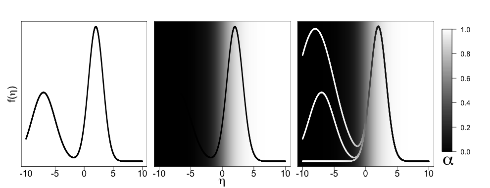
Figure 1: Left panel: a generic density $f^{*}(\eta)$. Center panel: same density as in left panel, but with background shading proportional to $\varphi^{-1}(\eta)$ with $\varphi$ the logit function. Right panel: several possible densities that share the same shape in the “observable” region, but different shapes in the “unobservable” region.

3 Estimation of $\alpha$-observable populations

We now introduce an alternative inferential approach that estimates the $\alpha$-observable population size $N_{\alpha}$ rather than the total population size $N$. Definition 3.1 formalizes the concept of $\alpha$-observability.

Definition 3.1.

Individual $i$ is $\alpha$-observable if $1-\pi_{\zeta,i}=p_{i}>\alpha$. We define the $\alpha$-observable population size, $N_{\alpha}$, as $N_{\alpha}=\sum_{i=1}^{N}\mathbbm{1}\left\{p_{i}>\alpha\right\}$. We call $[\alpha,1]$ the $\alpha$-observable region. Any set such that $A\subset[\alpha,1]$ is an $\alpha$-observable set. Any set that is not $\alpha$-observable is $\alpha$-unobservable.

In contrast to estimating $N$, estimating $N_{\alpha}$ requires learning the distribution $F$ only on $[\alpha,1]$. Then the analogue of $\widehat{N}$ is ^N_α = m_α {1-F(α)} {E_F(P)}^-1 = m_α {E_F_α(P)}^-1, where $m_{\alpha}$ is the number of observed individuals having $p\in\mathbb{[}\alpha,1]$ and $E_{F_{\alpha}}(P)=E_{F}(P\mid P>\alpha)$. So to estimate $\widehat{N}_{\alpha}$ we only need to integrate over $[\alpha,1]$, not the entire unit interval.

3.1 Risk of estimators of $N$ and $N_{\alpha}$

We now show that estimators of $N_{\alpha}$ have lower risk than estimators of $N$. Intuitively, low risk of any nonparametric estimator $\widehat{F}$ of $F$ requires that we observe data with high probability in sets whose $F$ measure is bounded away from zero. We refer to these sets as non-negligible.

Definition 3.2 (Non-negligible sets).

For any $\epsilon>0$, a Borel set $A$ is non-negligible with respect to $F$ and $\epsilon$ if $\int_{p\in A}F(dp)>\epsilon$.

Theorem 3.3 shows that we can guarantee a uniform minimal probability of observing data in non-negligible $\alpha$-observable sets in finite samples, but not in all non-negligible sets. Therefore, nonparametric estimators of $N_{\alpha}$ are expected to have better finite-sample performance than estimators of $N$. All proofs are deferred to the Appendix.

Theorem 3.3 (Finite sample bounds in $\alpha$-observable populations).

Suppose the true population size is $N$ and fix $\epsilon>0$. Let $\mathcal{A}$ be the set of all $(F,\epsilon)$ non-negligible $\alpha$-observable intervals, and for any $A\subset\mathbb{[}0,1]$, let $M(A):=\sum_{i:p_{i}\in A}\mathbbm{1}\left\{\sum_{t=1}^{T}x_{it}>0\right\}$, the number of observations with $p\in A$. Then

$$\inf_{A\in\mathcal{A}}\mathrm{pr}\{M(A)>0\}=1-(1-\alpha\epsilon)^{N}.$$ (1)

That is, for fixed $N$, the probability that some data are observed in any non-negligible set is bounded below by the right hand side of (1), which is a function of $\alpha$. For $\alpha=0$, the only uniform bound is the trivial bound $\inf_{A\in\mathcal{A}}\mathrm{pr}\{M(A)>0\}=0$. Another implication of Theorem 3.3 is that for fixed $\alpha$ and $\epsilon$ and any $q\in(0,1)$, there exists $N<\infty$ large enough that the probability of observing data in $A\in\mathcal{A}$ is uniformly bounded below by $q$. Of course, no finite value of $N$ would be sufficient to guarantee a uniform lower bound on the probability of observing data in an arbitrary non-negligible subset of the unit interval. Finally, Theorem 3.3 suggests one approach for choosing values of $\alpha$ based on the number of unique observed individuals $m$. Although $N$ is unknown, it is always the case that $N\geq m$, so the probability of observing data in non-negligible $\alpha$-observable sets can be lower-bounded by (1) with $N=m$. Therefore, one way to assess different choices of $\alpha$ is to compute (1) for the observed population size $m$ and a range of $\epsilon$ values.

Now we consider the risk of estimators of $N$ and $N_{\alpha}$. Throughout, we will assume that we observe directly length-biased data proportional to $pF(dp)$. In capture-recapture applications, $p$ is latent, so the results in this section provide a lower bound on the risk of capture-recapture estimates of $N$. The distribution of the observed data is G(dp) = p F(dp)Ef(P), since $G(dp)$ must integrate to 1. Consider an estimator $\widehat{G}$ of $G$. We propose to use ^F(dp) = p-1^G(dp)E^G(P-1) as an estimator of $F$. This is similar to the approach in hatjispyros2015bayesian. This estimator is appropriate in at least one sense, which is to say that since $F(dp)\propto p^{-1}\,G(dp)$, it must be the case that F(dp) = p-1G(dp)EG(P-1) = p^-1 G(dp) E_f(P), so $E_{G}(P^{-1})=\{E_{F}(P)\}^{-1}$, and $\widehat{F}$ is the plug-in estimator of $F$ derived from any estimator of the observable distribution $\widehat{G}$.

We now consider two procedures for estimation of $\widehat{G}$. Critically, when $F$ is unknown, we cannot estimate $E_{F}(P)$ without implicitly choosing an estimator $\widehat{F}$ because of the length bias in the observed data. We consider two possible estimators of $\widehat{G}$: the empirical measure and a histogram estimator. These estimators are classical analogues of the Bayesian Dirichlet process model we propose in §LABEL:sec:dp. Since $E_{G}(P^{-1})=\{E_{F}(P)\}^{-1}$, in either case the estimator $\widehat{N}$ is given by $mE_{\widehat{G}}(P^{-1})$. When $\widehat{G}$ is the empirical measure, this is just the sample mean of $p^{-1}$, $\widehat{N}=\sum_{i=1}^{m}p_{i}^{-1}$, and we have the following result for the mean squared error of $\widehat{N}$.

Theorem 3.4 (Mean squared error for empirical measure estimator).

If $\widehat{G}(dp)=\sum_{i=1}^{m}\delta_{p_{i}}(dp)$ then the mean squared error $\Delta^{2}(\widehat{N},N)$ is given by Δ^2(^N,N) = N { E_F(P^-1) - 1 }.

It is immediate that for $\Delta^{2}(\widehat{N},N)<\infty$, we need $E_{F}(P^{-1})<\infty$. In many seemingly mundane cases this fails, for example when $F$ is a $\text{Beta}(a,b)$ distribution with $a\leq 1$, which includes the uniform distribution on the unit interval. The following Corollary shows that the empirical measure estimator of $N_{\alpha}$ always has finite $L_{2}$ risk, and the risk decreases with increasing $\alpha$.

Corollary 3.5 (Mean squared error for empirical measure estimator of $N_{\alpha}$).

For any $\alpha\in(0,1]$ if $\widehat{N}_{\alpha}$ is the empirical measure estimator of $N_{\alpha}$, then Δ^2(^N_α,N_α) = N_α { E_F_α(P^-1) - 1 } ≤N_α (α^-1-1), and $N_{\alpha}^{-1}\Delta^{2}(\widehat{N}_{\alpha},N_{\alpha})$ is monotone nonincreasing in $\alpha$.

Finally, in many cases $\widehat{N}_{\alpha}$ using the empirical measure estimator of $F$ will have lower $L_{2}$ risk for $N$ than the corresponding empirical measure estimator of $N$, and $\widehat{N}$ cannot be a minimax estimator of $N$ in the nonparametric regime.

Corollary 3.6 (Mean squared error for estimation of $N$ by the empirical measure estimator of $N_{\alpha}$).

For any $\alpha\in(0,1]$ if $\widehat{N}_{\alpha}$ is the empirical measure estimator of $N_{\alpha}$, then Δ^2(^N_α,N) = N_α { E_F_α(P^-1) - 1 } + (N-N_α)^2 ≤N_α (α^-1-1) + (N-N_α)^2. Therefore, $\Delta^{2}(\widehat{N}_{\alpha},N)<\Delta^{2}(\widehat{N},N)$ whenever $N_{\alpha}\{E_{F_{\alpha}}(P^{-1})-1\}+(N-N_{\alpha})^{2}<N\{E_{F}(P^{-1})-1\}$. In particular, $\widehat{N}$ cannot be a minimax estimator of $N$ when $F$ is unknown, since there exists $F$ for which $\Delta^{2}(\widehat{N},N)=\infty$, while $\Delta^{2}(\widehat{N}_{\alpha},N)<\infty$ for all $F$.

We now consider the case where $F$ has a density $f$ and $\widehat{g}$ is the histogram estimator. The histogram estimator is a commonly used nonparametric density estimator. We have the following result for the risk of histogram-based estimators of $N$.

Theorem 3.7 (Mean squared error of histogram estimators of $N$).

Suppose $\widehat{g}$ is the histogram estimator with bin width $h$. Assume $f$ is twice continuously differentiable. Then the mean squared error $\Delta^{2}(\widehat{N},N)$ satisfies 0 ≤Δ^2(^N,N) - N [ E_f(P^-1) - {E_f(P)}^-1 ] + O ( Nh ) ≤N2h24 { E_f(P^-1) + E_f{—f’(P)—} }^2 Further, the asymptotic variance (as $n\to\infty$ and $h\to 0$) of $\widehat{N}$ is given by $N\left[E_{f}(P^{-1})-\{E_{f}(P)\}^{-1}\right]$, and the asymptotic bias is bounded above by $(N^{2}h^{2}/4)\left\{E_{f}(P^{-1})+E_{f}\{|f^{\prime}(P)|\}\right\}^{2}$.

From equation (3.7), it is clear that when $h$ shrinks faster than $N^{-1/2}$, the asymptotic mean squared error and asymptotic variance are identical. Moreover, for twice differentiable densities $f$, we can improve upon the asymptotic mean squared error for the empirical measure estimator, since $\{E_{F}(P^{-1})-1\}\geq[E_{f}(P^{-1})-\{E_{f}(P)\}^{-1}]$. Nonetheless, $\Delta^{2}(\widehat{N},N)<\infty$ still requires $E_{f}(P^{-1})<\infty$. The following Corollary shows that estimating $N_{\alpha}$ has similar benefits when we use a histogram estimator of $g$.

Corollary 3.8 (Mean squared error of histogram estimators of $N_{\alpha}$).

Under the conditions of Theorem 3.7, if $\alpha\in(0,1]$ and $h=N^{-(1+\delta)/2}$ for $\delta>0$ then lim_N_α →∞ N_α^-1 Δ^2(^N_α,N_α) = [ E_f_α(P^-1) - {E_f_α(P)}^-1 ] ¡ α^-1. Furthermore, if $E_{f_{\alpha}}(P^{-1})-\{E_{f_{\alpha}}(P)\}^{-1}$ is monotone nonincreasing in $\alpha$, then the asymptotic mean squared error of $\widehat{N}_{\alpha}$ is also monotone nonincreasing in $\alpha$.

We conjecture that $E_{f_{\alpha}}(P^{-1})-\{E_{f_{\alpha}}(P)\}^{-1}$ is monotone nonincreasing in general, though something stronger than the obvious convexity argument is required to show this result. Empirically, this holds for all of the distributions we have tested. We also have a result similar to Corollary 3.6 for the histogram estimator.

Corollary 3.9 (Mean squared error for estimation of $N$ by histogram estimator of $\widehat{N}_{\alpha}$).

For any $\alpha\in(0,1]$ if $\widehat{N}_{\alpha}$ is the histogram estimator of $N_{\alpha}$ and the conditions of Theorem 3.7 hold, then Δ^2(^N_α,N) &≤Δ^2(^N_α,N_α) + (N-N_α)^2 ¡ ∞It follows that $\widehat{N}$ cannot be a minimax estimator of $N$ when $F$ is unknown, since there exists $F$ for which $\Delta^{2}(\widehat{N},N)=\infty$, while $\Delta^{2}(\widehat{N}_{\alpha},N)<\infty$ for all $F$.

Theorems 3.4 and 3.7 show that in many cases, estimators of $N$ have unbounded risk, while Corollaries 3.5 and 3.8 guarantee that for any $\alpha>0$, there exist estimators of $N_{\alpha}$ with finite risk for any $F$. Further, these results imply that the choice of $\alpha$ can be viewed as a tradeoff between higher mean squared error and estimating a quantity closer to the total population size. Finally, Corollaries 3.6 and 3.9 show that estimators of $N_{\alpha}$ often have lower risk for estimation of $N$ than the corresponding estimators of $N$ and are superior in the minimax sense. These are the basic lessons that motivates the methods we propose for estimation of $N_{\alpha}$ and choice of $\alpha$ in the sequel.

4 Model-based estimation of $N_{\alpha}$

Thus far, the discussion has centered on $p_{i}=1-\pi_{\zeta,i}$ without specifying a model for the other cell probabilities. In capture-recapture, we must use the data on presence or absence on the $T$ lists to estimate the latent distribution $F$ and the population size $N$. This is generally done by specifying a model on the individual-level cell probabilities $\pi_{x,i}$, which induces a model on $p_{i}=1-\pi_{\zeta,i}$, and on $F$ by marginalizing over individuals. We now restrict our attention to a specific class of such models, the $M^{th}$ class. In modeling, it is common to parametrize probabilities via a monotone nondecreasing transformation $\varphi^{-1}:\mathbb{R}\to[0,1]$, such as the logit or probit function. We will follow this convention for the remainder of the paper, and will write $\eta=\varphi(p)$ for the transformed individual observabilities. Densities and distribution functions supported on the real line induced by the transformation of $P\sim F$ via $\varphi$ are represented with superscript ^∗, for example, $f^{*}(\eta)$ and $F^{*}$.

4.1 $M^{th}$ Model

The $M^{th}$ model (Agresti1994) is given by the following joint distribution for the list capture random variables $X_{1},\ldots,X_{T}$: pr ( X_i1=x_1,…,X_iT=x_T ∣θ, β ) &= ∏_t=1^T φ^-1(θ_i + β_t)^x_it {1-φ^-1(θ_i + β_t)}^1-x_it,  θ_i ∼iid G^*, where the $\theta_{i}$ are individual-specific observability effects distributed according to a distribution $G^{*}$ supported on $\mathbb{R}$, and the $\beta_{t}$ are global list effects. By (4.1), individual $i$ is $\alpha$-observable in this model if p_i= φ^-1(η_i) = 1-∏_t=1