The Politics of Routing: Investigating the Relationship Between AS Connectivity and Internet Freedom

Abstract

The Internet’s importance for promoting free and open communication has led to widespread crackdowns on its use in countries around the world. In this study, we investigate the relationship between national policies around freedom of speech and Internet topology in countries around the world. We combine techniques from network measurement and machine learning to identify features of Internet structure at the national level that are the best indicators of a country’s level of freedom. We find that IP density and path lengths to other countries are the best indicators of a country’s freedom. We also find that our methods predict freedom categories for countries with 91% accuracy.

1 Introduction

The Internet’s role as a communication tool for activists and dissidents has led to increasing efforts on the part of nation states to restrict access and control information accessed online [5]. These efforts to clamp down on Internet freedom can lead to national policies that influence the interdomain topologies of given countries (e.g., Iran’s policy that all networks must connect via the national telecom AS 12880 [2]) and the topologies in turn can make certain forms of information control easier (e.g., country-wide Internet shut downs [7]).

In this study, we consider the relationship between interdomain topology–i.e., routing between autonomous systems (ASes)–and Internet freedom in countries around the globe. We use a combination of standard graph theoretic metrics and domain-specific features to understand how these features relate to Internet freedom, which we quantify using the Freedom House Freedom of the Press index [8]. Our goal is to understand the way that online information controls can impact the network topology of different countries as well as which topologies are more likely to facilitate restrictions on Internet access. Understanding this relationship can help fill in gaps in existing data sets about Internet freedom, many of which require manual effort and measurement points within the region to compute. By looking at the interdomain topologies we can understand which countries are similar in terms of network structure and identify regions that warrant more investigation. Further, by understanding network properties that correlate with information controls we can potentially identify countries that are in a good position to perform filtering or Internet shutdowns and see the legacy effects after filtering has been repealed. While it may seem simple, studying the interdomain topology around the globe requires care to avoid known blind spots in existing data. We perform traceroutes using RIPE Atlas [12] to expose additional edges in and around different countries (§2.2). We use a state-of-the-art BGP path simulator  [10] which allows us to consider graph theoretic metrics with paths that incorporate routing policy vs. simple shortest path. We combine our empirically derived data with existing AS-level topologies [6] to characterize the interdomain topologies of countries around the globe. We consider a variety of structural features and domain specific features and characterize their relationship to free communication and find that the number of IP addresses per individual (IP density) is the most important predictor of Internet freedom(§4). We leverage these features and machine learning techniques to group countries based on their interdomain topologies (§3.2).

2 Internet Topology Data Sets

In this section, we provide background on the Internet topology and describe our methodology for improving the fidelity of existing data sets.

2.1 Initial Topology

Central to our approach are graphs of the Internet topology of each country. These graphs are empirically derived and are comprised of autonomous systems (ASes) as nodes and connections between them as edges. An AS generally represents a network under the control of a single entity (e.g., an ISP, university or business). Each edge is annotated with the inferred business relationship between the two ASes it connects (i.e., who pays who). Figure 1 illustrates an example topology where AS 1 is a customer of AS 2 and pays it for transit and AS 2 and AS 3 are settlement-free peers exchanging traffic at no cost. We start from the AS graph published by CAIDA [6] which includes all observed ASes and is labeled with inferred business relationships [11].

Figure 1: AS relationships on the Internet

Since ASes may span multiple countries and even continents, we make a simplifying assumption and consider an AS to belong to the country it is registered in. We determine where each AS in the topology is registered using datasets from the regional Internet registries (RIRs).

2.2 Increasing Coverage

A key challenge we face in this work, is contending with known incompleteness of existing AS-level topologies. Specifically, edges close to the network edge, particularly settlement-free peering edges are particularly hard to observe. Further, the bulk of data for Internet topology mapping is derived from BGP monitors that tend to be located in the Americas, Europe and Asia vs. the Middle East, Africa and other regions known to be implementing online information controls. We use the RIPE Atlas platform [12] and perform targeted traceroutes to uncover these missing edges.

We focus on illuminating two key types of connectivity: (1) international connectivity of each country and (2) domestic connectivity of the countries. We devise two tracerouting strategies to uncover these two types of edges.

Inside-out and Outside-in. In order to find undiscovered international edges from a country, we need to traceroute from domestic sources to international destinations and vice versa (we call these traceroutes “Inside-Out” and “Outside-in”). We perform traceroutes from a set of domestic RIPE Atlas probes to a randomly selected set of international probes for each country. This technique of measuring “Inside-Out” exposes links that are used by traffic flowing out of the country. Similarly, we perform traceroutes from the randomly selected international probes to the set of domestic probes (measuring “Outside-In”). The size of the subset of probes (both domestic probes and international) is progressively increased, starting from 5, in steps of 5 until no new edges are seen in 3 consecutive sets of measurements.

Mesh. For discovering new edges local to the country (domestic edges connect two domestic ASes), we traceroute from a domestic source to a domestic destination (we call these traceroutes “Mesh traceroutes” since they are between all pairs of domestic traceroute vantage points, forming a mesh).

Mapping traceroutes back to AS paths. We take care when converting our new traceroute measurements to AS paths. Specifically, we use a list of prefixes belonging to Internet eXchange Points (IXPs) published by PeeringDB [4] to identify and remove IP hops in our traceroutes that are located in IXPs. After removing hops in IXPs, we use CAIDA’s IP prefix to ASN mapping [1] to convert the traceroute to an AS-level path.

Inferring relationships. Inferring business relationships between ASes is a challenging problem and open area of research. We take the following approach to infer business relationships on new edges discovered via our traceroute measurements. We begin by retrieving the inferred relationships for any edges that appear in our traceroute and in the existing dataset from CAIDA. We use these inferred relationships combined with the assumption that ASes will only transit traffic between two neighboring ASes if at least one of these neighbors is a customer (the “valley free” assumption) to constrain the business relationship for a given edge.

Table 1 summarizes the new edges found using the two methods described above. From the table it is clear that domestic mesh traceroutes were the most beneficial, exposing a total of 5,562 new edges. Further, the benefit of adding more probes to the Inside-out traces begins to level off around 25 probes. Table 2 summarizes the countries that benefited most from the additional measurements and the number of new edges uncovered in each case.

Measurement Type	Total New AS edges
I/O with 5 probes	85
I/O with 10 probes	180
I/O with 15 probes	334
I/O with 20 probes	509
I/O with 25 probes	647
Domestic mesh	5,562

Table 1: Benefit of measurements in terms of newly discovered AS edges (I/O represents Inside-out/Outside-in traceroutes).

Country	Total AS edges
RU	957
US	547
FR	443
GB	441
UA	304

Table 2: Top countries in terms of new edges.

3 AS Topology and Internet Freedom

We study the connection between the AS-level topology derived in the previous section and the freedom of information in a given country. The Freedom House Freedom of the Press Index (FPI), lying between 0 (high freedom) and 100 (low freedom), serves as a proxy for the freedom of information in a country. Our approach is to use features extracted from AS-level topologies as input to machine learning methods to predict $100-\textrm{FPI}$ as the target metric, which has a higher value for a higher degree of freedom.

In this section, we describe the features and machine learning methods that we use in our approach. We evaluate the accuracy of these methods in §3.3.

3.1 Features of the AS topologies

For each AS-level topology, we compute a set of features and meta-information. We break these features into four broad categories. Below, we briefly describe each class with a few examples; Table 3 enumerates the complete set of features considered.

1. Structural Features. This includes features of the AS-graph related to its structure such as the number of nodes or edges and connectivity features.

2. International Connectivity Features This include features related to how a country connects to networks in other countries. Specifically, how many countries and networks does it connect to and what are its path lengths to other countries.

3. IP Demographic Features. This captures how much of the IP address space does the country control. It also considers the relationship between IP space and the population of the countries (i.e., how many IPs are there per person).

4. BGP Routing Features. This includes features related to properties of ISPs and networks in the country. We consider the counts of small stub networks, large providers, and percentiles of the customer cone size of networks in the country.

Preprocessing the features. Since the values of different features lie in different ranges, we scale each feature using min-max scaling:

$$\hat{X}=\frac{X-X_{min}}{X_{max}-X_{min}}$$ (1)

Where $\hat{X}$ is the scaled value for a feature with original value X. $X_{min}$ and $X_{max}$ are the minimum and maximum values of that feature across all countries. After scaling, all features lie in the range (0,1). However we observe a number of outliers in the feature values. To mitigate their effect on our prediction we removed the countries with outlier features from the training data. As a result, we removed US, RU, SC and NL from the training data. The AS graphs of RU and US are much larger than the other countries. In case of NL, the presence of IXPs biases features relating to AS relationships (like the number of peering edges). SC has an IP density value magnitudes higher than all other countries.

Table 3: Feature categories and description

Features of Countries
Category	Name	Description
Structural Features	$f_{1}$: num_nodes	Number of nodes in the country’s graph
	$f_{2}$: num_edges	Number of edges in the country’s graph
	$f_{3}$: percentile_degree	$95^{th}$ percentile of the node degrees in the graph
	$f_{4}$: diameter	Diameter of the country’s AS graph
	$f_{5}$:avg_h_im	Average horizontal imbalance
	$f_{6}$: max_load_cen	Maximum load centrality of a node in the AS graph
	$f_{7}$: avg_clustering	Average clustering coefficient of the graph
	$f_{8}$: graph_clique_number	Size of the largest clique in the graph
	$f_{9}$: alg_conn	AUC of decay of algebraic connectivity as nodes are removed in order of AS rank
	$f_{10}$: frac_conn	AUC of decay of fraction of largest connected component as nodes are removed in order of AS rank
	$f_{11}$: transitivity	the fraction of all possible triangles present in the graph
	$f_{12}$: num_large_nodes	Number of nodes in the graph with degree
International Connectivity Features	$f_{12}$: max_path_len	maximum length of routed paths from a given country to all other countries
	$f_{13}$: num_intl_countries	Number of countries, a country directly connects to
	$f_{14}$: num_intl_nodes	Number of nodes providing international connectivity
IP Demographic Features	$f_{15}$: ip_density	Number of IPs per person
	$f_{16}$: num_announced_ip	Number of prefixes announced by the country
BGP Routing Features	$f_{17}$: num_large_providers	Number of ASes with customer cone size >100
	$f_{18}$: percentile_cust_cone	95th percentile of the customer cone sizes in the country
	$f_{19}$: stub_ases	Number of stub ASes
	$f_{20}$: tot_peer_edges	Number of AS edges in the graph that are p2p

3.2 Predicting Freedom of the Press Index (FPI)

We predict the FPI for 170 countries using these features. We consider four different machine learning models of increasing complexity for this task. We note that our methods automatically account for the features that do not individually correlate with FPI.

Linear Regression (LR). We used the features to train a linear regression model. This method finds a linear function of the features that best predicts the FPI. This type of method performs well when the target variable is a globally linear function of the features.

Regularised Linear Regression (LASSO). Due to the small number of data points, the LR model may overfit in the face of many features. To avoid overfitting, we make use of LASSO (Least Absolute Shrinkage and Selection Operator) that shrinks dimensionality by selecting the most predictive features trying to jointly minimize prediction loss as well as L1-norm of the feature space.

In addition to the linear models, we consider decision tree-based approaches. The advantage of these approaches is that they are non-linear and divide the dataset into groups that are similar with respect to the features. The prediction function within each group is then decided as part of the model design.

Decision Tree with simple averaging at the leaves (DTLA) We train a decision tree model that groups similar countries in a group. We predict the FPI of countries in the same bucket by taking an average of actual FPI values in the group.

Decision Tree with Linear Regression at leaves (DTLR) This model is similar to the last one. However, instead of predicting the FPI for a group based on its average, a linear regression is run within each group to predict the FPI values. We note that we only perform the linear regression in groups that have size at least 10; for the remaining groups we take the average (as in the previous approach). The prediction function within each leaf is then decided as part of the model design

3.3 Evaluating Predicted FPIs

We evaluate the four models described above using the 170 countries present in the 2012 FPI values for which it was possible to compute the features described in Table 3. We use leave-one-out cross validation (LOOCV) to evaluate the ML methods. We train each of the 4 models (LR, LASSO, DTLA, DTLR) with all but one country and then evaluate how well we predict the leftout country. This process is repeated in turn for all 170 countries.

Predicting FPI. Figure 3 shows the estimated kernel density function for the distribution of prediction errors for each of the four aforementioned models. We find LR and LASSO that perform linear regression across the entire dataset, provide poor accuracy with an average prediction error of 15.05%. The decision tree model (DTLA) has modestly increased accuracy but the average prediction error reamined close to 15.04%. Performing linear regression within the groups produced by the decision tree (DTLR) has the highest accuracy with an average prediction error of 7.06%.

Figure 4 shows the cumulative distributon of normalized error (i.e., $\frac{predictedFPI}{actualFPI}$) for the four models. We note that the best model–decision tree with linear regression–has an error of atmost 10%, 71% of the time.

Predicting freedom category. Freedom House groups countries based on their FPI value: ($61-100$) Free, ($31-60$) Partly-Free, and ($0-30$) Not Free. We also consider how well our model predicts the category a country will fall under. By discretizing the predictions of DTLR, we were able to predict the freedom categories with 81% accuracy. The countries for which DTLR predicted freedom category wrongly, often, our prediction and the actual freedom category were partly-free and free (and vice versa). If we consider free and partly-free as the same label, our accuracy of prediction improves to 91%.

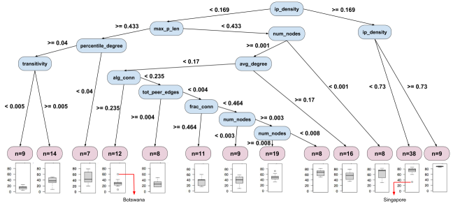
Figure 2: Comparison of the prediction error of our learning approaches. Arrow point to local outliers, see Section 5 for details

Figure 3: Comparison of the prediction error of our learning approaches.

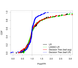
Figure 4: CDF of the prediction error of our learning approaches.

4 Features that Predict Freedom

We now discuss which features are the most relevant for predicting FPI using our most accurate classification model (decision tree with linear regression).

IP density has the highest influence on the freedom index. As Figure 2 shows, a normalised IP density value of 0.169 or higher implies high freedom of expression in a country. This metric captures the ratio of IP addresses to users within a country and can be seen as approximating the level of connectivity per capita in the country.

We also observe a negative correlation between the maximum length of BGP policy compliant paths from a country to all other countries (max_p_len). Normalised max_p_len value of 0.433 or lower ensures high freedom in a country. This makes intuitive sense since longer paths imply poor connectivity.

We find that poor connectivity properties tend to correspond to countries with low FPI values. Countries with high path length, low degree values and low transivity (i.e., number of “triangles” in the graph) are among the lowest in terms of FPI scores. This first group includes countries that are known to implement strong information controls (e.g., Ethiopia, China, Cuba).

(a) Singapore

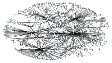
(b) Iran

Figure 5: AS graphs for Singapore and Iran (red/dark nodes are international ASes and light nodes are domestic.

5 Identifying Unusual Countries

Our decision tree can also highlight countries with connectivity profiles that are not consistent with their information control policies. There two such instances that stand out in Figure 2: Botswana and Singapore. In case of Singapore, according to our prediction the FPI should be very high ($\>80$). But in reality the FPI index of SG is 31. On the other hand, our FPI prediction for Botswana is very low (29.25) but in reality Botswana has high freedom of expression.

We dig deeper into the case of Singapore. Singapore respresents a country with a well established IT infrastructure that also implements online information controls [3]. We can see this difference qualitatively in Figure 5 which compares the connectivity graphs of Singapore and one of the least free countries, Iran. Iran shows strong limits in terms of international connectivity, connecting to only three international networks. Singapore, in contrast, has a rich international connectivity with 257 domestic ASes connecting to a total of 3022 international ASes.

6 Conclusions

Freedom House FPI assesses the degree of freedom in digital and print media for countries across the globe. Using FPI as a measure of freedom of expression, we investigate the relationship between Internet infrastructure and information freedom around the globe. Our techniques can help bootstrap understandings of information freedom when empirical data may not be readily available. We are also able to identify features of AS topologies that are more representative of countries that implement online information controls.

Future work. While this work presents a first exploration of the relationship between Internet infrasturcture and information freedom, there is still much ground to be covered in this space. In future work, we plan to take a two pronged approach to extend this study. Specifically, we hope to leverage social science expertise to better reason about the social and political factors that impact information policy and discuss our findings with operators of existing large networks to see how policy shapes their day-to-day network management.

References

- [1] Caida’s prefix to asn dataset. https://www.caida.org/data/routing/routeviews-prefix2as.xml.
- [2] ONI Report Iran. https://opennet.net/research/profiles/iran.
- [3] ONI Report Singapore. https://opennet.net/research/profiles/singapore.
- [4] PeeringDB. https://www.peeringdb.com/.
- [5] What Was the Role of Social Media During the Arab Spring? https://www.library.cornell.edu/colldev/mideast/Role%20of%20Social%20Media%20During%20the%20Arab%20Spring.pdf.
- [6] CAIDA AS Relationship dataset. http://data.caida.org/datasets/as-relationships/.
- [7] A. Dainotti, C. Squarcella, E. Aben, K. C. Claffy, M. Chiesa, M. Russo, and A. Pescapé. Analysis of country-wide internet outages caused by censorship. In Proceedings of the 2011 ACM SIGCOMM conference on Internet measurement conference, pages 1–18. ACM, 2011.
- [8] Freedom of the Press by Freedom House. https://freedomhouse.org/report-types/freedom-press.
- [9] Freedom on the Net by Freedom House. https://freedomhouse.org/report-types/freedom-net.
- [10] P. Gill, M. Schapira, and S. Goldberg. Modeling on quicksand: Dealing with the scarcity of ground truth in interdomain routing data. ACM SIGCOMM Computer Communication Review, 42(1):40–46, 2012.
- [11] V. Giotsas, M. Luckie, B. Huffaker, and k. claffy. Inferring Complex AS Relationships. In Internet Measurement Conference (IMC), pages 23–30, Nov 2014.
- [12] RIPE Atlas. https://atlas.ripe.net/.