Efficient differentially private learning improves drug sensitivity prediction

Abstract

Users of a personalised recommendation system face a dilemma: recommendations can be improved by learning from data, but only if the other users are willing to share their private information. Good personalised predictions are vitally important in precision medicine, but genomic information on which the predictions are based is also particularly sensitive, as it directly identifies the patients and hence cannot easily be anonymised. Differential privacy [7, 8] has emerged as a potentially promising solution: privacy is considered sufficient if presence of individual patients cannot be distinguished. However, differentially private learning with current methods does not improve predictions with feasible data sizes and dimensionalities [10]. Here we show that useful predictors can be learned under powerful differential privacy guarantees, and even from moderately-sized data sets, by demonstrating significant improvements with a new robust private regression method in the accuracy of private drug sensitivity prediction [4]. The method combines two key properties not present even in recent proposals [26, 9], which can be generalised to other predictors: we prove it is asymptotically consistently and efficiently private, and demonstrate that it performs well on finite data. Good finite data performance is achieved by limiting the sharing of private information by decreasing the dimensionality and by projecting outliers to fit tighter bounds, therefore needing to add less noise for equal privacy. As already the simple-to-implement method shows promise on the challenging genomic data, we anticipate rapid progress towards practical applications in many fields, such as mobile sensing and social media, in addition to the badly needed precision medicine solutions.

1 Introduction

The widespread collection of private data, both by individuals and hospitals in the health domain, creates a major opportunity to develop new services by learning predictive models from the data. Privacy-preserving algorithms are required and have been proposed, but for instance anonymisation approaches [1, 18, 17] cannot guarantee privacy against adversaries with additional side information, and are poorly suited for genomic data where the entire data is identifying [13]. Guarantees of differential privacy [7, 8] remain valid even under these conditions [8], and differential privacy has arisen as the most popularly studied strong privacy mechanism for learning from data.

2 Efficient differentially private learning

Differential privacy [7, 8] is a formulation of reasonable privacy guarantees for privacy-preserving computation. It gives guarantees about the output of a computation and can be combined with complementary cryptographic approaches such as homomorphic encryption [12] if the computation process needs protection too. An algorithm $\mathcal{M}$ operating on a data set $\mathcal{D}$ is said to be differentially private if for any two data sets $\mathcal{D}$ and $\mathcal{D}^{\prime}$, differing only by one sample, the ratio of probabilities of obtaining any specific result $c$ is bounded as

$$\frac{p(\mathcal{M}(\mathcal{D})=c)}{p(\mathcal{M}(\mathcal{D}^{\prime})=c)}\leq\exp(\epsilon).$$ (1)

Because of symmetry between $\mathcal{D}$ and $\mathcal{D}^{\prime}$ the probabilities need to be similar to satisfy the condition. Differential privacy is preserved in post-processing, which makes it flexible to use in complex algorithms. The $\epsilon$ is a privacy parameter interpretable as a privacy budget, with higher values corresponding to less privacy preservation. Differentially private learning algorithms are usually based on perturbing either the input [2, 7], output [7, 26] or the objective [3, 28].

Here we apply differential privacy to regression. The aim is to learn a model to predict the scalar target $y_{i}$ from $d$-dimensional inputs $x_{i}$ (Fig. 1a) as $y_{i}=f(x_{i})+\eta_{i}$, where $f$ is an unknown mapping and $\eta_{i}$ represents noise and modelling error. We wish to design a suitable structure for $f$ and a differentially private mechanism for efficiently learning an accurate private $f$ from a data set $\mathcal{D}=\{(x_{i},y_{i})\}_{i=1}^{n}$.

We argue that a practical differentially private algorithm needs to combine two things: (i) it needs to provide asymptotically efficiently private estimators so that the excess loss incurred from preserving privacy will diminish as the number of samples $n$ in the data set increases; (ii) it needs to perform well on moderately-sized data.

While the first requirement of asymptotic efficiency or consistency seems obvious, it is non-trivial to implement in practice and rules out some mechanisms published even quite recently [29]. The requirement was addressed in the Bayesian setting very recently [9], but the method failed to cover the second equally important criterion. Asymptotically consistently private methods always allow reaching stronger privacy with more samples.

It is difficult to prove optimality of a method on finite data so good performance needs to be demonstrated empirically. A design strategy for good methods controls the amount of shared private information. This has two components: (a) dimensionality needs to be reduced, to avoid the inherent incompatibility of privacy and high dimensionality which has been discussed previously [6], and (b) introducing robustness by bounding and transforming each variable (feature) to a tighter interval. Controlling the amount of shared information also introduces a trade-off: compared to the non-private setting, decreasing the dimensionality a lot may degrade the performance of the non-private approach, while a corresponding low-dimensional private algorithm may attain higher performance than a higher-dimensional one (see the results and Fig. 3a).

The essence of differential privacy is to inject a sufficient amount of noise to mask the differences between the computation results obtained from neighbouring data sets (differing by only one entry). The definition depends on the worst-case behaviour, which implies that suitably limiting the space of allowed results will reduce the amount of noise needed and potentially improve the results. In the output perturbation framework this can be achieved by bounding the possible outputs [26].

Here we propose a more powerful approach of bounding the data by projecting outliers to tighter bounds. The current standard practice in private learning is to linearly transform the data to desired bounds [28]. This is clearly sub-optimal as a few outliers can force a very small scale for other points. Significantly higher signal-to-privacy-noise ratio can be achieved by setting the bounds to cover the essential variation in the data and projecting the outliers separately inside these bounds. This approach also robustifies the analysis against outliers as the projection can be made independent of the outlier scale. In linear regression we call the resulting model robust private linear regression. It is illustrated in Fig. 1b, c.

a
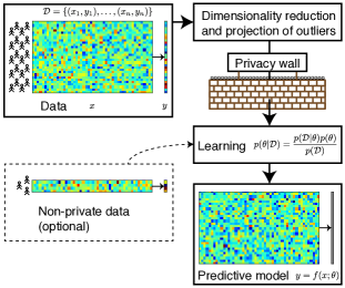
c b

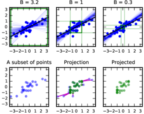
Figure 1: Differentially private learning of a predictive model. a, The modelling setup; most data (top) are available for learning only if their privacy can be protected. b, Bounding the data increasingly tightly (B; green square) brings 1D robust private linear regression models (blue lines illustrating the distribution of results of the randomised algorithm) closer to the non-private model (black line) as less noise needs to be injected. Blue points: data. c, The data are bounded in robust private linear regression by projecting outliers within the bounds (shown only for a subset of the points).

3 Results

Genomics is an important domain for privacy-aware modelling, in particular for precision medicine. Many people wish to keep their and also their relatives’ genomes private [19], and simple anonymisation is not sufficient to protect privacy since a genome is inherently identifiable [13]. Furthermore, individual genomes can be recovered from summary statistics [15] as well as phenotype data such as gene expression data [14]. On the other hand, previous research has shown that poorly implemented private models may put a patient to severe risk [10].

We apply the robust private linear regression model to predict drug sensitivity given gene expression data, in a setup where a small internal data set can be complemented by a larger set only available under privacy protection (Fig. 1a). We use data from the Genomics of Drug Sensitivity in Cancer (GDSC) project [27], and the setting and evaluation are similar as in the recent DREAM-NCI drug sensitivity prediction challenge [4]. The sensitivity of each drug is predicted with Bayesian linear regression based on expression of known cancer genes identified by the GDSC project [27] to limit the dimensionality. We achieve differential privacy by injecting noise to the sufficient statistics computed from the data, using the Laplace mechanism [7]. Full details are presented in Methods.

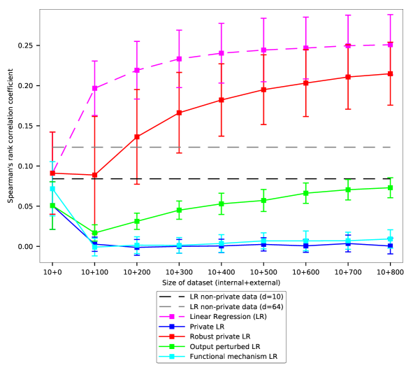
Figure 2: Accuracy of drug sensitivity prediction in terms of Spearman’s rank correlation coefficient over ranking cell lines by sensitivity to a drug (higher is better) increases with size of private data for the proposed robust private linear regression. The state-of-the-art methods fail to utilise private data under strict privacy conditions. The baselines (horizontal dashed lines) are learned on 10 non-private data points; the private algorithms additionally have privacy-protected data (x-axis). The non-private algorithm (LR) has the same amount of additional non-privacy-protected data. All methods use 10-dimensional data except purple baseline showing the best performance with 10 non-private data points. Private methods use $\epsilon=2$, corresponding results for $\epsilon=1$ are in Fig. 6. The results are averaged over all drugs and 50-fold Monte Carlo cross-validation; error bars denote standard deviation over 50 Monte Carlo repeats. (See Methods for details.)

Unlike with previous approaches, now prediction accuracy (ranking of new cell lines [4] to sensitive vs insensitive measured by Spearman’s rank correlation; Fig. 2) improves when more privacy protected data is received. The proposed non-linear projection of the data to tighter bounds is the key to this success, as without it the method performs as poorly as the earlier ones.

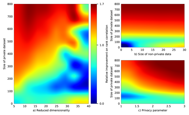
Figure 3: Key trade-offs in differentially private learning. Relative improvements over baseline (10 non-private data points). a, As the dimensionality increases, the models without private data improve whereas more data are needed to improve performance of the private methods. b, With enough private data, adding more non-private data does not significantly increase the performance. c, More data are needed if privacy guarantees are tighter ($\epsilon$ is smaller). Size of non-private data is 10 and $\epsilon=2$ (except when otherwise noted).

To improve prediction performance in differentially private learning, trade-offs need to be made between dimensionality and amount of data (Fig. 3a), and between strength of privacy guarantees and amount of data (Fig. 3c), but the amount of optional non-private data matters significantly only when there is very little private data (Fig. 3b).

In Secs. A–B in the Supplementary Information we define asymptotic consistency and efficiency of private estimators relative to non-private ones and prove that the optimal convergence rate of differentially private Bayesian estimators to the corresponding non-private ones is $\mathcal{O}(1/n)$ for $n$ samples, which is matched by our method. Unlike existing approaches [22, 24, 23], we compare the private estimators to the corresponding non-private ones, making the theory more easily accessible and more broadly applicable.

Robust private linear regression treats non-private and scrambled private data similarly in the model learning. An interesting next step for further improving the accuracy on very small private data would be to give a different weight to the clean and privacy-scrambled data by incorporating knowledge of the injected noise in the Bayesian inference, as has been proposed for generative models [25], but which is non-trivial in regression.

4 Methods

4.1 Linear regression model

The Bayesian linear regression model for scalar target $y_{i}$, with $d$-dimensional input $x_{i}$ and fixed noise precision $\lambda$, is defined by

$$y_{i}|x_{i} \sim N(x_{i}^{T}\beta,\lambda)$$

$$\beta \sim N(0,\lambda_{0}I),$$ (2)

where $\beta$ is the unknown parameter to be learnt. The $\lambda$ and $\lambda_{0}$ are the precision parameters of the corresponding Gaussian distributions, and act as regularisers.

Given an observed data set $\mathcal{D}=\{(x_{i},y_{i})\}_{i=1}^{n}$ with sufficient statistics $n\macc@depth\char 1\relax\frozen@everymath{\macc@group}\macc@set@skewchar\macc@nested@a 111{x}=\sum_{i=1}^{n}x_{i}x_{i}^{T}$ and $n\macc@depth\char 1\relax\frozen@everymath{\macc@group}\macc@set@skewchar\macc@nested@a 111{x}=\sum_{i=1}^{n}x_{i}y_{i}$, the posterior distribution of $\beta$ is Gaussian, $p(\beta|\mathcal{D})=N(\beta;\;\mu_{*},\Lambda_{*})$, with precision

$$\Lambda_{*}=\lambda_{0}I+\lambda n\macc@depth\char 1\relax\frozen@everymath{\macc@group}\macc@set@skewchar\macc@nested@a 111{x}$$ (3)

and mean

$$\mu_{*}=\Lambda_{*}^{-1}(\lambda n\macc@depth\char 1\relax\frozen@everymath{\macc@group}\macc@set@skewchar\macc@nested@a 111{x})$$ (4)

After learning with the training data set, the prediction of $y_{i}$ using $x_{i}$ is computed as follows:

$$\hat{y}_{i}=x_{i}^{T}\mu_{*}.$$ (5)

A more robust alternative is to define prior distributions for the precision parameters. In our case, a Gamma prior is assigned for both:

$$\lambda \sim\mathrm{Gamma}(a,b)$$

$$\lambda_{0} \sim\mathrm{Gamma}(a_{0},b_{0}).$$ (6)

The posterior can be sampled using computational methods such as automatic differentation variational inference (ADVI) [16] where we fit a variational distribution to the posterior. The precision parameters and correlation coefficients $\beta$ are then sampled from the fitted distribution. For this purpose, the data likelihood in Eq. (4.1) needs to be expressed in terms of the sufficient statistics $n\macc@depth\char 1\relax\frozen@everymath{\macc@group}\macc@set@skewchar\macc@nested@a 111{x}$, $n\macc@depth\char 1\relax\frozen@everymath{\macc@group}\macc@set@skewchar\macc@nested@a 111{x}$, and $n\macc@depth\char 1\relax\frozen@everymath{\macc@group}\macc@set@skewchar\macc@nested@a 111{y}=\sum_{i=1}^{n}y_{i}^{2}$, which results in

$$p(y|X,\beta,\lambda)=\left(\frac{\lambda}{2\pi}\right)^{n/2}\exp\left(-\frac{\lambda}{2}(\beta^{T}n\macc@depth\char 1\relax\frozen@everymath{\macc@group}\macc@set@skewchar\macc@nested@a 111{x}\beta-2\beta^{T}n\macc@depth\char 1\relax\frozen@everymath{\macc@group}\macc@set@skewchar\macc@nested@a 111{x}+n\macc@depth\char 1\relax\frozen@everymath{\macc@group}\macc@set@skewchar\macc@nested@a 111{y})\right).\\$$ (7)

The prediction of $y_{i}$ is computed using $x_{i}$ and averaging over a sufficiently large number $m$ of sampled regression coefficients $\beta^{(k)}$ as

$$\hat{y}_{i}=\int p(y|\beta,X_{\mathrm{test},i})p(\beta|\mathcal{D}_{\mathrm{train}})d\beta\approx\frac{1}{m}\sum_{k=1}^{m}x_{\mathrm{test},i}^{T}\beta^{(k)}.$$ (8)

For evaluation we keep a part of the data set $\mathcal{D}$ aside (not used for training) and after predicting $\hat{y}_{i}$, we evaluate the error between the actual $y_{i}$ and $\hat{y}_{i}$. In this paper, we do this using Spearman’s rank correlation coefficient to evaluate how well the predictions separate sensitive and insensitive cell lines.

4.2 Differential privacy and efficiency

We apply differential privacy as defined in Eq. (1). We use bounded differential privacy, where two data sets are considered neighbouring if they contain the same number of elements $n$ with $n-1$ equal elements. Compared to the other common alternative of unbounded differential privacy, in which two data sets are considered neighbouring if one is obtained from the other by adding or removing an element, bounded differential privacy makes it clear that the number of samples is not private which simplifies parameter tuning. The privacy parameter $\epsilon$ values are not directly comparable between the two formalisms, although an $\epsilon=k$ unbounded differentially private mechanism is always a $\epsilon=2k$ bounded differentially private mechanism.

We define a private parameter estimation mechanism to be asymptotically consistently private, if the private estimate converges in probability to the corresponding non-private estimate as the number of samples increases. We show that the optimal rate of convergence of the private estimate to the corresponding non-private Bayesian estimate is $\mathcal{O}(1/n)$. Mechanisms reaching this convergence rate are called asymptotically efficiently private. A mechanism for estimating a model is called asymptotically consistently private with respect to a utility function if the utility of the private model converges in probability to the utility of the corresponding non-private model. For full detail of these definitions see Supplementary Information sections 1.1-1.2.

4.3 Robust private linear regression

The robust private linear regression is based on perturbing the sufficient statistics $n\macc@depth\char 1\relax\frozen@everymath{\macc@group}\macc@set@skewchar\macc@nested@a 111{x}=\sum_{i=1}^{n}x_{i}x_{i}^{T}$, $n\macc@depth\char 1\relax\frozen@everymath{\macc@group}\macc@set@skewchar\macc@nested@a 111{x}=\sum_{i=1}^{n}x_{i}y_{i}$, and $n\macc@depth\char 1\relax\frozen@everymath{\macc@group}\macc@set@skewchar\macc@nested@a 111{y}=\sum_{i=1}^{n}y_{i}^{2}$. We use independent $p_{i}\epsilon$-differentially private Laplace mechanisms [7] for perturbing each statistic with $\epsilon_{i}=p_{i}\epsilon$ for each $i=1,2,3$ and $p_{1}+p_{2}+p_{3}=1$. Together, they provide an $\epsilon$-differentially private mechanism.

We project the outliers in the private data sets to fit the data in the interval $[-B_{*},B_{*}]$ as

$$x_{ij} =\max(-B_{x},\min(x_{ij},B_{x}))$$

$$y_{i} =\max(-B_{y},\min(y_{i},B_{y})).$$ (9)

After the projection, $\|x_{i}\|_{\infty}\leq B_{x}$ and $|y_{i}|\leq B_{y}$, and we add noise to $n\macc@depth\char 1\relax\frozen@everymath{\macc@group}\macc@set@skewchar\macc@nested@a 111{x}$ distributed as $\mathrm{Laplace}(0,b_{xx})$, to $n\macc@depth\char 1\relax\frozen@everymath{\macc@group}\macc@set@skewchar\macc@nested@a 111{x}=\sum_{i=1}^{n}x_{i}y_{i}$ distributed as $\mathrm{Laplace}(0,b_{xy})$, and to $n\macc@depth\char 1\relax\frozen@everymath{\macc@group}\macc@set@skewchar\macc@nested@a 111{y}=\sum_{i=1}^{n}y_{i}^{2}$ distributed as $\mathrm{Laplace}(0,b_{yy})$, where the scale parameters are $b_{xx}=\frac{d(d+1)B_{x}^{2}}{p_{1}\epsilon}$, $b_{xy}=\frac{2dB_{x}B_{y}}{p_{2}\epsilon}$, and $b_{yy}=\frac{B_{y}^{2}}{p_{3}\epsilon}$. This generalises earlier work on bounded variables [9] to the unbounded case by introducing the projection. Proof that this yields a valid asymptotically consistent and efficient differentially private mechanism is given in Supplementary Information section 2. We also show that a similar algorithm, applied to the estimation of a Gaussian mean, leads to an asymptotically consistent and efficient private estimate of the posterior mean, while the simpler input perturbation that perturbs the entire data set is not asymptotically consistently private.

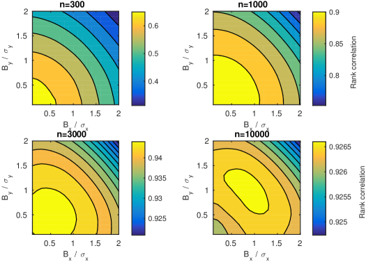
Figure 4: Illustration of the effect of projecting the outliers in linear regression, for different sample sizes $n$ with 10-dimensional synthetic data, evaluated by Spearman’s rank correlation between the predicted and true values. The $x$ and $y$ axes denote the projection thresholds as a function of standard deviations of data. Top right corner illustrates projection threshold at 2 standard deviations, no outlier projection would be further to top right. Higher values (yellow) are better. The result illustrates a clear benefit from the projection for moderate sample sizes, but the benefit decreases for really large sample sizes.

The privacy budget proportions $p_{1},p_{2},p_{3}$ and projection thresholds $B_{x}$, $B_{y}$ are important parameters for good model performance. As illustrated in Fig. 4, the projection thresholds depend strongly on the size of the data set. We propose finding the optimal parameter values on an auxiliary synthetic data set of the same size, which was found to be effective in our case. We generate the auxiliary data set of $n$ samples using a generative model similar to the one specified in Eq. (4.1):

$$x_{i} \sim N(0,I_{d})$$

$$y_{i}|x_{i} \sim N(x_{i}^{T}\beta,\lambda)$$

$$\beta \sim N(0,\lambda_{0}I),$$ (10)

where $d$ is the dimension.

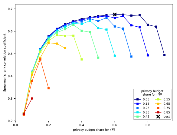
Figure 5: Optimal privacy budget split between sufficient statistics. Accuracy on a synthetic data set improves as a bigger proportion of the fixed privacy budget is assigned for $n\macc@depth\char 1\relax\frozen@everymath{\macc@group}\macc@set@skewchar\macc@nested@a 111{x}$. The best performance is achieved by assigning term $n\macc@depth\char 1\relax\frozen@everymath{\macc@group}\macc@set@skewchar\macc@nested@a 111{y}$ the smallest proportion 5%, term $n\macc@depth\char 1\relax\frozen@everymath{\macc@group}\macc@set@skewchar\macc@nested@a 111{x}$ a large 60% proportion, and term $n\macc@depth\char 1\relax\frozen@everymath{\macc@group}\macc@set@skewchar\macc@nested@a 111{x}$ the remaining 35% proportion of the privacy budget.

First we find the optimal budget split $p_{1},p_{2},p_{3}$. For all possible combinations of $(p_{1},p_{2},p_{3})\in\{0.05,0.1,\ldots,0.90\}^{3}$, where $p_{1}+p_{2}+p_{3}=1$, we project the data using clipping thresholds for the current split, and we perturb the sufficient statistics according to the current budget split. We compute the prediction as in Eq. (8) using samples drawn from the variational distribution fitted with ADVI and compute the error with respect to the original values. The error measure we use is Spearman’s rank correlation between the original and predicted values. The split $(p_{1},p_{2},p_{3})$ which gives the minimum error is used in all test settings. As illustrated in Fig. 5, in our experiments the optimal split gives the largest proportion of the privacy budget to the term $n\macc@depth\char 1\relax\frozen@everymath{\macc@group}\macc@set@skewchar\macc@nested@a 111{x}$ (60%), the second largest proportion to the term $n\macc@depth\char 1\relax\frozen@everymath{\macc@group}\macc@set@skewchar\macc@nested@a 111{x}$ (35%), and the smallest possible proportion to the term $n\macc@depth\char 1\relax\frozen@everymath{\macc@group}\macc@set@skewchar\macc@nested@a 111{y}$ (5%).

We parameterise the projection thresholds as a function of the data standard deviation as

$$B_{x}=\omega_{x}\sigma_{x},\quad B_{y}=\omega_{y}\sigma_{y}$$ (11)

$$\omega_{x},\omega_{y}\in\{0.1\omega\}_{\omega=1}^{20},$$ (12)

where the $\sigma_{x}$ and $\sigma_{y}$ are the standard deviations of $x$ (considering all dimensions) and $y$, respectively. With all 400 pairs of $(B_{x},B_{y})$ as specified above, we apply the outlier projection method of Eq. (4.3). We perturb the sufficient statistics according to the chosen optimal privacy budget split and fit the model as in Eq. (3),4 using the projected values and then compute the error with respect to the original values. The pair of $(\omega_{x},\omega_{y})$ which gives the minimum error is used to define the $(B_{x},B_{y})$ for the real data as in Eq. (11). As the error we used Spearman’s rank correlation between original $y_{1:n}$ and predicted $\bar{y}_{1:n}$ based on the model learnt with projected values.

4.4 Data and pre-processing

We used the gene expression and drug sensitivity data from the Genomics of Drug Sensitivity in Cancer (GDSC) project [27, 11] (release 6.1, March 2017, http://www.cancerrxgene.org) consisting of 265 drugs and a panel of 985 human cancer cell lines. The dimensionality of the RMA-normalised gene expression data was reduced from $d=17490$ down to 64 based on prior knowledge about genes that are frequently mutated in cancer, provided by the GDSC project at http://www.cancerrxgene.org/translation/Gene. We further ordered the genes based on their mutation counts as reported at http://cancer.sanger.ac.uk/cosmic/curation. Drug responses were quantified by log-transformed IC50 values (the drug concentration yielding 50% response) from the dose response data measured at 9 different concentrations. The mean was first removed from each gene, $x_{ij}:=x_{ij}-\mathrm{mean}(x_{i:n,j})$, and each data point was normalised to have L2-norm $\|x_{i}\|_{2}=1$, which focuses the analysis on relative expression of the selected genes, and equalises the contribution of each data point. The mean was removed from drug sensitivities, $y_{i}:=y_{i}-\mathrm{mean}(y_{1:n})$. Data with missing drug responses were ignored, making the number of cell lines different across different drugs.

4.5 Experimental setup

We carried out a 50-fold Monte Carlo cross-validation process for different splits of the data set into train and test using different random seeds. For each repeat, we randomly split the 985 cell lines to 100 for testing and the rest for training. We further randomly partitioned the training set to 30 non-private cell lines and used the rest as the private data set. In the experiments, we tested non-private data sizes from 0 to 30, and private data sizes from 100 to 800. The hyperparameters for the Gamma priors of precision parameters $\lambda,\lambda_{0}$ in Eq. (4.1) were set to $a=b=a_{0}=b_{0}=2$. The Gamma(2,2) distribution has mean 1 and variance 1/2 and defines a realistic distribution over sensible values of precision parameters which should be larger than zero. We implemented the model and carried out the inference with the PyMC3 Python module [20]. Using ADVI, we fitted a normal distribution with uncorrelated variables to the posterior distribution. We computed the drug response predictions using $m=5000$ samples from the fitted variational distribution. We used ADVI because it gives similar results as Hamiltonian Monte Carlo sampling but significantly faster. The optimal privacy budget split was based on prediction performance averaged over five auxiliary data sets of 500 synthetic samples (approximately half of the GDSC data set size) and five generated noise samples, and for each split, the optimal projection thresholds were chosen similarly based on average performance over five auxiliary data sets and five noise samples. The prediction for each split was computed using $m=5000$ samples drawn from the variational distribution fitted with ADVI. The final optimal projection thresholds for each test case were chosen using the optimal budget split and based on average prediction performance over 20 auxiliary data sets and 20 noise samples. All auxiliary data sets were generated by fixing the precision parameter values to the prior means, $\lambda=\lambda_{0}=1$. The prediction for each pair of projection thresholds was also computed using fixed precision parameters as in Eq. (3) and Eq. (4), as generating samples from the fitted variational distribution for all test cases would have been infeasible in practice.

4.6 Alternative methods used in comparisons

We compared five models: (i) linear regression (LR) as defined in Eq. (4.1), (ii) robust private LR is the proposed method, and (iii) private LR is the proposed method without projection of the outliers, (iv) output perturbed LR [26], and (v) functional mechanism LR [28]. Output perturbed LR learns parameters $\beta$ using the same LR model in Eq. (4.1), but instead of statistics the parameters are perturbed, in a data-independent manner. Our implementation of output perturbed LR makes use of minConf optimisation package [21]. For functional mechanism LR we used the code publicly available at https://sourceforge.net/projects/functionalmecha/.

4.7 Alternative interpretation: transformed linear regression

The outlier projection mechanism can also be interpreted to produce a transformed linear regression problem,

$$\phi_{y}(y_{i})|x_{i}\sim N(\phi_{x}(x_{i})^{T}\beta,\lambda),$$ (13)

where the functions $\phi_{y}()$ and $\phi_{x}()$ implementing the outlier projection can be defined as

$$\phi_{y}(y_{i}) =\max(-B_{y},\min(B_{y},y_{i}))$$ (14)

$$\phi_{x}(x_{i}) =\max(-B_{x},\min(B_{x},x_{i})).$$ (15)

The normalisation of data can also be included as a transformation. This interpretation makes explicit the flexibility in designing the transformations: the differential privacy guarantees will remain valid as long as the transformations obey the bounds

$$\phi_{y}(y_{i})\in[-B_{y},B_{y}],\quad\phi_{x}(x_{i})\in[-B_{x},B_{x}].$$ (16)

Acknowledgements

We would like to thank Muhammad Ammad-ud-din for assistance in data processing and Otte Heinävaara for assistance in the theoretical analysis. We acknowledge the computational resources provided by the Aalto Science-IT project. This work was funded by the Academy of Finland (Centre of Excellence COIN; and grants 283193 (S.K. and M.D), 294238 and 292334 (S.K.), 278300 (A.H. and O.D.), 259440 and 283107 (A.H.)).

Supplementary Information

Appendix A Theoretical background

We argue that effective differentially private predictive modelling methods can be developed by a combination of:

1. An asymptotically efficiently private mechanism for which the effect of the noise added to guarantee privacy vanishes as the number of samples increases; and

2. A way to limit the amount of private information to be shared. This yields better performance on finite data as less noise needs to be added for equivalent privacy. This can be achieved through a combination of two things:

   1. An approach to decrease the dimensionality of the data prior to the application of the private algorithm; and

   2. A method to focus the privacy guarantees to relevant variation in data.

Criterion i can be formally stated through additional loss in accuracy or utility of the estimates because of privacy. Our main asymptotic result is that the optimal convergence rate of a differentially private mechanism to a Bayesian estimate is $\mathcal{O}(1/n)$, which can be reached by our proposed mechanism.

Criterion ii is non-asymptotic and thus more difficult to address theoretically. It manifests itself in the constants in the convergence rates as well as empirical findings on the effect of dimensionality reduction and projecting outliers to tighter bounds as discussed in the main text and in Fig. 4.

A.1 Definition of asymptotic efficiency

We begin by formalisation of the theory behind Criterion i.

Definition 1.

A differentially private mechanism $\mathcal{M}$ is asymptotically consistent with respect to an estimated parameter $\theta$ if the private estimates $\hat{\theta}_{\mathcal{M}}$ given a data set $\mathcal{D}$ converge in probability to the corresponding non-private estimates $\hat{\theta}_{NP}$ as the number of samples, $n=|\mathcal{D}|$, grows without bound, i.e., if for any $\alpha>0$,

$$\lim\limits_{n\rightarrow\infty}\mathrm{Pr}\{\|\hat{\theta}_{\mathcal{M}}-\hat{\theta}_{NP}\|>\alpha\}=0.$$

Definition 2.

A differentially private mechanism $\mathcal{M}$ is asymptotically efficiently private with respect to an estimated parameter $\theta$, if the mechanism is asymptotically consistent and the private estimates $\hat{\theta}_{\mathcal{M}}$ converge to the corresponding non-private estimates $\hat{\theta}_{NP}$ at the rate $\mathcal{O}(1/n)$, i.e., if for any $\alpha>0$ there exist constants $C,N$ such that

$$\mathrm{Pr}\{\|\hat{\theta}_{\mathcal{M}}-\hat{\theta}_{NP}\|>C/n\}<\alpha$$

for all $n\geq N$.

The term asymptotically efficiently private in the above definition is justified by the following theorem, which shows that the rate $\mathcal{O}(1/n)$ is optimal for estimating expectation parameters of exponential family distributions. As it seems unlikely that better rates could be obtained for more difficult problems, we conjecture that this rate cannot be beaten for Bayesian estimates in general.

Theorem 1.

The private estimates $\hat{\theta}_{\mathcal{M}}$ of an exponential family posterior expectation parameter $\theta$, generated by a differentially private mechanism $\mathcal{M}$ that achieves $\epsilon$-differential privacy for any $\epsilon>0$, cannot converge to the corresponding non-private estimates $\hat{\theta}_{NP}$ at a rate faster than $1/n$. This is, assuming $\mathcal{M}$ is $\epsilon$-differentially private, there exists no function $f(n)$ such that $\lim\sup nf(n)=0$ and for all $\alpha>0$, there exists a constant $N$ such that

$$\mathrm{Pr}\{\|\hat{\theta}_{\mathcal{M}}-\hat{\theta}_{NP}\|>f(n)\}<\alpha$$

for all $n\geq N$.

Proof.

The non-private estimate of an expectation parameter of an exponential family is [5]

$$\hat{\theta}_{NP}|x_{1},\dots,x_{n}=\frac{n_{0}x_{0}+\sum_{i=1}^{n}x_{i}}{n_{0}+n}.$$ (17)

The difference of the estimates from two neighbouring data sets differing by one element is

$$(\hat{\theta}_{NP}|\mathcal{D})-(\hat{\theta}_{NP}|\mathcal{D}^{\prime})=\frac{x-y}{n_{0}+n},$$ (18)

where $x$ and $y$ are the corresponding mismatched elements. Let $\Delta=\max(\|x-y\|)$, and let $\mathcal{D}$ and $\mathcal{D}^{\prime}$ be neighbouring data sets including these maximally different elements.

Let us assume that there exists a function $f(n)$ such that $\lim\sup nf(n)=0$ and for all $\alpha>0$ there exists a constant $N$ such that

$$\mathrm{Pr}\{\|\hat{\theta}_{\mathcal{M}}-\hat{\theta}_{NP}\|>f(n)\}<\alpha$$

for all $n\geq N$.

Fix $\alpha>0$ and choose $M\geq\max(N,n_{0})$ such that $f(n)\leq\Delta/4n$ for all $n\geq M$. This implies that

$$\|(\hat{\theta}_{NP}|\mathcal{D})-(\hat{\theta}_{NP}|\mathcal{D}^{\prime})\|=\frac{\Delta}{n_{0}+n}\geq\frac{\Delta}{2n}\geq 2f(n).$$ (19)

Let us define the region $C_{\mathcal{D}}=\{t\;|\;\|(\hat{\theta}_{NP}|\mathcal{D})-t\|<f(n)\}.$ Based on our assumptions we have

$$\mathrm{Pr}(\hat{\theta}_{\mathcal{M}}|\mathcal{D}\in C_{\mathcal{D}}) >1-\alpha$$ (20)

$$\mathrm{Pr}(\hat{\theta}_{\mathcal{M}}|\mathcal{D}^{\prime}\in C_{\mathcal{D}}) <\alpha$$ (21)

which implies that

$$\frac{\mathrm{Pr}(\hat{\theta}_{\mathcal{M}}|\mathcal{D}\in C_{\mathcal{D}})}{\mathrm{Pr}(\hat{\theta}_{\mathcal{M}}|\mathcal{D}^{\prime}\in C_{\mathcal{D}})}>\frac{1-\alpha}{\alpha}$$ (22)

which means that $\mathcal{M}$ cannot be differentially private with $\epsilon<\log\left((1-\alpha)/\alpha\right)\rightarrow\infty$ as $\alpha\rightarrow 0$. ∎

A.2 Different utility functions

Definition 3.

Let $\mathcal{U}(\hat{\theta}_{NP}(\mathcal{D}))$ measure the utility of the non-private model $\hat{\theta}_{NP}$ estimated from data set $\mathcal{D}$ and let $\mathcal{U}(\hat{\theta}_{\mathcal{M}}(\mathcal{D}))$ measure the corresponding utility of the private model $\hat{\theta}_{\mathcal{M}}$ obtained using differentially private mechanism $\mathcal{M}$. The mechanism $\mathcal{M}$ is asymptotically consistent with respect to a bounded utility $\mathcal{U}$ if the random variables $\mathcal{U}(\hat{\theta}_{\mathcal{M}}(\mathcal{D}))$ converge in probability to $\mathcal{U}(\hat{\theta}_{NP}(\mathcal{D}))$ as the number of samples, $n=|\mathcal{D}|$, grows without bound, i.e., if for any $\alpha>0$,

$$\lim\limits_{n\rightarrow\infty}\mathrm{Pr}\{|\mathcal{U}(\hat{\theta}_{\mathcal{M}}(\mathcal{D}))-\mathcal{U}(\hat{\theta}_{NP}(\mathcal{D}))|>\alpha\}=0.$$

Theorem 2.

A differentially private mechanism $\mathcal{M}$ that is asymptotically consistent with respect to a set of parameters is asymptotically consistent with respect to any continuous utility that only depends on those parameters.

Proof.

If $\hat{\theta}_{\mathcal{M}}$ converges in probability to $\hat{\theta}_{NP}$ then by the continuous mapping theorem the value of $\mathcal{U}(\hat{\theta}_{\mathcal{M}})$ will converge in probability to $\mathcal{U}(\hat{\theta}_{NP})$. ∎

A.3 Example: Gaussian mean

Theorem 3.

Differentially private inference of the mean of a Gaussian variable, with Laplace mechanism to perturb the sufficient statistics, is asymptotically consistent with respect to the posterior mean.

Proof.

Let us consider the model

$$x_{i} \sim N(\mu,\Lambda)$$

$$\mu \sim N(\mu_{0},\Lambda_{0})$$

with $\mu$ as the unknown parameter and $\Lambda$ and $\Lambda_{0}$ denoting the fixed prior precision matrices of the noise and the mean, respectively. We assume $||x_{i}||_{1}\leq B$ and enforce this by projecting the larger elements to satisfy this bound.

Let the observed data set be $\mathcal{D}=\{x_{i}\}_{i=1}^{n}$ with sufficient statistic $n\bar{x}=\sum_{i=1}^{n}x_{i}$.

The non-private posterior mean is

$$\mu_{NP}=(\Lambda_{0}+n\Lambda)^{-1}(\Lambda n\bar{x}+\Lambda_{0}\mu_{0}).$$

The corresponding private posterior mean is obtained by replacing $n\bar{x}$ with the perturbed version $n\bar{x}^{\prime}=n\bar{x}+\delta$, where $\delta=(\delta_{1},\dots,\delta_{d})^{T}\in\mathbb{R}^{d}$ with $\delta_{j}\sim\mathrm{Laplace}(0,\frac{2Bd}{\epsilon})$ and $d=\dim(x_{i})$, yielding

$$\mu_{DP}=(\Lambda_{0}+n\Lambda)^{-1}(\Lambda(n\bar{x}+\delta)+\Lambda_{0}\mu_{0}).$$

The difference of the private and non-private means is

$$\|\mu_{DP}-\mu_{NP}\|_{1} =\|(\Lambda_{0}+n\Lambda)^{-1}(\Lambda\delta)\|_{1}$$

$$=\|(\Lambda^{-1}\Lambda_{0}+n\cdot I)^{-1}\delta\|_{1}\leq\frac{c}{n}\|\delta\|_{1},$$

which is valid for all $c>1$ for large enough $n$. This implies that

$$\mathrm{Pr}\{\|\mu_{DP}-\mu_{NP}\|_{1}\geq\alpha\}\leq\mathrm{Pr}\left\{\frac{c}{n}\|\delta\|_{1}\geq\alpha\right\}\rightarrow 0$$

as $n\rightarrow\infty$ for all $\alpha>0$. ∎

Theorem 4.

Differentially private inference of the mean of a Gaussian variable with Laplace mechanism to perturb the input data set (naive input perturbation) is not asymptotically consistent with respect to the posterior mean.

Proof.

The mechanism is almost the same as in Theorem 3, but we now have $n\bar{x}^{\prime}=n\bar{x}+\sum_{i=1}^{n}\delta_{i})$ where $\delta_{i}=(\delta_{i1},\dots,\delta_{id})^{T}\in\mathbb{R}^{d}$ with $\delta_{ij}\sim\mathrm{Laplace}(0,\frac{2Bd}{\epsilon})$. Similar computation as above yields

$$\|\mu_{DP}-\mu_{NP}\|_{1} =\left\|(\Lambda_{0}+n\Lambda)^{-1}(\Lambda\sum_{i=1}^{n}\delta_{i})\right\|_{1}$$

$$=\left\|(\frac{1}{n}\Lambda^{-1}\Lambda_{0}+I)^{-1}\frac{1}{n}\sum_{i=1}^{n}\delta_{i}\right\|_{1}\geq\frac{1}{2}\left\|\frac{1}{n}\sum_{i=1}^{n}\delta_{i}\right\|_{1}$$

for sufficiently large $n$. By the central limit theorem the distribution of $\frac{1}{n}\sum_{i=1}^{n}\delta_{i}$ converges to a Gaussian with non-zero variance. Hence $\mu_{DP}$ does not converge to $\mu_{NP}$ for large $n$ and the method is not asymptotically consistent. ∎

A.3.1 Asymptotic efficiency

Theorem 5.

$\epsilon$-differentially private estimate of the mean of a $d$-dimensional Gaussian variable $x$ bounded by $\|x_{i}\|_{1}\leq B$ in which the Laplace mechanism is used to perturb the sufficient statistics, is asymptotically efficiently private.

Proof.

In the proof of Theorem 3 we showed that

$$\|\mu_{DP}-\mu_{NP}\|_{1}\leq\frac{c}{n}\|\delta\|_{1},$$

where $\delta=(\delta_{1},\dots,\delta_{d})^{T}\in\mathbb{R}^{D}$ with $\delta_{j}\sim\mathrm{Laplace}\left(0,\frac{2Bd}{\epsilon}\right)$.

Because $\delta_{j}$ is Laplace, $|\delta_{j}|$ is exponential with

$$|\delta_{j}|\sim\mathrm{Exponential}\left(\frac{\epsilon}{2Bd}\right)$$

and

$$\|\delta\|_{1}=\sum_{j=1}^{d}|\delta_{j}|\sim\mathrm{Gamma}\left(d,\frac{\epsilon}{2Bd}\right).$$

Given $\alpha>0$ we can choose $C>cF^{-1}(1-\alpha;d,\epsilon/2Bd)$, where $F^{-1}(x;a,b)$ is the inverse cumulative distribution function of the Gamma distribution with shape $a$ and rate $b$, to ensure that

$$\mathrm{Pr}\left\{\|\mu_{DP}-\mu_{NP}\|_{1}>\frac{C}{n}\right\}\leq\mathrm{Pr}\left\{\frac{1}{n}\|\delta\|_{1}>\frac{C}{n}\right\}=\mathrm{Pr}\{\|\delta\|_{1}>C\}<\alpha.$$ (23)

∎

A.3.2 Convergence rate

We can further study the probability of making an error of at least a given magnitude as

$$\mathrm{Pr}\{\|\mu_{DP}-\mu_{NP}\|_{1}\geq\phi\} \leq\mathrm{Pr}\left\{\frac{c}{n}\|\delta\|_{1}\geq\phi\right\}$$

$$=\mathrm{Pr}\left\{\mathrm{Gamma}\left(d,\frac{n\epsilon}{2Bcd}\right)\geq\phi\right\}$$

$$=1-F\left(\phi;d,\frac{n\epsilon}{2Bcd}\right)=1-\frac{\gamma(d,\frac{n\phi\epsilon}{2Bcd})}{\Gamma(d)},$$ (24)

where $F(x;a,b)$ is the cumulative distribution function of the Gamma distribution with shape $a$ and rate $b$.

The formula in Eq. (24) unfortunately has no simple closed form expression. The result shows, however, that the $n$ required to reach a certain level of performance is linear in $B$ and $\frac{1}{\epsilon}$. The dependence on $d$ is complicated, but it is in general super-linear as suggested by the mean of the gamma distribution in Eq. (24), $\frac{2Bd^{2}}{n\epsilon}$.

A.4 Example: Zhang et al., AAAI 2016, (arxiv:1512.06992)

In their paper Zhang et al. derive utility bounds for a number of mechanisms. The bounds are clearly insufficient to demonstrate the asymptotic efficiency of the corresponding methods. For Laplace mechanism applied to Bayesian network inference, their bound on excess KL-divergence as a function of the data set size $n$ is

$$\mathcal{O}(mn\ln n)\left[1-\exp\left(-\frac{n\epsilon}{2|\mathcal{I}|}\right)\right]+\sqrt{-\mathcal{O}(mn\ln n)\ln\delta}.$$

Appendix B Differentially private linear regression

Let us next consider the linear regression model with fixed noise $\Lambda$,

$$y_{i}|x_{i} \sim N(x_{i}^{T}\beta,\Lambda)$$

$$\beta \sim N(\beta_{0},\Lambda_{0}),$$

with $\beta$ as the unknown parameter and $\Lambda$ and $\Lambda_{0}$ denoting the precision matrices of the corresponding distributions.

Let the observed data set be $\mathcal{D}=\{(x_{i},y_{i})\}_{i=1}^{n}$ with sufficient statistics $n\macc@depth\char 1\relax\frozen@everymath{\macc@group}\macc@set@skewchar\macc@nested@a 111{x}=\sum_{i=1}^{n}x_{i}x_{i}^{T}$ and $n\macc@depth\char 1\relax\frozen@everymath{\macc@group}\macc@set@skewchar\macc@nested@a 111{x}=\sum_{i=1}^{n}x_{i}y_{i}$.

The non-private posterior precision of $\beta$ is

$$\Lambda_{NP}=\Lambda_{0}+\Lambda n\macc@depth\char 1\relax\frozen@everymath{\macc@group}\macc@set@skewchar\macc@nested@a 111{x}$$

and the corresponding posterior mean is

$$\mu_{NP}=\Lambda_{NP}^{-1}(\Lambda n\macc@depth\char 1\relax\frozen@everymath{\macc@group}\macc@set@skewchar\macc@nested@a 111{x}+\Lambda_{0}\beta_{0}).$$ (25)

The corresponding private posterior precision is obtained by replacing $n\macc@depth\char 1\relax\frozen@everymath{\macc@group}\macc@set@skewchar\macc@nested@a 111{x}$ with the perturbed version $n\macc@depth\char 1\relax\frozen@everymath{\macc@group}\macc@set@skewchar\macc@nested@a 111{x}^{\prime}=n\macc@depth\char 1\relax\frozen@everymath{\macc@group}\macc@set@skewchar\macc@nested@a 111{x}+\Delta$, where $\Delta$ follows the Laplace distribution according to the Laplace mechanism, yielding

$$\Lambda_{DP}=\Lambda_{0}+\Lambda(n\macc@depth\char 1\relax\frozen@everymath{\macc@group}\macc@set@skewchar\macc@nested@a 111{x}+\Delta).$$

Similarly using $n\macc@depth\char 1\relax\frozen@everymath{\macc@group}\macc@set@skewchar\macc@nested@a 111{x}^{\prime}=n\macc@depth\char 1\relax\frozen@everymath{\macc@group}\macc@set@skewchar\macc@nested@a 111{x}+\delta$ with $\delta$ following the Laplace mechanism we obtain

$$\mu_{DP}=\Lambda_{DP}^{-1}(\Lambda(n\macc@depth\char 1\relax\frozen@everymath{\macc@group}\macc@set@skewchar\macc@nested@a 111{x}+\delta)+\Lambda_{0}\beta_{0}).$$ (26)

As presented in Methods, a more robust alternative is to assign prior distributions to the precision parameters and then sample the posterior. This requires using the three sufficient statistics $n\macc@depth\char 1\relax\frozen@everymath{\macc@group}\macc@set@skewchar\macc@nested@a 111{x}$, $n\macc@depth\char 1\relax\frozen@everymath{\macc@group}\macc@set@skewchar\macc@nested@a 111{x}$, and $n\macc@depth\char 1\relax\frozen@everymath{\macc@group}\macc@set@skewchar\macc@nested@a 111{y}$ that are perturbed with suitable noise. The mechanism is presented in detail in Algorithm 1 and proven to guarantee differential privacy in Theorem 6. For theoretical analysis, we study the model with fixed precision parameters and an even privacy budget split between the two needed sufficient statistics. In Algorithm 1 and Theorem 6, this corresponds to setting $p_{1}=p_{2}=0.5$ and leaving out the unnecessary term $S_{yy}$.

B.1 The detailed mechanism

Algorithm 1 Differentially private statistics release

$p_{1}+p_{2}+p_{3}=1$

function DiffPriSS($X$, $Y$, $\epsilon$, $B_{x}$, $B_{y}$)

     $n=|Y|$, $d=\mathrm{dim}(X)$

     $(C,D)=\textsc{project}(X,Y,B_{x},B_{y})$

     for $i\in\{1,\dots,n\}$ do

         for $j\in\{i,\dots,n\}$ do

              $P_{ij}=P_{ji}\sim\mathrm{Laplace}\left(0,\frac{d(d+1)B_{x}^{2}}{p_{1}\epsilon}\right)$

         end for

     end for

     for $i\in\mathbb{I}$ do

         $Q_{i}\sim\mathrm{Laplace}\left(0,\frac{2dB_{x}B_{y}}{p_{2}\epsilon}\right)$

     end for

     $R\sim\mathrm{Laplace}\left(0,\frac{B_{y}^{2}}{p_{3}\epsilon}\right)$

     $S_{xx}=CC^{\prime}+P$

     $S_{xy}=CD+Q$

     $S_{yy}=DD^{\prime}+R$

end function

function Project($X$, $Y$, $B_{x}$, $B_{y}$)

     for $j=1$ to $n$ do

         for $i=1$ to $d$ do

              $C_{ij}=\max(-B_{x},\min(B_{x},X_{ij}))$

         end for

         $D_{j}=\max(-B_{y},\min(B_{y},Y_{j}))$

     end for

end function

The function project in Algorithm 1 projects the data points into a useful space and computes the sufficient statistics.

Theorem 6.

Algorithm DiffPriSS in Algorithm 1 is $\epsilon$-differentially private.

Proof.

(i) $S_{xx}=CC^{\prime}+P$ is $p_{1}\epsilon$-differentially private.

$S_{xx}$ is a symmetric $d\times d$ matrix with $\frac{d(d+1)}{2}$ degrees of freedom. After project $|C|_{\infty}\leq B_{x}$ and the sensitivity of each element $\Delta(S_{xx})_{ij}=\sup|c_{i}c_{j}-c_{i}^{\prime}c_{j}^{\prime}|\leq 2B_{x}^{2}$. Adding Laplace distributed noise to $(S_{xx})_{ij}$ with $b=\frac{d(d+1)B_{x}^{2}}{p_{1}\epsilon}$ yields an $\epsilon^{\prime}$-DP mechanism with $\epsilon^{\prime}=\frac{2p_{1}\epsilon}{d(d+1)}$. Using basic composition [8] over the $\frac{d(d+1)}{2}$ independent dimensions shows that $S_{xx}=CC^{\prime}+P$ is $p_{1}\epsilon$-differentially private.

(ii) $CD$ is a $d\times 1$ vector where $d$ is the cardinality of $\mathbb{I}$ and each element of $CD$ is computed as follows:

$$\forall i\in\mathbb{I},\;\;CD_{i}=\sum_{j=1}^{n}C_{ij}D_{j},$$ (27)

where $|C_{ij}|\leq B_{x}$ and $|D_{j}|\leq B_{y}$, and thus the sensitivity of $CD$ is $2dB_{x}B_{y}$. Thus, $S_{xy}=CD+Q$ is $p_{2}\epsilon$-differentially private.

(iii) $DD^{\prime}$ is a scalar computed as

$$DD^{\prime}=\sum_{j=1}^{n}D_{j}^{2},$$

where $|D_{j}|\leq B_{y}$, and thus the sensitivity of $DD^{\prime}$ is $B_{y}^{2}$. Thus, $S_{yy}=DD^{\prime}+R$ is $p_{3}\epsilon$-differentially private.

Therefore, releasing $S_{xx}$, $S_{xy}$, and $S_{yy}$ together by DiffPriSS is $\epsilon$-differentially private. ∎

B.2 Asymptotic consistency and efficiency

Theorem 7.

Differentially private inference of the posterior mean of the weights of linear regression with Laplace mechanism to perturb the sufficient statistics is asymptotically consistent with respect to the posterior mean.

Proof.

Using Eqs. (25)–(26) we can evaluate

$$\left\|\mu_{DP}-\mu_{NP}\right\|_{1} =\left\|\Lambda_{DP}^{-1}(\Lambda(n\macc@depth\char 1\relax\frozen@everymath{\macc@group}\macc@set@skewchar\macc@nested@a 111{x}+\delta)+\Lambda_{0}\beta_{0})-\Lambda_{NP}^{-1}(\Lambda n\macc@depth\char 1\relax\frozen@everymath{\macc@group}\macc@set@skewchar\macc@nested@a 111{x}+\Lambda_{0}\beta_{0})\right\|_{1}$$

$$\leq\left\|\Lambda_{DP}^{-1}(\Lambda(n\macc@depth\char 1\relax\frozen@everymath{\macc@group}\macc@set@skewchar\macc@nested@a 111{x}+\delta)+\Lambda_{0}\beta_{0})-\Lambda_{DP}^{-1}(\Lambda n\macc@depth\char 1\relax\frozen@everymath{\macc@group}\macc@set@skewchar\macc@nested@a 111{x}+\Lambda_{0}\beta_{0})\right\|_{1}$$

$$\phantom{\leq}+\left\|\Lambda_{DP}^{-1}(\Lambda n\macc@depth\char 1\relax\frozen@everymath{\macc@group}\macc@set@skewchar\macc@nested@a 111{x}+\Lambda_{0}\beta_{0})-\Lambda_{NP}^{-1}(\Lambda n\macc@depth\char 1\relax\frozen@everymath{\macc@group}\macc@set@skewchar\macc@nested@a 111{x}+\Lambda_{0}\beta_{0})\right\|_{1}$$

$$=\left\|\Lambda_{DP}^{-1}\Lambda\delta\right\|_{1}+\left\|(\Lambda_{DP}^{-1}-\Lambda_{NP}^{-1})(\Lambda n\macc@depth\char 1\relax\frozen@everymath{\macc@group}\macc@set@skewchar\macc@nested@a 111{x}+\Lambda_{0}\beta_{0})\right\|_{1}$$

$$=\left\|(\Lambda_{0}+\Lambda(n\macc@depth\char 1\relax\frozen@everymath{\macc@group}\macc@set@skewchar\macc@nested@a 111{x}+\Delta))^{-1}\Lambda\delta\right\|_{1}$$

$$\phantom{=}+\big{\|}\big{[}(\Lambda_{0}+\Lambda(n\macc@depth\char 1\relax\frozen@everymath{\macc@group}\macc@set@skewchar\macc@nested@a 111{x}+\Delta))^{-1}$$

$$\phantom{=+\big{\|}\big{[}\;}-(\Lambda_{0}+\Lambda(n\macc@depth\char 1\relax\frozen@everymath{\macc@group}\macc@set@skewchar\macc@nested@a 111{x}))^{-1}\big{]}(\Lambda n\macc@depth\char 1\relax\frozen@everymath{\macc@group}\macc@set@skewchar\macc@nested@a 111{x}+\Lambda_{0}\beta_{0})\big{\|}_{1}$$

$$=\left\|(\Lambda_{0}+\Lambda(n\macc@depth\char 1\relax\frozen@everymath{\macc@group}\macc@set@skewchar\macc@nested@a 111{x}+\Delta))^{-1}\Lambda\delta\right\|_{1}$$

$$\phantom{=}+\bigg{\|}\bigg{[}\left(\frac{1}{n}\Lambda_{0}+\Lambda\left(\macc@depth\char 1\relax\frozen@everymath{\macc@group}\macc@set@skewchar\macc@nested@a 111{x}+\frac{1}{n}\Delta\right)\right)^{-1}$$

$$\phantom{=+\bigg{\|}\bigg{[}\;}-\left(\frac{1}{n}\Lambda_{0}+\Lambda\macc@depth\char 1\relax\frozen@everymath{\macc@group}\macc@set@skewchar\macc@nested@a 111{x}\right)^{-1}\bigg{]}\left(\Lambda\macc@depth\char 1\relax\frozen@everymath{\macc@group}\macc@set@skewchar\macc@nested@a 111{x}+\frac{1}{n}\Lambda_{0}\beta_{0}\right)\bigg{\|}_{1}.$$

Assuming $\macc@depth\char 1\relax\frozen@everymath{\macc@group}\macc@set@skewchar\macc@nested@a 111{x}>0$, the first term clearly approaches 0 as $n\rightarrow\infty$. For the second term, as $n\rightarrow\infty$, $(\frac{1}{n}\Lambda_{0}+\Lambda(\macc@depth\char 1\relax\frozen@everymath{\macc@group}\macc@set@skewchar\macc@nested@a 111{x}+\frac{1}{n}\Delta))^{-1}\rightarrow(\frac{1}{n}\Lambda_{0}+\Lambda\macc@depth\char 1\relax\frozen@everymath{\macc@group}\macc@set@skewchar\macc@nested@a 111{x})^{-1}$ and as $(\Lambda\macc@depth\char 1\relax\frozen@everymath{\macc@group}\macc@set@skewchar\macc@nested@a 111{x}+\frac{1}{n}\Lambda_{0}\beta_{0})$ is bounded, the second term also approaches 0 as $n\rightarrow\infty$. This shows that $\mu_{DP}$ converges in probability to $\mu_{NP}$. ∎

Theorem 8.

$\epsilon$-differentially private inference of the posterior mean of the weights of linear regression with the Laplace mechanism of Algorithm 1 to perturb the sufficient statistics is asymptotically efficiently private.

Proof.

From the proof of Theorem 7 we have

$$\left\|\mu_{DP}-\mu_{NP}\right\|_{1}\leq\left\|(\Lambda_{0}+\Lambda(n\macc@depth\char 1\relax\frozen@everymath{\macc@group}\macc@set@skewchar\macc@nested@a 111{x}+\Delta))^{-1}\Lambda\delta\right\|_{1}\\ +\left\|\left[\left(\frac{1}{n}\Lambda_{0}+\Lambda\left(\macc@depth\char 1\relax\frozen@everymath{\macc@group}\macc@set@skewchar\macc@nested@a 111{x}+\frac{1}{n}\Delta\right)\right)^{-1}-\left(\frac{1}{n}\Lambda_{0}+\Lambda\macc@depth\char 1\relax\frozen@everymath{\macc@group}\macc@set@skewchar\macc@nested@a 111{x}\right)^{-1}\right]\left(\Lambda\macc@depth\char 1\relax\frozen@everymath{\macc@group}\macc@set@skewchar\macc@nested@a 111{x}+\frac{1}{n}\Lambda_{0}\beta_{0}\right)\right\|_{1}.$$ (28)

The first term can be bounded easily as

$$\left\|(\Lambda_{0}+\Lambda(n\macc@depth\char 1\relax\frozen@everymath{\macc@group}\macc@set@skewchar\macc@nested@a 111{x}+\Delta))^{-1}\Lambda\delta\right\|_{1} =\left\|(\Lambda^{-1}\Lambda_{0}+\Delta+n\macc@depth\char 1\relax\frozen@everymath{\macc@group}\macc@set@skewchar\macc@nested@a 111{x})^{-1}\delta\right\|_{1}$$

$$\leq\left\|(\Lambda^{-1}\Lambda_{0}+\Delta+n\macc@depth\char 1\relax\frozen@everymath{\macc@group}\macc@set@skewchar\macc@nested@a 111{x})^{-1}\right\|_{1}\|\delta\|_{1}$$

$$\leq\frac{c_{1}}{n}\left\|(\macc@depth\char 1\relax\frozen@everymath{\macc@group}\macc@set@skewchar\macc@nested@a 111{x})^{-1}\right\|_{1}\|\delta\|_{1}$$ (29)

where $c_{1}>1$. The bound is valid for any $c_{1}>1$ as $n$ gets large enough.

Similarly as in the proof of Theorem 5,

$$\|\delta\|_{1}\sim\mathrm{Gamma}\left(d,\frac{\epsilon}{4dB_{x}B_{y}}\right).$$ (30)

Given $\alpha>0$ we can choose similarly as in the proof of Theorem 5

$$C_{1}>c_{1}F^{-1}(1-\alpha/2;d,\epsilon/(4dB_{x}B_{y}))\left\|(\macc@depth\char 1\relax\frozen@everymath{\macc@group}\macc@set@skewchar\macc@nested@a 111{x})^{-1}\right\|_{1},$$

where $F^{-1}(x;\alpha,\beta)$ is the inverse distribution function of the Gamma distribution with shape $\alpha$ and rate $\beta$, to ensure that

$$\mathrm{Pr}\left\{\|(\Lambda_{0}+\Lambda(n\macc@depth\char 1\relax\frozen@everymath{\macc@group}\macc@set@skewchar\macc@nested@a 111{x}+\Delta))^{-1}\Lambda\delta\|_{1}>\frac{C_{1}}{n}\right\}<\frac{\alpha}{2}.$$ (31)

The second term can be bounded as

$$\left\|\left[\left(\frac{1}{n}\Lambda_{0}+\Lambda\left(\macc@depth\char 1\relax\frozen@everymath{\macc@group}\macc@set@skewchar\macc@nested@a 111{x}+\frac{1}{n}\Delta\right)\right)^{-1}-\left(\frac{1}{n}\Lambda_{0}+\Lambda\macc@depth\char 1\relax\frozen@everymath{\macc@group}\macc@set@skewchar\macc@nested@a 111{x}\right)^{-1}\right]\left(\Lambda\macc@depth\char 1\relax\frozen@everymath{\macc@group}\macc@set@skewchar\macc@nested@a 111{x}+\frac{1}{n}\Lambda_{0}\beta_{0}\right)\right\|_{1}\\ =\left\|\left[\left(\frac{1}{n}\Lambda^{-1}\Lambda_{0}+\macc@depth\char 1\relax\frozen@everymath{\macc@group}\macc@set@skewchar\macc@nested@a 111{x}+\frac{1}{n}\Delta\right)^{-1}-\left(\frac{1}{n}\Lambda^{-1}\Lambda_{0}+\macc@depth\char 1\relax\frozen@everymath{\macc@group}\macc@set@skewchar\macc@nested@a 111{x}\right)^{-1}\right]\left(\macc@depth\char 1\relax\frozen@everymath{\macc@group}\macc@set@skewchar\macc@nested@a 111{x}+\frac{1}{n}\Lambda^{-1}\Lambda_{0}\beta_{0}\right)\right\|_{1}\\ =\frac{1}{n}\left\|\left(\frac{1}{n}\Lambda^{-1}\Lambda_{0}+\macc@depth\char 1\relax\frozen@everymath{\macc@group}\macc@set@skewchar\macc@nested@a 111{x}+\frac{1}{n}\Delta\right)^{-1}\Delta\left(\frac{1}{n}\Lambda^{-1}\Lambda_{0}+\macc@depth\char 1\relax\frozen@everymath{\macc@group}\macc@set@skewchar\macc@nested@a 111{x}\right)^{-1}\left(\macc@depth\char 1\relax\frozen@everymath{\macc@group}\macc@set@skewchar\macc@nested@a 111{x}+\frac{1}{n}\Lambda^{-1}\Lambda_{0}\beta_{0}\right)\right\|_{1}\\ \leq\frac{1}{n}\left\|\left(\frac{1}{n}\Lambda^{-1}\Lambda_{0}+\macc@depth\char 1\relax\frozen@everymath{\macc@group}\macc@set@skewchar\macc@nested@a 111{x}+\frac{1}{n}\Delta\right)^{-1}\Delta\left(\frac{1}{n}\Lambda^{-1}\Lambda_{0}+\macc@depth\char 1\relax\frozen@everymath{\macc@group}\macc@set@skewchar\macc@nested@a 111{x}\right)^{-1}\right\|_{1}\left\|\macc@depth\char 1\relax\frozen@everymath{\macc@group}\macc@set@skewchar\macc@nested@a 111{x}+\frac{1}{n}\Lambda^{-1}\Lambda_{0}\beta_{0}\right\|_{1}\\ \leq\frac{1}{n}\left\|\left(\frac{1}{n}\Lambda^{-1}\Lambda_{0}+\macc@depth\char 1\relax\frozen@everymath{\macc@group}\macc@set@skewchar\macc@nested@a 111{x}+\frac{1}{n}\Delta\right)^{-1}\right\|_{1}\left\|\Delta\right\|_{1}\\ \left\|\left(\frac{1}{n}\Lambda^{-1}\Lambda_{0}+\macc@depth\char 1\relax\frozen@everymath{\macc@group}\macc@set@skewchar\macc@nested@a 111{x}\right)^{-1}\right\|_{1}\left\|\macc@depth\char 1\relax\frozen@everymath{\macc@group}\macc@set@skewchar\macc@nested@a 111{x}+\frac{1}{n}\Lambda^{-1}\Lambda_{0}\beta_{0}\right\|_{1}\\ \leq\frac{c_{2}}{n}\left\|\left(\macc@depth\char 1\relax\frozen@everymath{\macc@group}\macc@set@skewchar\macc@nested@a 111{x}\right)^{-1}\right\|_{1}\left\|\Delta\right\|_{1}\left\|\left(\macc@depth\char 1\relax\frozen@everymath{\macc@group}\macc@set@skewchar\macc@nested@a 111{x}\right)^{-1}\right\|_{1}\left\|\macc@depth\char 1\relax\frozen@everymath{\macc@group}\macc@set@skewchar\macc@nested@a 111{x}\right\|_{1}=:\frac{c_{2}}{n}\mathcal{B}_{2},$$

where similarly as in Eq. (29), the bound is valid for any $c_{2}>1$ as $n$ gets large enough. Here $\|\Delta\|_{1}$ is the $l_{1}$-norm of the matrix $\Delta$ that whose elements follow the Laplace distribution $\Delta_{ij}\sim\mathrm{Laplace}(0,\frac{2d(d+1)B_{x}^{2}}{\epsilon})$. We can bound it as

$$\|\Delta\|_{1}=\max_{i}\|\Delta_{:i}\|_{1},$$

where $\Delta_{:i}$ are the row vectors of $\Delta$ and the latter is the vector $\ell_{1}$-norm. Similarly as in Eq. (30) we have

$$\|\delta\|_{1}\sim\mathrm{Gamma}\left(d,\frac{\epsilon}{2d(d+1)B_{x}^{2}}\right)$$ (32)

and as above given $\alpha>0$ we can choose

$$C_{2}>c_{2}F^{-1}(1-\alpha/2;d,\epsilon/(2d(d+1)B_{x}^{2}))\left\|\left(\macc@depth\char 1\relax\frozen@everymath{\macc@group}\macc@set@skewchar\macc@nested@a 111{x}\right)^{-1}\right\|_{1}^{2}\left\|\macc@depth\char 1\relax\frozen@everymath{\macc@group}\macc@set@skewchar\macc@nested@a 111{x}\right\|_{1},$$

where $F^{-1}(x;\alpha,\beta)$ is the inverse distribution function of the Gamma distribution to ensure that

$$\mathrm{Pr}\left\{\mathcal{B}_{2}>\frac{C_{2}}{n}\right\}<\frac{\alpha}{2}.$$ (33)

Combining Eqs. (31) and (33) shows that

$$\mathrm{Pr}\left\{\left\|\mu_{DP}-\mu_{NP}\right\|_{1}>\frac{C_{1}+C_{2}}{n}\right\}<\alpha.$$ (34)

∎

B.3 Convergence rate

Using Chebysev’s inequality together with Eq. (30) we can show that with high probability

$$\|\delta\|_{1}=\mathcal{O}\left(\frac{d^{2}B_{x}B_{y}}{\epsilon}\right)$$

and thus

$$\left\|(\Lambda_{0}+\Lambda(n\macc@depth\char 1\relax\frozen@everymath{\macc@group}\macc@set@skewchar\macc@nested@a 111{x}+\Delta))^{-1}\Lambda\delta\right\|_{1}=\mathcal{O}\left(\frac{d^{2}B_{x}B_{y}\left\|(\macc@depth\char 1\relax\frozen@everymath{\macc@group}\macc@set@skewchar\macc@nested@a 111{x})^{-1}\right\|_{1}}{n\epsilon}\right).$$ (35)

Similarly for the second term we obtain

$$\mathcal{B}_{2}=\mathcal{O}\left(\frac{d^{3}B_{x}^{2}\left\|\left(\macc@depth\char 1\relax\frozen@everymath{\macc@group}\macc@set@skewchar\macc@nested@a 111{x}\right)^{-1}\right\|_{1}^{2}\left\|\macc@depth\char 1\relax\frozen@everymath{\macc@group}\macc@set@skewchar\macc@nested@a 111{x}\right\|_{1}}{\epsilon}\right).$$ (36)

Combining Eqs. (28)–(36) yields

$$\left\|\mu_{DP}-\mu_{NP}\right\|_{1}=\mathcal{O}\left(\frac{d^{2}B_{x}B_{y}\|{\macc@depth\char 1\relax\frozen@everymath{\macc@group}\macc@set@skewchar\macc@nested@a 111{x}}^{-1}\|_{1}+d^{3}B_{x}^{2}\left\|\left(\macc@depth\char 1\relax\frozen@everymath{\macc@group}\macc@set@skewchar\macc@nested@a 111{x}\right)^{-1}\right\|_{1}^{2}\left\|\macc@depth\char 1\relax\frozen@everymath{\macc@group}\macc@set@skewchar\macc@nested@a 111{x}\right\|_{1}}{n\epsilon}\right)$$

with high probability.

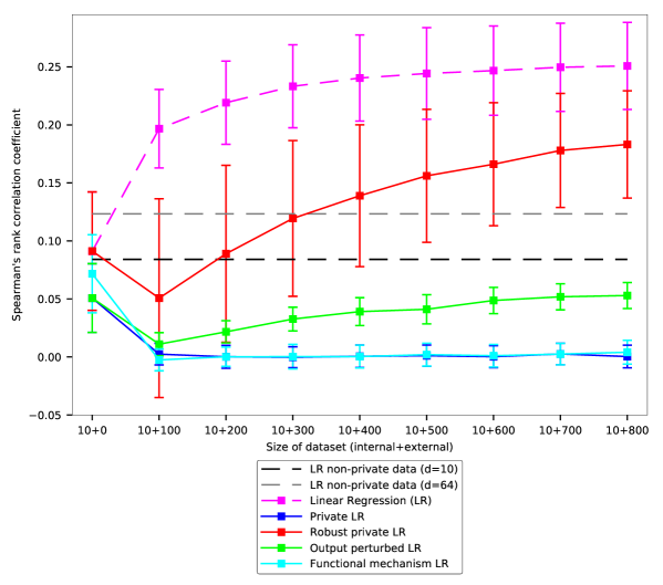
Figure 6: This is a complement to Figure 2 with more stringent privacy. Here we show Spearman’s rank correlation coefficients ($\rho$) between the measured ranking of the cell lines and the ranking predicted by the models using $\epsilon=1$. The baselines (horizontal dashed lines) are learned on 10 non-private data points; the private algorithms additionally have privacy-protected data (x-axis). The non-private algorithm (LR) has the same amount of additional non-privacy-protected data. All methods use 10-dimensional data except purple baseline showing the best performance with 10 non-private data points. The results are averaged over all drugs and 50-fold Monte Carlo cross-validation; error bars denote standard deviation over 50 Monte Carlo repeats. The result shows that more data are needed for good prediction performance under more stringent privacy.

References

- [1] R. Bayardo and R. Agrawal. Data privacy through optimal k-anonymization. In Proc. 21st Int. Conf. Data Eng. (ICDE 2005), 2005.
- [2] A. Blum, C. Dwork, F. McSherry, and K. Nissim. Practical privacy: the SuLQ framework. In Proc. PODS 2005, 2005.
- [3] K. Chaudhuri and C. Monteleoni. Privacy-preserving logistic regression. In Adv. Neural Inf. Process. Syst. 21, 2008.
- [4] J. C. Costello, L. M. Heiser, E. Georgii, M. Gönen, M. P. Menden, N. J. Wang, M. Bansal, M. Ammad-ud din, P. Hintsanen, S. A. Khan, J.-P. Mpindi, O. Kallioniemi, A. Honkela, T. Aittokallio, K. Wennerberg, NCI DREAM Community, J. J. Collins, D. Gallahan, D. Singer, J. Saez-Rodriguez, S. Kaski, J. W. Gray, and G. Stolovitzky. A community effort to assess and improve drug sensitivity prediction algorithms. Nat. Biotechnol., 32(12):1202–1212, Dec 2014.
- [5] P. Diaconis and D. Ylvisaker. Conjugate priors for exponential families. Ann. Stat., 7(2):269–281, Mar 1979.
- [6] J. C. Duchi, M. I. Jordan, and M. J. Wainwright. Privacy aware learning. J. ACM, 61(6):1–57, Dec 2014.
- [7] C. Dwork, F. McSherry, K. Nissim, and A. Smith. Calibrating noise to sensitivity in private data analysis. In Proc. TCC 2006. 2006.
- [8] C. Dwork and A. Roth. The algorithmic foundations of differential privacy. Found. Trends Theor. Comput. Sci., 9(3-4):211–407, Aug. 2014.
- [9] J. Foulds, J. Geumlek, M. Welling, and K. Chaudhuri. On the theory and practice of privacy-preserving Bayesian data analysis. In Proc. UAI 2016, Mar. 2016. arXiv:1603.07294.
- [10] M. Fredrikson, E. Lantz, S. Jha, S. Lin, D. Page, and T. Ristenpart. Privacy in pharmacogenetics: An end-to-end case study of personalized warfarin dosing. In Proc. 23rd USENIX Security Symp. (USENIX Security 2014), pages 17–32, 2014.
- [11] M. J. Garnett et al. Systematic identification of genomic markers of drug sensitivity in cancer cells. Nature, 483(7391):570–575, Mar 2012.
- [12] C. Gentry. A fully homomorphic encryption scheme. PhD thesis, Stanford University, 2009.
- [13] M. Gymrek, A. L. McGuire, D. Golan, E. Halperin, and Y. Erlich. Identifying personal genomes by surname inference. Science, 339(6117):321–324, Jan 2013.
- [14] A. Harmanci and M. Gerstein. Quantification of private information leakage from phenotype-genotype data: linking attacks. Nat. Methods, 13(3):251–256, Mar 2016.
- [15] N. Homer et al. Resolving individuals contributing trace amounts of DNA to highly complex mixtures using high-density SNP genotyping microarrays. PLoS Genet., 4(8):e1000167, Aug 2008.
- [16] A. Kucukelbir, D. Tran, R. Ranganath, A. Gelman, and D. M. Blei. Automatic differentiation variational inference. J Mach Learn Res, 18(14):1–45, 2017.
- [17] N. Li, T. Li, and S. Venkatasubramanian. t-closeness: Privacy beyond k-anonymity and l-diversity. In Proc. ICDE 2007, 2007.
- [18] A. Machanavajjhala, D. Kifer, J. Gehrke, and M. Venkitasubramaniam. L-diversity: Privacy beyond k-anonymity. TKDD, 1(1):3, Mar 2007.
- [19] M. Naveed et al. Privacy in the genomic era. ACM Comput. Surv., 48(1):1–44, Aug 2015.
- [20] J. Salvatier, T. V. Wiecki, and C. Fonnesbeck. Probabilistic programming in Python using PyMC3. PeerJ Computer Science, 2:e55, apr 2016.
- [21] M. Schmidt, E. van den Berg, M. Friedlander, and K. Murphy. Optimizing costly functions with simple constraints: A limited-memory projected quasi-newton algorithm. In Proc. AISTATS 2009, 2009.
- [22] A. Smith. Efficient, differentially private point estimators. Sept. 2008. arXiv:0809.4794 [cs.CR].
- [23] Y.-X. Wang, J. Lei, and S. E. Fienberg. Learning with differential privacy: Stability, learnability and the sufficiency and necessity of ERM principle. Feb. 2015. arXiv: 1502.06309 [stat.ML].
- [24] L. Wasserman and S. Zhou. A statistical framework for differential privacy. J. Am. Stat. Assoc., 105(489):375–389, Mar 2010.
- [25] O. Williams and F. McSherry. Probabilistic inference and differential privacy. In Adv. Neural Inf. Process. Syst. 23, 2010.
- [26] X. Wu, M. Fredrikson, W. Wu, S. Jha, and J. F. Naughton. Revisiting differentially private regression: Lessons from learning theory and their consequences. Dec. 2015. arXiv:1512.06388 [cs.CR].
- [27] W. Yang et al. Genomics of drug sensitivity in cancer (GDSC): a resource for therapeutic biomarker discovery in cancer cells. Nucleic Acids Res., 41(Database issue):D955–D961, Jan 2013.
- [28] J. Zhang, Z. Zhang, X. Xiao, Y. Yang, and M. Winslett. Functional mechanism: Regression analysis under differential privacy. PVLDB, 5(11):1364–1375, 2012.
- [29] Z. Zhang, B. Rubinstein, and C. Dimitrakakis. On the differential privacy of Bayesian inference. In Proc. AAAI 2016, 2016.