Comparative study of Weyl semimetal, topological and Chern insulators: thin-film point of view

Abstract

Regarding three-dimensional (3D) topological insulators and semimetals as a stack of constituent 2D topological (or sometimes non-topological) systems is a useful viewpoint. Here, we perform a comparative study of the paradigmatic 3D topological phases: Weyl semimetal (WSM), strong vs. weak topological insulators (STI/WTI), and Chern insulator (CI). By calculating the $\mathbb{Z}$- and $\mathbb{Z}_{2}$-indices for the thin films of such 3D topological phases, we follow dimensional evolution of topological properties from 2D to 3D. It is shown that the counterpart of STI and WTI in the time-reversal symmetry broken CI system are, respectively, WSM and CI phases. The number ${\cal N}_{D}$ of helical Dirac cones emergent on the surface of a topological insulator is shown to be identical to the number ${\cal N}_{W}$ of the pairs of Weyl cones in the corresponding WSM phase: ${\cal N}_{D}={\cal N}_{W}$. To test the robustness of this scenario against disorder, we have studied the transport property of disordered WSM thin films, taking into account both the bulk and surface contributions.

I Introduction

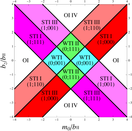
(a) (b)

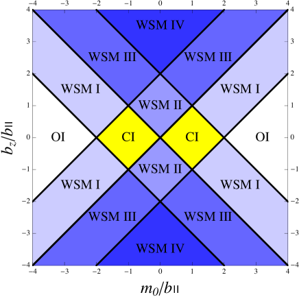
Figure 1: Phase diagram of (a) WTI/STI type model (class AII) and (b) CI/WSM type model (class A). The two panels are based on a specific model defined, respectively, in Eqs. (1) and (15). The Roman numbers: I, II, III, IV, indicated in each region represent, in panel (a) the number ${\cal N}_{D}$ of helical Dirac cones emergent on the $[001]$ surface, while in panel (b) the number ${\cal N}_{W}$ of the pairs of Weyl nodes. They are identical in WTI/STI phase and in the corresponding CI/WSM phase.

Weyl semimetal is a topologically nontrivial gapless phase. Hosur and Qi (2013) For theorists it is almost trivially an interesting topic to study since it is exotic; it has been repeatedly shown that the existence of Weyl and Dirac cones in the band structure results in anomalous spectral and transport properties. Geim and Novoselov (2007); Qi and Zhang (2011); Hosur and Qi (2013) Recently, it is becoming also a target of active experimental study; cf., its experimental discovery in the system of TaAs Lv et al. (2015); Xu et al. (2016a, b) and NbAs.Xu et al. (2015) In this paper, we highlight the physics of Weyl semimetal (WSM) in its relation to its prototypical gapped analogue, the topological insulator from the viewpoint of thin-film construction.

The appearance of Weyl points in the band structure has been already mentioned in Ref. Murakami, 2007. A few years later, the existence of WSM phase has been pointed out in a pyrochlore iridate. Wan et al. (2011) Recently, WSM has been predicted numerically in Ta-, Nb-, and Mo-based compounds. Weng et al. (2015); Sun et al. (2015); Huang et al. (2015) WSM is also shown to be robust against disorder. Kobayashi et al. (2014); Ominato and Koshino (2014); Nandkishore et al. (2014); Syzranov et al. (2015); Roy and Das Sarma (2014); Sbierski et al. (2014)

The 3D topological insulator is realized in a time-reversal symmetric system. It is also under the influence of spin-orbit coupling, and belongs to symmetry class AII. The time-reversal operator $\Theta$ of the system satisfies $\Theta^{2}=-1$, and the topological number used for distinguishing the two types of insulating phases; one with the surface state, the other without, is of the $\mathbb{Z}_{2}$-type. Such $\mathbb{Z}_{2}$-type topological insulator has also subclasses: strong and weak topological insulators (STI and WTI). From a theoretical point of view it is natural to construct such STI and WTI phases by stacking 2D quantum spin Hall (QSH) layers. The QSH phase can be regarded as a 2D version of the $\mathbb{Z}_{2}$ topological insulator. Such TI thin films, or stacked QSH layers has been much studied theoretically, Lu et al. (2010); Linder et al. (2009); Liu et al. (2010a); Shan et al. (2010); Ebihara et al. (2012); Okamoto et al. (2014); Sacksteder et al. (2015) and experimentally as well. Zhang et al. (2010); Hirahara et al. (2010); Taskin et al. (2012); Nguyen et al. (2016)

What happens if we stack quantum anomalous Hall (QAH) layers instead of the QSH layers? The resulting 3D system is typically a Chern insulator (CI), characterized by a $\mathbb{Z}$-type topological index, but it can be also a WSM; the coupling between the layers may turn the system to be a semimetal [cf., typical phase diagram shown in Fig. 1(b)]. By its construction the entire class of models breaks time-reversal symmetry and belongs to the symmetry class A. Here, we attempt to make a close analogy between the two types of constructions: i.e., for (a) WTI/STI vs. (b) CI/WSM type models.

In the two panels of Fig. 1, a typical phase diagram of the above two types of models is shown. In panel (a) WTI phases are located at the central area of topologically nontrivial region. Topologically more robust STI phases appear at the periphery of such WTI phases. Such an arrangement of the phases may seem to be natural, if one considers that as varying the model parameters through WTI$\rightarrow$STI$\rightarrow$OI regions, the number of Dirac cones emergent on the surface decreases monotonically as 2$\rightarrow$1$\rightarrow$0. In this sense STI may be regarded as partially broken WTI. In a similar, but more definite sense specified below, WSM can be regarded as partially broken CI.

Panel (b) of Fig. 1 shows a typical phase diagram of the CI/WSM type model. Here, we have adjusted the model parameters so that it looks almost identical to panel (a), the phase diagram for the WTI/STI type model. Indeed, they are identical except that in panel (b) WTI and STI are replaced, respectively, with CI and WSM phases. In CI, stacked chiral edge modes are all intact, while in WSM, they survive only in a part of the 2D surface Brillouin zone (BZ); in a finite range of $k_{z}$ between the two Weyl points, they form Fermi arc surface states. Indeed in the process of stacking chiral edge modes some of them become gapped in WSM. Here, in this work we clarify how this precisely happens by closely examining the dimensional crossover of topological signatures (see Fig. 3).

Finally, to test the robustness of our scenario, we have also performed a numerical study on the transport property of disordered WSM thin films. Here, we have considered the conductance of the system in the presence of both the bulk and surface contributions. The (two-terminal) conductance of the system has been calculated using the transfer matrix method, and compared with topological index maps (Sec. IV).

II Model Hamiltonian and phase diagram

II.1 WTI and STI as stacked QSH layers

The standard recipe for constructing a $\mathbb{Z}_{2}$-type topological insulator is to employ a Wilson-Dirac type effective Hamiltonian, Zhang et al. (2009); Liu et al. (2010b)

$$H^{\rm TI}_{\rm bulk}(\bm{k})=m_{\rm 3D}(\bm{k})\beta+\!\!\!\sum_{\mu=x,y,z}\!t_{\mu}\sin k_{\mu}\alpha_{\mu},$$ (1)

where

$$m_{\rm 3D}(\bm{k})=m_{0}-\sum_{\mu=x,y,z}b_{\mu}\cos k_{\mu},$$ (2)

is the Wilson-Dirac mass. The anti-commuting $4\times 4$ matrices $\alpha_{\mu}$ and $\beta$ can be written as a product of two Pauli matrices, $\sigma_{\mu}$ and $\tau_{\mu}$, each representing spin and orbital, as

$$\alpha_{\mu}=\tau_{x}\otimes\sigma_{\mu},\>\ \beta=\tau_{z}\otimes 1_{2}.$$ (3)

By changing the ratio of $m_{0}$ and $b_{\mu}$ in Eq. (2) one can realize various different STI and WTI phases [see phase diagram shown in Fig. 1(a)]. Imura et al. (2012) In Fig. 1(a) only the effects of uni-axial anisotropy $b_{z}/b_{\parallel}$ is taken into account, setting

$$b_{x}=b_{y}=b_{\parallel}.$$ (4)

Together with strong and weak indices: $\nu_{0}$ and $(\nu_{1},\nu_{2},\nu_{3})$, the number ${\cal N}_{D}$ of helical Dirac cones emergent on either the top or bottom surface is shown by the Roman numbers in each of STI and WTI phases.

The tight-binding form of the bulk effective Hamiltonian Eq. (1) can be used for implementing a thin-film geometry:

$$H^{\rm TI}_{\rm film}(\bm{k}_{\rm 2D})=1_{N_{z}}\!\otimes\!\left(m_{\rm 2D}(\bm{k}_{\rm 2D})\beta+\sum_{\mu=x,y}t_{\mu}\sin k_{\mu}\alpha_{\mu}\right)$$

$$-{b_{z}\over 2}\!\left(\begin{array}[]{c@{\ }c@{\ }c@{\ }c@{\,}}0&1&&\\[-5.69054pt] 1&\ddots&\ddots&\\[-5.69054pt] &\ddots&\ddots&1\\ &&1&0\end{array}\right)\!\!\otimes\!\beta+{t_{z}\over 2}\!\left(\begin{array}[]{c@{\ }c@{\ }c@{\ }c@{\,}}0&-i&&\\[-5.69054pt] i&\ddots&\ddots&\\[-5.69054pt] &\ddots&\ddots&-i\\[0.0pt] &&i&0\end{array}\right)\!\!\otimes\!\alpha_{z},$$ (13)

where

$$m_{\rm 2D}(\bm{k}_{\rm 2D})=m_{0}-\sum_{\mu=x,y}b_{\mu}\cos k_{\mu}$$ (14)

represents a 2D version of the Wilson-Dirac mass, Eq. (2) for each of the constituent layers, while the first part of the direct products represent the layer degrees of freedom. In Eq. (13) we have truncated the system in the number of stacking layers $N_{z}$.

Note that in Fig. 1(a) the $b_{z}/b_{\parallel}=1$ line corresponds to the isotropic case, representing the 3D limit, while the $b_{z}/b_{\parallel}=0$ line represents a strong anisotropy limit, where the phase diagram becomes identical to that of the 2D limit. Since $m_{\rm 2D}(\bm{k}_{\rm 2D})$ encodes topological nature of each constituent layer, the phase boundaries in the 2D limit are determined by the zeros of $m_{\rm 2D}(\bm{k}_{\rm 2D})$ at the four TRIM in 2D. They are indeed at $m_{0}/b_{\parallel}=-2,0,2$.

II.2 CI and WSM as stacked QAH layers

As one of the simplest realization of WSM with broken time reversal symmetry (class A), we consider the two-band Hamiltonian of the multi-layer CI model: Yang et al. (2011); Imura and Takane (2011); Shapourian and Hughes (2016); Chen et al. (2015); Liu et al. (2016)

$$H^{\rm CI}_{\rm bulk}({\bm{k}})=m_{\rm 3D}(\bm{k})\sigma_{z}+\sum_{\mu=x,y}t_{\mu}\sin{k_{\mu}}\sigma_{\mu},$$ (15)

where $m_{\rm 3D}(\bm{k})$ is the one given in Eq. (2) and $\sigma_{\mu}$ are Pauli matrices.

In parallel with the conversion from Eq. (1) to Eq. (13), the thin-film version of Eq. (15) reads,

$$H^{\rm CI}_{\rm film}(\bm{k}_{\rm 2D})= \ 1_{N_{z}}\otimes\left(m_{\rm 2D}(\bm{k}_{\rm 2D})\sigma_{z}+\sum_{\mu=x,y}t_{\mu}\sin{k_{\mu}}\sigma_{\mu}\right)$$

$$-\frac{b_{z}}{2}\begin{pmatrix}0&1&&\\[-2.84526pt] 1&\ddots&\ddots&\\[-2.84526pt] &\ddots&\ddots&1\\ &&1&0\end{pmatrix}\otimes\sigma_{z}.$$ (16)

Here, the first line of the right-hand side of the equation represents a contribution from each QAH layer.Qi et al. (2006) QAH is a 2D version of $\mathbb{Z}$ type topological insulator characterized by $\mathbb{Z}$ type topological index. The Hamiltonian Eq. (16) represents stacked QAH layers.

In the limit of $b_{z}\rightarrow 0$, each of such QAH layers decouples, representing the 2D limit of the model. The abscissa of the phase diagram (the $b_{z}/b_{\parallel}=0$ line) shown in Fig. 1(b) falls on this case, exhibiting two different QAH regions: one with $\sigma_{xy}=+e^{2}/h$ ($m_{0}/b_{\parallel}\in[0,2]$), the other with $\sigma_{xy}=-e^{2}/h$ ($m_{0}/b_{\parallel}\in[-2,0]$). As a finite layer coupling $b_{z}$ is introduced, these two QAH phases evolve into CI phases. These are 3D topological phases that have fully inherited the 2D-type topological character of the constituent QAH phase; for each $k_{z}$ in the BZ, the system shows a QAH effect, exhibiting a gapless chiral edge mode.

Yet, as $b_{z}$ is increased, (i) a pair of Weyl points [or (ii) two pairs of Weyl points] appear, depending on the value of $m_{0}/b_{\parallel}$: e.g., for $b_{z}/b_{\parallel}=1$, case (i) $m_{0}/b_{\parallel}\in[1,3]$ or $[-3,-1]$, while case (ii) $m_{0}/b_{\parallel}\in[-1,1]$ in the bulk 3D BZ, driving the system into a semi-metallic (gapless) phase. The Weyl points appear at $k_{z}=\pm k_{0}$, with (i) $\bar{\Gamma}$ or $\bar{M}$: $(k_{x},k_{y})=(0,0)$ or $(\pi,\pi)$, (ii) $\bar{X}$ and $\bar{Y}$: $(k_{x},k_{y})=(\pi,0)$ and $(0,\pi)$. These WSM phases can be regarded as partially broken CI in the sense that in these phases the 2D topological character of the constituent QAH layers is only partially maintained. In CI phases any slice of the system at a given $k_{z}$ in the BZ, say, the entire BZ is topologically nontrivial, while in the WSM phase only a part of the BZ, $k_{z}\in[-k_{0},k_{0}]$, is topologically nontrivial; a gapless surface, connecting the Weyl cones to form the so-called Fermi arc, appears.

(a)

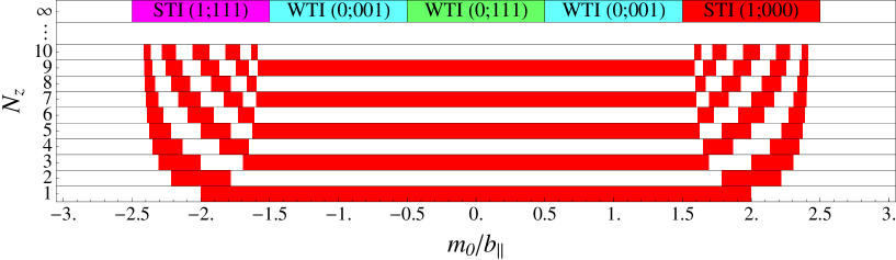
(b)

Figure 2: $\mathbb{Z}_{2}$-index map in case of (a) an anisotropic: $b_{z}/b_{\parallel}=0.5$ vs. (b) the isotropic: $b_{z}/b_{\parallel}=1$ choice of parameters. The red [white] region corresponds to the range of QSH ($\nu=1$) [OI ($\nu=0$)]. The stripe pattern in the central region represents an even-odd feature of the 2D $\mathbb{Z}_{2}$ character QSH/OI, while a mosaic-like feature is also characteristic at both ends of the stripe. The mosaic pattern corresponds to the the STI phase in the 3D limit. The precise nature of the mosaic pattern depends on the SOC hopping parameter $t_{z}$, here set to be $t_{z}/b_{\parallel}=0.5$.

(a)

(b)

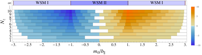
(c)

Figure 3: $\mathbb{Z}$-index map, representing the dimensional crossover of topological signatures in the CI/WSM class of models (symmetry class A). The three panels correspond to the cases of (a) $b_{z}/b_{\parallel}=0.5$, (b) $b_{z}/b_{\parallel}=1$, (c) $b_{z}/b_{\parallel}=1.5$.

As in the case of Fig. 1(a), in Fig. 1(b), the fully anisotropic line ($b_{z}/b_{\parallel}=0$) corresponds to the 2D limit of the phase diagram, while the isotropic line ($b_{z}/b_{\parallel}=1$) corresponds to the purely 3D limit. A thin-film situation may fall on halfway between these two limits. Indeed, evolution of the phases in Figs. 1(a) and 1(b) from $b_{z}/b_{\parallel}=0$ to $b_{z}/b_{\parallel}=1$ can be interpreted as representing a dimensional crossover of the system from 2D to 3D. Scheurer et al. (2015); Kobayashi et al. (2015) In the following section we examine this point more closely by explicitly studying the evolution of 2D topological signatures in a concrete thin-film situation at a varying number of stacking layers.

III Mapping the topological index: $\mathbb{Z}_{2}$- and $\mathbb{Z}$-index maps

Thin films of WTI/STI and CI/WSM can be regarded as 2D $\mathbb{Z}_{2}$- and $\mathbb{Z}$- type topological insulators, or an effective 2D QSH or QAH system. To characterize them we introduce and calculate $\mathbb{Z}_{2}$- and $\mathbb{Z}$- topological indices Bernevig et al. (2006); Qi et al. (2006); Thouless et al. (1982) adapted to such thin-film systems.

III.1 $\mathbb{Z}_{2}$-index map for the WTI/STI class

In case of the WTI/STI type models as defined in Eq. (13), we can define and calculate a 2D $\mathbb{Z}_{2}$-type topological index $\nu$ as given in Ref. Kobayashi et al., 2015. Here, we recalculate the same index using the convention of Eq. (13) at different mass parameters and at different numbers of stacked layers. Also, following the same reference, we plot the data in the form of “$\mathbb{Z}_{2}$-index map”, in the space of $m_{0}/b_{\parallel}$ vs. $N_{z}$: the number of stacked layers. Examples of such $\mathbb{Z}_{2}$-index maps are shown in Fig. 2.

The last row ($N_{z}=1$) of the index map represents the appearance of QSH vs. OI phases in the 2D limit, while the remaining part of the map shows how this distribution evolves as a function of $N_{z}$. Globally, one can recognize two types of patterns in this map: stripe vs. mosaic-like irregular patterns. The locations of the two patterns on the map indicate roughly the positions of WTI and STI phases in the 3D limit; the appearance of a mosaic pattern is a precursor of STI phase in the 3D limit, while a stripe pattern implies the existence of WTI phase in the same limit (see Fig. 2). While these two patterns reflect the topological features in the 3D limit, they have a slight difference in their physical origins.

The mosaic pattern in the $\mathbb{Z}_{2}$-index map is due to hybridization of the top and bottom surface wave functions in the thin film geometry; it represents how the surface state wave functions penetrate into the bulk. Though surface states of an STI and of a WTI are localized in the vicinity of the surface, they do have a finite penetration length. The penetration of the surface state wave function is not necessary a simple exponential decay, but it can show a damped oscillation. The appearance of a mosaic pattern in the $\mathbb{Z}_{2}$-index map happens precisely in the latter case. Naturally, the depth of penetration and the oscillation pattern depends on the choice of parameters, so does the resulting mosaic pattern. In the present model whether the surface state wave function show damped oscillation or overdamping depends on the ratio $t_{z}/b_{z}$ (see Appendix A for details). This surface/bulk mechanism for the mosaic pattern stands, naturally, when the given set of parameters corresponds to a situation in which a surface state appears on the $[001]$ surface in the 3D limit.

The physical origin of the stripe pattern is, on the contrary, much related to the edge modes in the thin-film construction. As far as the low-energy transport properties are concerned, stacked QSH layers can be regarded as coupled 1D helical modes. On one hand, such coupled 1D modes hybridize and become gapped when $N_{z}$ is even, while a single gapless mode remains when $N_{z}$ is odd. Ringel et al. (2012); Matsumoto et al. (2015); Takane (2016) This is typically the situation that underlies a stripe pattern in the $\mathbb{Z}_{2}$-index map. On the other hand, stacked QSH layers lead to a WTI in the 3D limit, in which coupled 1D helical modes evolve into two helical Dirac cones that appear on side surfaces of a WTI. Therefore, a stripe pattern in the $\mathbb{Z}_{2}$-index map implies the existence of a WTI phase in the 3D limit.

However, precisely speaking, this edge picture for the stripe pattern is justified only when $[001]$ surface is gapped [this is indeed the case in the WTI $(0;001)$ phase] in our construction. Note that in Fig. 2 the stripe pattern in panel (a) corresponds to the WTI $(0;001)$ phase in the range of parameters $-1.5<m_{0}/b_{\parallel}<-0.5$ and $0.5<m_{0}/b_{\parallel}<1.5$, while in panel (b) the same pattern corresponds to the WTI $(0;111)$ phase in the 3D limit. In the second regime the above criterion is no longer legitimate, but it still shows a stripe pattern. In the Appendix we show that the stripe pattern in this case can be understood in the surface/bulk picture. Indeed, a complete interpretation of the two patterns in the $\mathbb{Z}_{2}$-index map involves a more thorough examination of the two scenarios: bulk/surface vs. edge points of view as described in Appendix A. It is shown that the two pictures are complementary in the formation of the two patterns. Also, this complementarity can be regarded as a manifestation of the guiding principle, the bulk-boundary correspondence, Hatsugai (1993) which is generic to all types of topological quantum phenomena, here in the formation of mosaic vs. stripe patterns.

III.2 $\mathbb{Z}$-index map for the CI/WSM class

In case of the CI/WSM type model of thin-film as defined in Eq. (16), we can define and characterize its thin-film by a 2D $\mathbb{Z}$-index,Thouless et al. (1982) again at different mass parameters and at different numbers of stacked layers. We then plot the index in the same way as we did for the $\mathbb{Z}_{2}$-type models to form of a $\mathbb{Z}$-index map. Some examples of the $\mathbb{Z}$-index map are shown in Fig. 3. Thanks to the notation used in Eqs. (15) and (1), the similarity of the two models is explicit. Recall also the similarity and correspondence at the level of the phase diagram (see Fig. 1).

The $\mathbb{Z}$-index, or the Chern number is defined in terms of Berry curvature integrated over the entire BZ. Thouless et al. (1982) Yet, a non-vanishing contribution arises only from singularities of the band structure, i.e., from Dirac cones. The so-called “Dirac cone argument” allows for expressing the Chern number as a sum of contributions from such Dirac cones. Oshikawa (1994); Hatsugai et al. (1996) In the case of Wilson-Dirac type models on a cubic/square lattice the Dirac cones appear only on the four inversion symmetric points in the BZ, and correspondingly, the expression for the related $\mathbb{Z}$- and $\mathbb{Z}_{2}$-indices simplifies significantly. Imura et al. (2010)

III.2.1 $\mathbb{Z}$-index map, the edge point of view, comparison of the two maps

A single layer of the CI/WSM film prescribed by Eq. (16) is nothing but the QAH insulator studied in Ref. Yoshimura et al., 2014. Here, following Ref. Yoshimura et al., 2014 we express the Chern number ${\cal N}$ in terms of the band index $\delta_{\bm{k}}=\pm 1$ at the inversion symmetric points: $\Gamma(0,0)$, X$(\pi,0)$, Y$(0,\pi)$ and M$(\pi,\pi)$ in the following way:

$${\cal N}={1\over 2}\delta_{\Gamma}+{1\over 2}\delta_{\rm X}+{1\over 2}\delta_{\rm Y}+{1\over 2}\delta_{\rm M}.$$ (17)

At the neighborhood of the four Dirac points ${\bm{k}}_{D}$ ($D=\Gamma$, X, Y, M), ${\bm{k}}={\bm{k}}_{D}+{\bm{p}}$, Eq. (16) can be expressed as follows,

$$H({\bm{k}}_{D}\!+\!{\bm{p}})=\tilde{t}_{x}p_{x}\sigma_{x}+\tilde{t}_{y}p_{y}\sigma_{y}+\left(\tilde{m}+O(|\bm{p}|^{2})\right)\sigma_{z},$$ (18)

by using ${\bm{k}}\cdot{\bm{p}}$-approximation. The specific values of $\tilde{t}_{x}$, $\tilde{t}_{y}$ and $\tilde{m}$ for each symmetric points ${\bm{k}}_{D}$ are shown in TABLE 1. Then one can define $\delta_{\bm{k}}$ such that

$$\delta_{\bm{k}}=-{\rm sgn}[\tilde{t}_{x}]{\rm sgn}[\tilde{t}_{y}]{\rm sgn}[\tilde{m}].$$ (19)

Table 1: List of $\tilde{t}_{x}$, $\tilde{t}_{y}$ and $\tilde{m}$ at four Dirac points ${\bm{k}}_{D}$

${\bm{k}}_{D}$		$\tilde{t}_{x}$		$\tilde{t}_{y}$		$\tilde{m}$
$(0,0)$		$t_{x}$		$t_{y}$		$m_{0}-b_{x}-b_{y}$
$(\pi,0)$		$-t_{x}$		$t_{y}$		$m_{0}+b_{x}-b_{y}$
$(0,\pi)$		$t_{x}$		$-t_{y}$		$m_{0}-b_{x}+b_{y}$
$(\pi,\pi)$		$-t_{x}$		$-t_{y}$		$m_{0}+b_{x}+b_{y}$

The single-layer QAH model is also a specific spin sector of the BHZ model. Naturally, the phase diagrams of the two models resemble each other. In the QAH model, simply the two QSH phases of the BHZ are replaced with two different QAH phases with $\sigma_{xy}=\pm e^{2}/h$. In the $\mathbb{Z}$-index map shown in Fig. 3 the bottom line represents the single-layer case, exhibiting two types of QAH phases with

$$\sigma_{xy}={\cal N}{e^{2}\over h}=\pm{e^{2}\over h}$$ (20)

in the range of parameters, respectively, $m_{0}/b_{\parallel}\in[0,2]$ and $m_{0}/b_{\parallel}\in[-2,0]$.

As more layers are stacked, contributions of different layers accumulate, but they also sometime interfere, resulting in a partial or full cancellation of a non-trivial contribution. In the presence of such interference, the Chern number ${\cal N}$ is at most equal to $N_{z}$ (in magnitude). In the $\mathbb{Z}$-index map shown in Fig. 3, regions of larger Chern number ${\cal N}$ are indicated by a thicker color. In the case of $\mathbb{Z}_{2}$-type models, the interference of contributions of the neighboring layers is determined by the competition of two types of hopping terms: $t_{z}$ and $b_{z}$ in the stacking direction.Kobayashi et al. (2015) Here, in the $\mathbb{Z}$-type case the $t_{z}$-type hopping is absent by construction, so that formulations developed in the Appendix of Ref. Kobayashi et al., 2015 become simpler. The thin-film Hamiltonian $H_{\rm film}$ for the CI/WSM case can be made block diagonal by a simpler procedure, i.e.,

$$\left(P\otimes 1_{2}\right)^{\dagger}H_{\rm film}(\bm{k}_{\rm 2D})\left(P\otimes 1_{2}\right)=$$

$$\begin{pmatrix}H_{q_{1}}(\bm{k}_{\rm 2D})&&&\\ &\!H_{q_{2}}(\bm{k}_{\rm 2D})&&\\ &&\!\ddots&\\ &&&\!H_{q_{N_{z}}}(\bm{k}_{\rm 2D})\end{pmatrix},$$ (21)

where the orthogonal matrix $P$ takes the following form; its $(n,l)$-element is given by

$$P_{nl}=\sqrt{\frac{2}{N_{z}+1}}\sin{\left(\frac{nl}{N_{z}+1}\pi\right).}$$ (22)

Thus, contributions from different layers $l=1,2,\cdots,N_{z}$, are rearranged into those from different sectors $q_{j}=-(N_{z}+1)/2+j$ $(j=1,2,\cdots,N_{z})$, and in this $q_{j}$-representation they decouple:

$${\cal N}=\sum_{l=1}^{N_{z}}{\cal N}_{q_{j}},$$ (23)

where ${\cal N}_{q_{j}}$ is a contribution from the ${q_{j}}$-th sector, determined by the ${q_{j}}$-th diagonal block of the diagonalized Hamiltonian, Eq. (21), which takes the following $2\times 2$ matrix form:

$$H_{q_{j}}(\bm{k}_{\rm 2D})=m_{q_{j}}(\bm{k}_{\rm 2D})\sigma_{z}+\sum_{\mu=x,y}t_{\mu}\sin{k_{\mu}}\sigma_{\mu},$$ (24)

where

$$m_{q_{j}}(\bm{k}_{\rm 2D})=m_{0}-b_{\parallel}\sum_{\mu=x,y}\cos{k_{\mu}}-b_{z}\cos{\frac{j\pi}{N_{z}+1}}.$$ (25)

Due to the last term of Eq. (25), which we will call

$$\Delta m_{q_{j}}=b_{z}\cos\frac{j\pi}{N_{z}+1},$$ (26)

the location of two QAH regions are shifted by the amount ${\Delta m_{q_{j}}\over b_{\parallel}}$; i.e.,

$${\cal N}_{q_{j}}=+1\quad{\rm if}\quad{m_{0}\over b_{\parallel}}\in\left[{\Delta m_{q_{j}}\over b_{\parallel}},2+{\Delta m_{q_{j}}\over b_{\parallel}}\right],$$ (27)

while

$${\cal N}_{q_{j}}=-1\quad{\rm if}\quad{m_{0}\over b_{\parallel}}\in\left[-2+{\Delta m_{q_{j}}\over b_{\parallel}},{\Delta m_{q_{j}}\over b_{\parallel}}\right].$$ (28)

Note that $\Delta m_{q_{j}}$ is the counterpart of $\lambda_{q_{j}}$ for the $\mathbb{Z}_{2}$-type model given in Eq. (31) of Ref. Kobayashi et al., 2015. Thus, contributions from different sectors $q_{j}=-(N_{z}-1)/2,-(N_{z}-1)/2+1,\cdots,(N_{z}-1)/2$, are superposed and interfere, resulting in a pattern of the $\mathbb{Z}$-index map as shown in Fig. 3. The overall structure of the $\mathbb{Z}$-index map is much similar to that of the $\mathbb{Z}_{2}$-index map, except that the latter is in bicolor while the former is in multicolor. Yet, apart from that distribution pattern of different topological numbers is much alike. One can recognize the same two characteristic patterns: stripe vs. mosaic, which was important in the interpretation of the $\mathbb{Z}_{2}$-index map, here also in the $\mathbb{Z}$-index map.

In the three panels of Fig. 3, an even/odd feature, or a stripe pattern appears in the central region; here, we are referring to an even/odd feature embedded in the (globally) mosaic pattern, somewhat analogous to the one seen in the WTI $(0;111)$ phase in Fig. 5. This even/odd feature is a result of the cancellation between ${\cal N}_{q_{j}}$ and ${\cal N}_{-q_{j}}$ ($=-{\cal N}_{q_{j}}$), i.e., cancellation between the edge modes of opposite chiralities in this range of parameters. If $N_{z}$ is even, this cancellation is complete, while if $N_{z}$ is odd, the central term ${\cal N}_{0}$ remains. The width of the ${\cal N}=0$ region becomes narrower as $N_{z}$ is increased even if $N_{z}$ is even. The width is determined by the last cancelling pairs, ${\cal N}_{1/2}$ and ${\cal N}_{-1/2}$, and therefore given as

$$\frac{\Delta m_{-1/2}}{b_{\parallel}}-\frac{\Delta m_{1/2}}{b_{\parallel}}={b_{z}\over b_{\parallel}}\sin{\pi\over 2(N_{z}+1)}.$$ (29)

Comparing $\Delta m_{q_{j}}$ given in Eq. (26) with Eqs. (31) and (32) of Ref. Kobayashi et al., 2015, one can verify that all the phase boundaries of the $\mathbb{Z}_{2}$-index map as shown in Fig. 2 reduce to those of the corresponding $\mathbb{Z}$-index map in the limit of $t_{z}\rightarrow 0$. To make this analogy more explicit we have added weak-like indices Yoshimura et al. (2014) on the $\mathbb{Z}_{2}$-index map [see Figs. 5(a) and 5(b) in Appendix].

III.2.2 Back to the bulk-boundary relations, complementarity of the two pictures

We have so far made a close comparison of $\mathbb{Z}$- and $\mathbb{Z}_{2}$-index maps mainly from the viewpoint of edge mechanism (at least from the $\mathbb{Z}$-side). The edge picture we have been based on in the description of the $\mathbb{Z}$-index map is an approach starting from the 2D limit, i.e., an approach following the evolution of edge properties in the process of stacking more and more layers. The conspicuous even-odd feature emergent in the middle of the mosaic-like pattern formed at the merger of the ${\cal N}>0$ and ${\cal N}<0$ sides was understood from this point of view. While, in the previous subsection the mosaic pattern on the $\mathbb{Z}_{2}$-side has been discussed from the viewpoint of surface/bulk picture, i.e., in terms of the damped-oscillatory pattern of the top-bottoms surface wave function, penetrating through the bulk of the film to attain the opposite surface, leading to peculiar oscillatory (mosaic) pattern of the hybridization gap. Since the mosaic pattern on the $\mathbb{Z}_{2}$-side reduces to that of the $\mathbb{Z}$-side in the limit of $t_{z}\rightarrow 0$, it is natural to assume that the mosaic pattern on the $\mathbb{Z}$-side can also be understood from such a surface/bulk point of view. However, one may realize in a moment that this might not be the case, since on the $\mathbb{Z}$-side, i.e., in the CI/WSM film the top-bottoms surfaces are always gapped, so that a priori there is not even a starting point for developing a similar surface/bulk picture.

This apparent contradiction can be resolved as follows. The penetration of the top-bottom surface wave function in the WTI/STI model becomes deeper as the magnitude of SOC hopping $t_{z}$ is diminished. In the limit of $t_{z}\rightarrow 0$, the surface wave function evolves continuously into a bulk wave function associated with a pair of new bulk Dirac points.

Let us start with the STI $(1;000)$ phase represented by the point: $(m_{0}/b_{\parallel},b_{z}/b_{\parallel})=(2,1)$ in Fig. 1(a). On top and bottom surfaces of the relatively thick film (or slab) placed normal to the $z$-axis, the surface Dirac cone appears at the $\bar{\Gamma}$-point: $(k_{x},k_{y})=(0,0)$. The phase boundaries of Fig. 1(a) correspond to either of the gap closing points of Eq. (1) at one of the eight time reversal invariant momenta (TRIM) in the 3D BZ: $k_{\mu}=0,\pi$. Conversely, as far as $t_{\mu}$ is finite, gap closing of Eq. (1) occurs only at such 8 TRIM. However, in the limit of $t_{z}\rightarrow 0$, chance for a new type of gap closing arises, i.e., at $k_{z}\neq 0,\pi$; indeed, at

$$k_{z}=\pm\arccos\left({m_{0}\over b_{z}}-2{b_{\parallel}\over b_{z}}\right)\equiv\pm k_{0},$$ (30)

or at the value of $k_{z}$ satisfying

$${m_{0}\over b_{\parallel}}-2={b_{z}\over b_{\parallel}}\cos k_{z}.$$ (31)

In the isotropic case: $b_{z}/b_{\parallel}=1$ the STI $(1;000)$ phase corresponds to the range: $1<m_{0}/b_{\parallel}<3$; therefore, the left-hand side of the equation is between 1 and $-1$. Thus, $k_{0}$ satisfying the condition (31) always exists in the interval: $[-\pi,\pi]$. In the limit of $t_{z}\rightarrow 0$, the top and bottom surface wave functions reduce to the following bulk wave functions associated with these new Weyl points that appear at $k_{z}=\pm k_{0}$, i.e.,

$$\psi(z)=A\sin(k_{0}\pm q)z,$$ (32)

where $q$ is a dips from the Weyl point determined by the boundary condition: $\psi(N_{z}+1)=0$. Imura et al. (2012)

The number ${\cal N}_{D}$ of surface Dirac cones that appear on top and bottom surfaces of the slab differ in different phases of Fig. 1(a). The above argument shows that the number ${\cal N}_{W}$ of Weyl pairs that appear in each of the WSM phase in Fig. 1(b) coincide with the number ${\cal N}_{D}$ of the corresponding WTI/STI phase:

$${\cal N}_{D}={\cal N}_{W}.$$ (33)

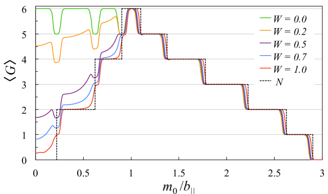
Figure 4: Conductance for CI/WSM thin-films. The two-terminal conductance $G$ for a system of $N_{x}=200$, $N_{y}=50$, $N_{z}=6$ is plotted in units of $e^{2}/h$ at different values of disorder strength $W$. The dotted line represents the change of bulk topological $\mathbb{Z}$-index, extracted from Fig. 3(b).

IV Effects of disorder and relation to experiments

The above $\mathbb{Z}$- and $\mathbb{Z}_{2}$-index maps are closely related to conductance of the system. Kobayashi et al. (2015) By calculating the conductance, we can also discuss how robust the characteristic features such as the stripe vs. mosaic patterns emergent in the $\mathbb{Z}$- and $\mathbb{Z}_{2}$-index maps are in the presence of disorder. Here we compare closely the topological (i.e., $\mathbb{Z}$- or $\mathbb{Z}_{2}$-) index vs. conductance in the CI/WSM case. A similar study of conductance maps has been done in Ref. Kobayashi et al., 2015 in the case of WTI/STI thin-films. The advantage of the conductance map is that one can equally consider the case of zero and finite disorder on the same footing.

Here, we focus on the behavior of the two-terminal conductance $G$ calculated in the transfer matrix approach employed in Ref. Kobayashi et al., 2015. $G$ has been calculated for a rectangular: $N_{x}\times N_{y}\times N_{z}$ with the three axes $x$, $y$, $z$, placed respectively in the direction of $x$: conduction, $y$: width and $z$: stacking. Here, we set $b_{z}/b_{\parallel}=1$. The conductance has been studied in detail for a system of $N_{x}=200$, $N_{y}=50$ and several different $N_{z}$. In Fig. 4 the calculated conductance $G$ at $N_{z}=6$ at the varying ratio of mass and Wilson parameters ($m_{0}/b_{\parallel}$) is shown. Different curves correspond to different strength of disorder $W$; here we consider site disorder, i.e., random potential on each site, obeying the uniform distribution $[-W/2,W/2]$. For curves with $W\neq 0$ an average over independent configurations of disorder is taken for 10 samples. In Fig. 4 the calculated conductance curves are plotted against a dotted line; the latter represents the change of the bulk topological $\mathbb{Z}$-index, extracted from Fig. 3(b).

For sufficiently large $N_{x}$ and $N_{y}$, the $\mathbb{Z}$-index map coincides identically with the Hall conductance ($G_{H}$) map. On the other hand, here we consider the two-terminal conductance $G$. In Fig. 4 let us first note that the step structure on the outer side of the $\mathbb{Z}$-index map starting at $m_{0}/b_{\parallel}=3.0$ is well reproduced in the conductance calculation. This is so, since in the regime of $m_{0}/b_{\parallel}\gtrsim 1$, only edge modes of the same chirality are responsible for conduction. We then note that in the central mosaic region ($m_{0}/b_{\parallel}\lesssim 1$), the discrepancy of the two maps arises. In this region the Chern number $\cal N$ (or equivalently $G_{H}$) decreases as $m_{0}/b_{\parallel}$ decreases, forming the inner staircase of the map, while in conductance map, $G$ is kept at the maximal saturated value in the clean limit $W=0$. This is because $G$ measures only the number of transmitting channels; here they are edge modes circulating around the periphery of the film-bar shaped sample. By its nature, $G$ is insensitive to the chirality of edge modes.Kane and Mele (2005) If ${\cal N}_{+}$ (${\cal N}_{-}$) edge modes of the $+$ ($-$) chirality are available for conduction, the Hall conductance is given as

$$G_{H}=({\cal N}_{+}-{\cal N}_{-}){e^{2}\over h}={\cal N}{e^{2}\over h},$$ (34)

while the two-terminal conductance becomes

$$G=({\cal N}_{+}+{\cal N}_{-}){e^{2}\over h}.$$ (35)

In the clean limit $W=0$, a few (here, in the case of $N_{z}=6$, three) pairs of counter-propagating modes are circulating, practically without backscattering (since the bulk is gapped). Only at the value of $m_{0}/b_{\parallel}$ corresponding to the steps, the bulk becomes gapless, allowing for weak backscattering through the bulk, which explains small deviation of $G$ at $W=0$ from the maximal value $G=6$ in the vicinity of these values of $m_{0}/b_{\parallel}$.

As disorder is increased, the value of $G$ decrease to the value predicted by the $\mathbb{Z}$-index map in the central mosaic area, corresponding to the WSM phase. This is because of the backscattering between the counter propagating chiral states due to disorder, resulting in $G=|{\cal N}_{+}-{\cal N}_{-}|{e^{2}\over h}$. The typical mosaic-stripe pattern characteristic to WSM thin-films is a feature, albeit predicted by the $\mathbb{Z}$-index map, manifesting only on addition of finite disorder, and in this sense, may be called an emergent property induced by the interplay of nontrivial topological nature of WSM and disorder.

Let us note here that a step-like change of the conductance somewhat reminiscent of the ones shown in Fig. 4 has been reported in a slightly different context.Burkov and Balents (2011); Xu et al. (2011) However, the step structure reported in these references appears as varying the thickness of the film, and is associated with quantization of $k_{z}$ due to the finite thickness. On the other hand, the step structure shown in Fig. 4 is due to gradual destruction of the CI phase in the process of becoming a WSM, and occurs at a fixed $N_{z}$. In this sense the nature of the step structure shown in Fig. 4 is qualitatively different from the ones reported in Refs. Burkov and Balents, 2011 and Xu et al., 2011.

V Concluding remarks

In this paper, a comparative study of the CI/WSM and WTI/STI type topological insulators and semimetals has been done from the viewpoint of thin-film construction. We introduced a correspondence relation between the two classes of models, based on a specific model defined in Sec. II and the corresponding phase diagram shown in Fig. 1. In particular, we have argued that the counter part of STI and WTI in the time-reversal symmetry (TRS) broken class is, respectively, WSM and CI phase. We have also demonstrated that STI can be regarded as partially broken WTI, and in the same way WSM can be regarded as partially broken CI. Much of the subsequent analysis was developed, based on this parallelism.

Here, let us comment on how generic this correspondence relation could be. Naturally, the exact correspondence of the two phase diagrams shown in Fig. 1 is due to a specific choice of our model. Yet, the comparison and the analogy developed in this analysis could be more generic and valid for a broad class of TRS broken WSM phases. Starting with the time-reversal symmetric limit, let us imagine adding a perturbation that breaks TRS. Then, the concept of STI and WTI is invalidated since TRS is no longer existent. Still, in some cases a specific type of WTI phase is not much affected by such a perturbation, but simply replaced with a CI phase. On the other hand, surrounding STI phases disappear immediately as the TRS breaking perturbation turned on. Burkov and Balents (2011) They are considered to be generically transformed to a WSM phase. Then, it is likely that one ends up, at least, qualitatively, with the same situation as described by the model employed here. The situation would be much different if one considers WSM of the inversion symmetry (IS) breaking type. Herring (1937) In the limit of both TRS and IS preserved, STI and WTI phases are separated by a Dirac semimetal (DSM) line. Adding IS breaking perturbation does not generically destroy STI and WTI phases, while a finite WSM phase replacing the DSM line appears in between. Such a finite WSM region appears also between STI and OI phases.

To reveal the dimensional crossover of topological signatures in the two class of models, we have focused on the thin-film construction of the two types of models. To quantify the crossover, we have focused on the dimensional crossover of topological signatures in the two class of models. To quantify this, we have introduced, and then evaluated the 2D topological indices of $\mathbb{Z}$- and $\mathbb{Z}_{2}$ types, characterizing the system. We mapped such topological indices ($\mathbb{Z}$- and $\mathbb{Z}_{2}$-index maps) as a function of the gap parameter and film thickness, to reveal characteristic global patterns, such as stripe or mosaic patterns, encoding the topological properties of the system in the 3D limit. The nature of the two characteristic patterns are discussed and understood from two complementary points of view: surface/bulk vs. edge pictures. The similarity and relation of the $\mathbb{Z}$- and $\mathbb{Z}_{2}$-type index maps are discussed and clarified.

It was shown that in the limit of $t_{z}\rightarrow 0$ essentially all the phase boundaries of the $\mathbb{Z}_{2}$-index map coincide with those of the $\mathbb{Z}$-index map. We have demonstrated how surface helical Dirac cones emergent and protected on the surface of an STI evolve and eventually transform into a pair of Weyl cones in the bulk of the WSM. The number of surface Dirac cones ${\cal N}_{D}$ on the surface of an STI, or of WTI in some cases, is identical to the number of Weyl cone pairs ${\cal N}_{W}$ lurking in the bulk of the corresponding WSM.

Finally, to check the robustness of our findings against disorder and their relevance to experiments we have also made a close comparison of the topological $\mathbb{Z}$-index map (in the clean limit) with the corresponding conductance map at varying strength of disorder. Compared with the previously studied case of WTI/STI thin-films, Kobayashi et al. (2015) in which the correspondence between the two-terminal conductance map at finite disorder with the topological $\mathbb{Z}_{2}$-index map was apparent, here in the present CI/WSM case studied in detail in the previous section the correspondence between the conductance and $\mathbb{Z}$-index maps is only partial in the clean limit, since as discussed in the previous section, the $\mathbb{Z}$-index map should show a perfect correspondence with the Hall conductance map. Yet, we have argued that the two-terminal conductance at varying strength of disorder those features that we have revealed in the study of $\mathbb{Z}$-index map appears as an emergent property, which manifests only at some finite strength of disorder.

(a)

(b)

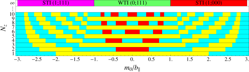
Figure 5: $\mathbb{Z}_{2}$-index map with 2D weak-like indices Kobayashi et al. (2015). The yellow (cyan/red) region corresponds to the range of $\nu=1$ ($\nu=0$), corresponding to red (white) regions in Fig. 2. The red region represents the 2D weak phase.

Appendix A Surface/bulk vs. edge picture for the $\mathbb{Z}_{2}$-index map

A.1 Nature of the mosaic pattern: the surface/bulk mechanism

On the isotropic line: $b_{z}=b_{\parallel}$, the range of parameter: $1<m_{0}/b_{\parallel}<3$ corresponds to an STI phase with a surface Dirac cone at the $\bar{\Gamma}$-point. Imura et al. (2012) Let us examine in this case whether hybridization of the top and bottom surface wave functions in the thin-film geometry leads to inversion of the valence and conduction bands, characteristic to an effective QSH state.

The surface wave function in the semi-infinite geometry takes the following form:

$$\psi(z)\propto\rho_{1}^{z}-\rho_{2}^{z},$$ (36)

where $\rho_{1,2}$ are two solutions to a characteristic equation associated with the surface wave function at $E=0$, i.e.,

$$\rho_{1,2}={\pm\sqrt{D}-(m_{0}-2b_{\parallel})\over b_{z}-t_{z}},$$ (37)

with the discriminant $D$ given as

$$D=(m_{0}-2b_{\parallel})^{2}+t_{z}^{2}-b_{z}^{2}.$$ (38)

The double sign in the numerator defines, respectively, $\rho_{1}$ and $\rho_{2}$. Here, the system is assumed to be extended, e.g., on the $z>0$ side with a surface at $z=0$. To be consistent with this boundary condition the surface wave function (36) is constructed in such a way that it vanishes at $z=0$: $\psi(0)=0$, but decays exponentially as $z\rightarrow\infty$. Such a surface solution is possible, when the magnitude of two solutions $\rho_{1,2}$ in Eq. (37) are both smaller than unity: $|\rho_{1,2}|<1$, which is indeed possible in the present case: $1<m_{0}/b_{\parallel}<3$.

It can be shown that the sign and magnitude of the energy gap $\Delta E$ of a TI thin-film of a thickness $N_{z}$ is related to those of the surface wave function $\psi(z)$ of an auxiliary semi-infinite system at the depth of the film thickness $N_{z}$, or more directly to $\rho_{1,2}$ as Okamoto et al. (2014)

$$\Delta E(N_{z}) = E_{c}-E_{v}$$ (39)

$$= A\left(\rho_{1}^{N_{z}+1}-\rho_{2}^{N_{z}+1}\right)$$

$$\propto \psi(N_{z}+1),$$

where $A$ is a positive constant. When $\Delta E<0$ ($\Delta E>0$) the TI thin-film realizes an effective 2D QSH (ordinary) insulator. Shan et al. (2010)

It will be convenient to consider the cases of (i) $t_{z}<b_{z}$ and (ii) $t_{z}>b_{z}$ separately, since the profile of the $\mathbb{Z}_{2}$-index map changes qualitatively, depending on the sign of $t_{z}-b_{z}$. If (i) $t_{z}<b_{z}$, the two solutions $\rho_{1,2}$ may have an imaginary part since $D$ can be negative; in this case $\rho_{1,2}$ becomes a pair of conjugate complex numbers [see Eq. (37)]. Then, the corresponding surface wave function $\psi(z)$ becomes oscillatory, showing a damped oscillation, i.e., the wave function changes its sign in a somewhat irregular way as it penetrates into the bulk. When the thickness $N_{z}$ of the film is chosen such that $\psi(N_{z}+1)<0$, the hybridization gap $\Delta E$ becomes negative [see Eq. (39)], implying that the film is in the QSH phase. The corresponding $\mathbb{Z}_{2}$-index map shows a mosaic pattern.

If (ii) $t_{z}>b_{z}$, on the other hand, the two solutions $\rho_{1,2}$ are always real since $D$ is always positive. They are also positive and negative value solutions: $\rho_{1}=\rho_{+}>0$ and $\rho_{2}=-\rho_{-}<0$. In this case the corresponding surface wave function is overdamped. Yet, the wave function can still be oscillatory in some cases. Let us recall that if (a) $m_{0}-2b_{\parallel}>0$, the system is on the OI side in the 2D limit. Eq. (37) implies that $\rho_{+}>\rho_{-}$ in this case, therefore, the corresponding surface wave function in the form of Eq. (36) is always positive. The resulting $\mathbb{Z}_{2}$-index map shows a trivial pattern.

If (b) $m_{0}-2b_{\parallel}<0$, on the other hand, the system is on the QSH side in the 2D limit. In this case the weight of the two solutions are inverted, i.e., the opposite inequality, $\rho_{+}<\rho_{-}$ stands. Then, the corresponding surface wave function

$$\psi(z)=\rho_{+}^{z}-(-\rho_{-})^{z}$$ (40)

shows an alternating sign. In the $\mathbb{Z}_{2}$-index map, an alternating series of QSH and OI layers appear, forming a peculiar stripe pattern.

A.2 Crossover from mosaic to stripe pattern: complementarity of the two pictures

When $t_{z}<b_{z}$, there exists an interval:

$$\!2-\sqrt{\left({b_{z}\over b_{\parallel}}\right)^{\!\!2}\!-\!\left({t_{z}\over b_{\parallel}}\right)^{\!\!2}}<{m_{0}\over b_{\parallel}}<2+\sqrt{\left({b_{z}\over b_{\parallel}}\right)^{\!\!2}\!-\!\left({t_{z}\over b_{\parallel}}\right)^{\!\!2}},$$ (41)

in which damped oscillation of the surface wave function leads to a mosaic pattern of the $\mathbb{Z}_{2}$-index map. Note that the interval Eq. (41) fits inside the window of the STI phase: $1<m_{0}/b_{\parallel}<3$. The interval Eq. (41) corresponds to the range of parameters in which $D<0$, so that $\rho_{1,2}$ become a pair of conjugate complex numbers, resulting in a damped oscillation of the surface wave function. The corresponding $\mathbb{Z}_{2}$-index map shows a mosaic pattern. Beyond the interval Eq. (41) and inside the STI window the surface wave function shows a feature analogous to the case of $t_{z}>b_{z}$, which means that a stripe pattern appears on the side of $m_{0}-2b_{\parallel}<0$. To be precise, a mosaic pattern appears only when $N_{z}$ is sufficiently large even in the interval (41). Recall that the film thickness $N_{z}$ is discretized to be an integer multiple of the layer separation $a$, which is here chosen to be unity. Due to this discreteness of $N_{z}$, evolution of the $\mathbb{Z}_{2}$-index at small $N_{z}$ is superficially periodic in spite of the damping. The resulting pattern is also practically indistinguishable from a perfect stripe pattern. Aperiodicity becomes manifest, however, at finite $N_{z}$ and a crossover from a mosaic to a stripe pattern occurs. The boundary between the mosaic and stripe pattern approaches an asymptotic line in the limit of large $N_{z}$, corresponding to either of the extremities of the interval (41).

The interval (41) appears as a finite range of $m_{0}/b_{\parallel}$ in the STI window: $1<m_{0}/b_{\parallel}<3$ in the range: $0<t_{z}<b_{z}$. In the limit of $t_{z}\rightarrow 0$ the interval dominates the entire STI window; a mosaic pattern becomes predominant in the STI region. The interval (41) vanishes, on the other hand, as $t_{z}$ approaches $b_{z}$; i.e., the mosaic pattern disappears at $t_{z}=b_{z}$. The situation is unchanged even when $t_{z}$ is further increased.

Such an observation shows that the extremity of the STI window toward the boundary to the neighboring WTI phase: $-1<m_{0}/b_{\parallel}<1$, is necessarily be ended by a stripe pattern. The origin of this stripe pattern is a particular oscillation pattern of the surface wave function in the form of Eq. (40). Last but not least, this stripe pattern continues on the WTI side beyond the boundary at $m_{0}/b_{\parallel}=1$. This is because the surface states at $\bar{\Gamma}$ on two surfaces of the film is no longer existent; there are still two Dirac cones on the WTI side but they appear at $\bar{X}=(\pi,0)$ and $\bar{Y}=(0,\pi)$, and no more at $\bar{\Gamma}$. Since there is no more surface state at $\bar{\Gamma}$, no more gap inversion occurs at $\bar{\Gamma}$. There still can occur band inversions at $\bar{X}$ and $\bar{Y}$, but at least on the isotropic line they occur simultaneously at the two points; therefore, irrelevant to the $\mathbb{Z}_{2}$-index map shown in Fig. 2. In Fig. 5 2D weak-like indices Yoshimura et al. (2014) are added to the the $\mathbb{Z}_{2}$-index map shown in Fig. 2. This introduces an additional mosaic-like structure in the WTI $(0;111)$ region stemming from the band inversion at $\bar{X}$ and $\bar{Y}$ points.

We have so far seen that the stripe pattern in the WTI $(0;111)$ region as shown in Fig. 2 can be regarded as a heritage of the same pattern at an extremity of the neighboring STI phase. The stripe pattern in the WTI phase is also sometimes understood from the viewpoint of edge wave functions emergent on narrow side surfaces of the film. Imura et al. (2012) In this second point of view only edge/side-surface properties are involved, while the present scenario involves only the penetration of the top-bottom-surface wave function into the bulk. This complementarity of the two pictures is the hallmark of all topological quantum phenomena, often referred to as the bulk-boundary correspondence. Hatsugai (1993)

In the above surface/bulk point of view, the stripe pattern in the WTI $(0;111)$ region as shown in Fig. 2 can be regarded as a heritage of the same pattern at an extremity of the neighboring STI phase. In Sec. III A we have seen that the stripe pattern in the WTI phase can be also sometimes understood from the viewpoint of edge wave functions emergent on narrow side surfaces of the film. This complementarity of the edge vs. surface/bulk pictures can be regarded as a manifestation of the bulk-boundary correspondence, Hatsugai (1993); Wen (2007) which is believed to be the hallmark of all topological properties.

References

- Hosur and Qi (2013) P. Hosur and X. Qi, Comptes Rendus Physique 14, 857 (2013), ISSN 1631-0705, topological insulators / Isolants topologiquesTopological insulators / Isolants topologiques, URL http://www.sciencedirect.com/science/article/pii/S1631070513001710.
- Geim and Novoselov (2007) A. K. Geim and K. S. Novoselov, Nat Mater 6, 183 (2007), URL http://dx.doi.org/10.1038/nmat1849.
- Qi and Zhang (2011) X.-L. Qi and S.-C. Zhang, Rev. Mod. Phys. 83, 1057 (2011), URL http://link.aps.org/doi/10.1103/RevModPhys.83.1057.
- Lv et al. (2015) B. Q. Lv, N. Xu, H. M. Weng, J. Z. Ma, P. Richard, X. C. Huang, L. X. Zhao, G. F. Chen, C. E. Matt, F. Bisti, et al., Nat Phys 11, 724 (2015).
- Xu et al. (2016a) S.-Y. Xu, I. Belopolski, D. S. Sanchez, M. Neupane, G. Chang, K. Yaji, Z. Yuan, C. Zhang, K. Kuroda, G. Bian, et al., Phys. Rev. Lett. 116, 096801 (2016a), URL http://link.aps.org/doi/10.1103/PhysRevLett.116.096801.
- Xu et al. (2016b) N. Xu, H. M. Weng, B. Q. Lv, C. E. Matt, J. Park, F. Bisti, V. N. Strocov, D. Gawryluk, E. Pomjakushina, K. Conder, et al., Nat Commun 7 (2016b).
- Xu et al. (2015) S.-Y. Xu, N. Alidoust, I. Belopolski, Z. Yuan, G. Bian, T.-R. Chang, H. Zheng, V. N. Strocov, D. S. Sanchez, G. Chang, et al., Nat Phys 11, 748 (2015).
- Murakami (2007) S. Murakami, New Journal of Physics 9, 356 (2007), URL http://stacks.iop.org/1367-2630/9/i=9/a=356.
- Wan et al. (2011) X. Wan, A. M. Turner, A. Vishwanath, and S. Y. Savrasov, Phys. Rev. B 83, 205101 (2011), URL http://link.aps.org/doi/10.1103/PhysRevB.83.205101.
- Weng et al. (2015) H. Weng, C. Fang, Z. Fang, B. A. Bernevig, and X. Dai, Phys. Rev. X 5, 011029 (2015), URL http://link.aps.org/doi/10.1103/PhysRevX.5.011029.
- Sun et al. (2015) Y. Sun, S.-C. Wu, M. N. Ali, C. Felser, and B. Yan, Phys. Rev. B 92, 161107 (2015), URL http://link.aps.org/doi/10.1103/PhysRevB.92.161107.
- Huang et al. (2015) S.-M. Huang, S.-Y. Xu, I. Belopolski, C.-C. Lee, G. Chang, B. Wang, N. Alidoust, G. Bian, M. Neupane, C. Zhang, et al., Nat Commun 6 (2015).
- Kobayashi et al. (2014) K. Kobayashi, T. Ohtsuki, K.-I. Imura, and I. F. Herbut, Phys. Rev. Lett. 112, 016402 (2014), URL http://link.aps.org/doi/10.1103/PhysRevLett.112.016402.
- Ominato and Koshino (2014) Y. Ominato and M. Koshino, Phys. Rev. B 89, 054202 (2014), URL http://link.aps.org/doi/10.1103/PhysRevB.89.054202.
- Nandkishore et al. (2014) R. Nandkishore, D. A. Huse, and S. L. Sondhi, Phys. Rev. B 89, 245110 (2014), URL http://link.aps.org/doi/10.1103/PhysRevB.89.245110.
- Syzranov et al. (2015) S. V. Syzranov, V. Gurarie, and L. Radzihovsky, Phys. Rev. B 91, 035133 (2015), URL http://link.aps.org/doi/10.1103/PhysRevB.91.035133.
- Roy and Das Sarma (2014) B. Roy and S. Das Sarma, Phys. Rev. B 90, 241112 (2014), URL http://link.aps.org/doi/10.1103/PhysRevB.90.241112.
- Sbierski et al. (2014) B. Sbierski, G. Pohl, E. J. Bergholtz, and P. W. Brouwer, Phys. Rev. Lett. 113, 026602 (2014), URL http://link.aps.org/doi/10.1103/PhysRevLett.113.026602.
- Lu et al. (2010) H.-Z. Lu, W.-Y. Shan, W. Yao, Q. Niu, and S.-Q. Shen, Phys. Rev. B 81, 115407 (2010).
- Linder et al. (2009) J. Linder, T. Yokoyama, and A. Sudbø, Phys. Rev. B 80, 205401 (2009).
- Liu et al. (2010a) C.-X. Liu, H. Zhang, B. Yan, X.-L. Qi, T. Frauenheim, X. Dai, Z. Fang, and S.-C. Zhang, Phys. Rev. B 81, 041307 (2010a), URL http://link.aps.org/doi/10.1103/PhysRevB.81.041307.
- Shan et al. (2010) W.-Y. Shan, H.-Z. Lu, and S.-Q. Shen, New Journal of Physics 12, 043048 (2010).
- Ebihara et al. (2012) K. Ebihara, K. Yada, A. Yamakage, and Y. Tanaka, Physica E: Low-dimensional Systems and Nanostructures 44, 885 (2012).
- Okamoto et al. (2014) M. Okamoto, Y. Takane, and K.-I. Imura, Phys. Rev. B 89, 125425 (2014).
- Sacksteder et al. (2015) V. Sacksteder, T. Ohtsuki, and K. Kobayashi, Phys. Rev. Applied 3, 064006 (2015), URL http://link.aps.org/doi/10.1103/PhysRevApplied.3.064006.
- Zhang et al. (2010) Y. Zhang, K. He, C.-Z. Chang, C.-L. Song, L.-L. Wang, X. Chen, J.-F. Jia, Z. Fang, X. Dai, W.-Y. Shan, et al., Nature Physics 6, 584 (2010).
- Hirahara et al. (2010) T. Hirahara, Y. Sakamoto, Y. Takeichi, H. Miyazaki, S.-i. Kimura, I. Matsuda, A. Kakizaki, and S. Hasegawa, Phys. Rev. B 82, 155309 (2010), URL http://link.aps.org/doi/10.1103/PhysRevB.82.155309.
- Taskin et al. (2012) A. A. Taskin, S. Sasaki, K. Segawa, and Y. Ando, Phys. Rev. Lett. 109, 066803 (2012).
- Nguyen et al. (2016) T.-A. Nguyen, D. Backes, A. Singh, R. Mansell, C. Barnes, D. A. Ritchie, G. Mussler, M. Lanius, D. Grützmacher, and V. Narayan, Scientific Reports 6, 27716 EP (2016).
- Zhang et al. (2009) H. Zhang, C.-X. Liu, X.-L. Qi, X. Dai, Z. Fang, and S.-C. Zhang, Nature physics 5, 438 (2009).
- Liu et al. (2010b) C.-X. Liu, X.-L. Qi, H. Zhang, X. Dai, Z. Fang, and S.-C. Zhang, Phys. Rev. B 82, 045122 (2010b), URL http://link.aps.org/doi/10.1103/PhysRevB.82.045122.
- Imura et al. (2012) K.-I. Imura, M. Okamoto, Y. Yoshimura, Y. Takane, and T. Ohtsuki, Phys. Rev. B 86, 245436 (2012), URL http://link.aps.org/doi/10.1103/PhysRevB.86.245436.
- Yang et al. (2011) K.-Y. Yang, Y.-M. Lu, and Y. Ran, Phys. Rev. B 84, 075129 (2011), URL http://link.aps.org/doi/10.1103/PhysRevB.84.075129.
- Imura and Takane (2011) K.-I. Imura and Y. Takane, Phys. Rev. B 84, 245415 (2011), URL http://link.aps.org/doi/10.1103/PhysRevB.84.245415.
- Shapourian and Hughes (2016) H. Shapourian and T. L. Hughes, Phys. Rev. B 93, 075108 (2016), URL http://link.aps.org/doi/10.1103/PhysRevB.93.075108.
- Chen et al. (2015) C.-Z. Chen, J. Song, H. Jiang, Q.-f. Sun, Z. Wang, and X. C. Xie, Phys. Rev. Lett. 115, 246603 (2015), URL http://link.aps.org/doi/10.1103/PhysRevLett.115.246603.
- Liu et al. (2016) S. Liu, T. Ohtsuki, and R. Shindou, Phys. Rev. Lett. 116, 066401 (2016), URL http://link.aps.org/doi/10.1103/PhysRevLett.116.066401.
- Qi et al. (2006) X.-L. Qi, Y.-S. Wu, and S.-C. Zhang, Phys. Rev. B 74, 085308 (2006), URL http://link.aps.org/doi/10.1103/PhysRevB.74.085308.
- Scheurer et al. (2015) M. S. Scheurer, S. Rachel, and P. P. Orth, Sci. Rep. 5, 8386 (2015).
- Kobayashi et al. (2015) K. Kobayashi, Y. Yoshimura, K.-I. Imura, and T. Ohtsuki, Phys. Rev. B 92, 235407 (2015), URL http://link.aps.org/doi/10.1103/PhysRevB.92.235407.
- Bernevig et al. (2006) B. A. Bernevig, T. L. Hughes, and S.-C. Zhang, Science 314, 1757 (2006), ISSN 0036-8075, eprint http://science.sciencemag.org/content/314/5806/1757.full.pdf, URL http://science.sciencemag.org/content/314/5806/1757.
- Thouless et al. (1982) D. J. Thouless, M. Kohmoto, M. P. Nightingale, and M. den Nijs, Phys. Rev. Lett. 49, 405 (1982), URL http://link.aps.org/doi/10.1103/PhysRevLett.49.405.
- Ringel et al. (2012) Z. Ringel, Y. E. Kraus, and A. Stern, Phys. Rev. B 86, 045102 (2012), URL http://link.aps.org/doi/10.1103/PhysRevB.86.045102.
- Matsumoto et al. (2015) A. Matsumoto, T. Arita, Y. Takane, Y. Yoshimura, and K.-I. Imura, Phys. Rev. B 92, 195424 (2015), URL http://link.aps.org/doi/10.1103/PhysRevB.92.195424.
- Takane (2016) Y. Takane, Journal of the Physical Society of Japan 85, 013706 (2016), eprint http://dx.doi.org/10.7566/JPSJ.85.013706, URL http://dx.doi.org/10.7566/JPSJ.85.013706.
- Hatsugai (1993) Y. Hatsugai, Phys. Rev. Lett. 71, 3697 (1993), URL http://link.aps.org/doi/10.1103/PhysRevLett.71.3697.
- Oshikawa (1994) M. Oshikawa, Phys. Rev. B 50, 17357 (1994), URL http://link.aps.org/doi/10.1103/PhysRevB.50.17357.
- Hatsugai et al. (1996) Y. Hatsugai, M. Kohmoto, and Y.-S. Wu, Phys. Rev. B 54, 4898 (1996), URL http://link.aps.org/doi/10.1103/PhysRevB.54.4898.
- Imura et al. (2010) K.-I. Imura, A. Yamakage, S. Mao, A. Hotta, and Y. Kuramoto, Phys. Rev. B 82, 085118 (2010), URL http://link.aps.org/doi/10.1103/PhysRevB.82.085118.
- Yoshimura et al. (2014) Y. Yoshimura, K.-I. Imura, T. Fukui, and Y. Hatsugai, Phys. Rev. B 90, 155443 (2014), URL http://link.aps.org/doi/10.1103/PhysRevB.90.155443.
- Kane and Mele (2005) C. L. Kane and E. J. Mele, Phys. Rev. Lett. 95, 226801 (2005), URL http://link.aps.org/doi/10.1103/PhysRevLett.95.226801.
- Burkov and Balents (2011) A. A. Burkov and L. Balents, Phys. Rev. Lett. 107, 127205 (2011), URL http://link.aps.org/doi/10.1103/PhysRevLett.107.127205.
- Xu et al. (2011) G. Xu, H. Weng, Z. Wang, X. Dai, and Z. Fang, Phys. Rev. Lett. 107, 186806 (2011), URL http://link.aps.org/doi/10.1103/PhysRevLett.107.186806.
- Herring (1937) C. Herring, Phys. Rev. 52, 365 (1937), URL http://link.aps.org/doi/10.1103/PhysRev.52.365.
- Wen (2007) X.-G. Wen, Quantum Field Theory of Many-Body Systems (OXFORD UNIVERSITY PRESS, http://www.oupcanada.com/catalog/9780199227259.html, 2007), 1st ed., ISBN 9780199227259.