Parallax and orbital effects in astrometric microlensing with binary sources

Abstract

In gravitational microlensing, binary systems may act as lenses or sources. Identifying lens binarity is generally easy especially in events characterized by caustic crossing since the resulting light curve exhibits strong deviations from smooth single-lensing light curve. On the contrary, light curves with minor deviations from a Paczyński behaviour do not allow one to identify the source binarity. A consequence of the gravitational microlensing is the shift of the position of the multiple image centroid with respect to the source star location - the so called astrometric microlensing signal. When the astrometric signal is considered, the presence of a binary source manifests with a path that largely differs from that expected for single-source events. Here, we investigate the astrometric signatures of binary sources taking into account their orbital motion and the parallax effect due to the Earth motion, which turn out not to be negligible in most cases. We also show that considering the above-mentioned effects is important in the analysis of astrometric data in order to correctly estimate the lens-event parameters.

1 Introduction

Gravitational microlensing is a mature technique for detecting compact objects in the disk and in the halo of our Galaxy via the observation of the light magnification of source stars due to the intervening lenses. Indeed, the technological instrument advances allowed gravitational microlensing to detect and characterized low-mass objects (see e.g. Park et al. 2015) as well as binary lens systems (see e.g. Udalski et al. 2015) including planetary systems with planets masses down to Earth mass with host-planet separations of about a few AU.

In addition to the magnification of the source brightness, another phenomenon related to microlensing is the shift of the light centroid of the source images. This subject was studied by many authors (see e.g. Walker 1995, Miyamoto & Yoshii 1995, Høg et al. 1995, Jeong et al. 1995, Paczyński 1996, Paczyński 1998, Dominik & Sahu 2000, Takahashi 2003, Lee et al. 2010). In the simplest case of a point lens, lensing causes the source image to split into two and the position of the light centroid with respect to the unlensed source star position traces out an ellipse with semi-axes depending, in general, on the lens impact parameter $u_{0}$ (the minimum projected distance of the lens to the source star) and the shape of the astrometric trajectory does not depend on the Einstein time $t_{E}$.

When the lens is a binary system (see e.g. Han et al. 1999, Safizadeh et al. 1999, Han et al. 2001, Bozza 2001, Hideki 2002, Sajadian & Rahvar 2015), the number and the position of the images differ from those of the single lens case and the astrometric signal trajectory and the deviation varies depending on on the binary system parameters (i.e., the mass ratio and the component separation).

It is evident that in both cases astrometry gives more information than that derived from the analysis of light curves (photometry), allowing one to better constrain the lens system.

A further advantage of the astrometric microlensing is that an event is potentially observable for a much longer time with respect to the typical photometric event because astrometric signals persit to much longer lens-source separations than photometric signals (see next sections). In addition, interesting events can be predicted in advance (Paczyński 1995) and, indeed, by studying in detail the characteristics of stars with large proper motions, Proft et al. (2011) identified dozens of candidates for astrometric microlensing observations using the Gaia satellite, an European Space Agency (ESA) mission, that is performing photometry, spectroscopy and high precision astrometry (Eyer et al. 2013).

Binary star systems can act as sources of microlensing events. In this regard, each component of the binary system acts as an independent source (with given impact parameter) for the intervening lens and the resultinng light curve corresponds to a a superposition of the single-lensing light curves associated with the individual source stars. However, although Griest & Hu (1992) predicted that about $10\%$ of the observable events should involve features of a binary source, few clear detection of such systems was claimed up today. As argued by Dominik (1998 b), the lack of binary source events may be explained by the fact that most of the light curves for events involving a binary source can be explained by single lens model with a blended source. So, binary sources are hidden in photometric observations. This is certainly not the case for astrometric microlensing observations, for which, as first pointed out by Han & Kim (1999) and Dalal & Griest (2001), the binarity of the source strongly modifies astrometric signals. However, these authors accounted for the binary source effect by considering the centroid shift as due mainly to the primary object while treating its companion as a simple blending source. This simplifying assumption is overcome in the present paper where both components of the binary source and their relative motion are considered in calculating the resulting astrometric path.

Several theoretical studies (see e.g. Dominik 1997, 1998 a, Penny et al. 2011 a, 2011 b, Nucita et al. 2014, Giordano et al. 2015) already pointed out the importance of considering the orbital motion of a binary lens system in microlensing light curves and observation of peculiar microlensing events (see e.g. Park et al. 2015, Skowron et al. 2015, and Udalski et al. 2015) , demonstrating the necessity to account for such effect. Here, we investigate the effects on the astrometric signals of the binary source orbital motion taking also into account the Earth parallax effect. We show that both effects are not negligible in most astrometric microlensing observation.

The paper is structured as follows: in Section 2, we briefly review the basics of astrometric microlensing for a single lens and source. In Section 3 we discuss the expected astrometric signal for binary source events (static or not) lensed by single or binary objects and show that the centroid shift trajectories strongly deviate from the pure elliptical shape. In Section 4, we consider the Earth motion and study the deviation in astrometric curves induced by the parallax effect. We address our conclusion in Section 5.

2 Basics of astrometric microlensing

For a source at angular distance $\theta_{S}$ from a point-like gravitational lens, the positions $\theta$ of the images with respect to the lens are obtained by solving the lens equation (Schneider, Ehlers & Falco, 1992)

$$\theta^{2}-\theta_{S}\theta-\theta_{E}^{2}=0,$$ (1)

where $\theta_{E}$ is the Einstein angle

$$\theta_{E}=\left(\frac{4GM}{c^{2}}\frac{D_{S}-D_{L}}{D_{L}D_{S}}\right)^{\frac{1}{2}},$$ (2)

being $M$ the lens mass, $D_{S}$ and $D_{L}$ the distances from the observer to the source and lens, respectively. When the Einstein radius is expressed as a linear scale $R_{E}=D_{L}\theta_{E}$ the lens equation becomes

$$d^{2}-d_{S}d-R_{E}^{2}=0,$$ (3)

where $d_{S}$ and $d$ are the linear distances (in the lens plane) of the source and images from the gravitational lens, respectively. Using the dimensionless quantities

$$u=\frac{\theta_{s}}{\theta_{E}},~{}~{}~{}\tilde{u}=\frac{\theta}{\theta_{E}},$$ (4)

the lens equation can be further simplified as

$$\tilde{u}^{2}-u\tilde{u}-1=0.$$ (5)

The solutions of this equation

$$\tilde{u}_{+,-}=\frac{1}{2}\left[u\pm\sqrt{4+u^{2}}\right],$$ (6)

give the locations of the positive and negative parity images ($+$ and $-$, respectively) with respect to the lens position. The two images have magnifications

$$\mu_{+,-}=\frac{1}{2}\left[1\pm\frac{2+u^{2}}{u\sqrt{4+u^{2}}}\right],$$ (7)

so that the total magnification is (Paczyński 1986),

$$\mu=|\mu_{+}|+|\mu_{-}|=\frac{2+u^{2}}{u\sqrt{4+u^{2}}}.$$ (8)

Note that, in the lens plane, the $+$ image resides always outside a circular ring centered on the lens position with radius equal to the Einstein angle, while the $-$ image is always within the ring. As the source-lens distance increases, the $+$ image approaches the source position while the $-$ one (becoming fainter) moves towards the lens location. For $u\ll 1$, the magnification can be approximated as (see e.g. Dominik & Sahu 2000)

$$\mu\simeq\frac{1}{u},$$ (11)

while for $u\gg 1$, one has

$$\mu\simeq 1+\frac{2}{u^{4}},$$ (12)

so that for large angular separations, the lensing effect produces a source magnitude shift of

$$\Delta m\simeq-\frac{5}{\ln 10~{}u^{4}}.$$ (13)

Let us consider now a source moving in the lens plane with transverse velocity $v_{\perp}$ and let be $\xi L\eta$ a frame of reference centered on the lens, with the $\xi$ axis oriented along the velocity vector and $\eta$ axis perpendicular to it. Then, the projected coordinates of the source (in units of the Einstein radius) result to be

$$\xi(t)=\displaystyle{\frac{t-t_{0}}{t_{E}}},~{}~{}~{}\eta(t)=\displaystyle{u_{0}},$$ (14)

where $t_{E}=R_{E}/v_{\perp}$ is the Einstein time scale of the event and $u_{0}$ is the distance of closest approach or impact parameter (in this case lying on the $\eta$ axis) occurring at time $t_{0}$. Thus, since $u^{2}=\xi^{2}+\eta^{2}$, the two images move in the lens plane during the gravitational lensing event. The centroid of the image pair can be defined as the average position of the $+$ and $-$ images weighted by the associated magnifications (Walker 1995)

$$\bar{u}\equiv\frac{\tilde{u}_{+}\mu_{+}+\tilde{u}_{-}\mu_{-}}{\mu_{+}+\mu_{-}}=\frac{u(u^{2}+3)}{u^{2}+2},$$ (15)

so that, by symmetry, the image centroid is always at the same azimuth as the source. The measurable quantity is the displacement of the centroid of the image pair relative to the source, i.e.

$$\Delta\equiv\bar{u}-u=\frac{u}{2+u^{2}},$$ (16)

which is a function of the time since $u$ is time dependent. One can easily realize that ${\Delta}$ may be viewed as a vector

$${\Delta}=\frac{{u}}{2+u^{2}}$$ (17)

with components along the axes

$$\Delta_{\xi}(t)=\displaystyle{\frac{\xi(t)}{2+u(t)^{2}}},~{}~{}~{}\Delta_{\eta}(t)=\displaystyle{\frac{\eta(t)}{2+u(t)^{2}}}.$$ (18)

Here, we remark that all the angular quantities are given in units of the Einstein angle $\theta_{E}$ which is related to the physical lens parameters as

$$\theta_{E}\simeq 2\left(\frac{M}{0.5{\rm~{}M_{\odot}}}\right)^{1/2}\left(\frac{D_{L}}{{\rm kpc}}\right)^{-1/2}~{}{\rm mas}.$$ (19)

Note that while the $\Delta_{\eta}$ component is symmetric with respect to $t_{0}$ and always positive, the $\Delta_{\xi}$ component is an anti-symmetric function with minimum and maximum values occurring at $t_{0}\pm t_{E}\sqrt{u_{0}^{2}+2}$, respectively.

One can also verify that, in contrast to the magnification $\mu$ (which diverges for $u_{0}\rightarrow 0$), the maximum centroid shift equals to $\sqrt{2}/4$ for $u_{0}=\sqrt{2}$. In particular, due to the anti-symmetry of the $\xi$ component, for $u_{0}<\sqrt{2}$ the shift goes through a minimum at $t=t_{0}$ and has two maxima at $t_{0}\pm t_{E}\sqrt{2-u_{0}^{2}}$. Conversely, for $u_{0}\geq\sqrt{2}$, $\Delta$ assumes the single maximum value equal to $u_{0}/(u_{0}^{2}+2)$ at $t=t_{0}$. As first noted by Dominik & Sahu (2000), for $u\ll\sqrt{2}$ the centroid shift tends linearly to zero (hence, $\Delta\simeq u/2$) while the photometric magnification increases towards small lens-star separation. In addition, for $u\gg\sqrt{2}$ one has $\Delta\simeq 1/u$, so that the centroid shift falls more slowly than the magnification – see eq. (12) – thus implying that the centroid shift could be a promising observable also for large source-lens distances, i.e. far from the light curve peak. In fact, in astrometric microlensing the threshold impact parameter $u_{\rm th}$ (i.e. the value of the impact parameter that gives an astrometric centroid signal larger than a certain quantity $\delta_{\rm th}$) is $u_{\rm th}=\sqrt{T_{\rm obs}v_{\perp}/(\delta_{\rm th}D_{L})}$ where $T_{\rm obs}$ is the observing time and $v_{\perp}$ the relative velocity of the source with respect to the lens. For example, the Gaia satellite would reach an astrometric precision $\sigma_{G}\simeq 300$ $\mu$as (for objects with visual magnitude $\simeq 20$) in $5$ years of observation (Eyer et al. 2013). Then, assuming a threshold centroid shift $\delta_{\rm th}\simeq\sigma_{G}$, one has $u_{\rm th}\simeq 60$ for $D_{L}=0.1$ kpc and $v_{\perp}\simeq 100$ km s^-1. For comparison, the threshold impact parameter for a ground-based photometric observation is $\simeq 1$. Thus, the cross section for astrometric microlensing, and consequently the event rate, is much larger than that of the photometric observation since it scales as $u_{\rm th}^{2}$.

It is straightforward to show (Walker 1995) that during a microlensing event the centroid shift $\Delta$ traces (in the $\Delta_{\xi},\Delta_{\eta}$ plane) an ellipse centered in the point $(0,b)$. The ellipse semi-major axis $a$ (along $\Delta_{\eta}$) and semi-minor axis $b$ (along $\Delta_{\xi}$) are

$$a=\frac{1}{2}\frac{1}{\sqrt{u_{0}^{2}+2}},~{}~{}~{}b=\frac{1}{2}\frac{u_{0}}{u_{0}^{2}+2},$$ (20)

being evident that for $u_{0}\rightarrow\infty$ the ellipse becomes a circle with radius $1/(2u_{0})$ and it becomes a straight line of length $1/\sqrt{2}$, for $u_{0}$ approaching zero. Note also that from eq. (20) one finds that

$$u_{0}^{2}=2(b/a)^{2}\left[1-(b/a)^{2}\right]^{-1}.$$ (21)

Hence (in the absence of finite-source and blending effects) by measuring $a$ and $b$, one can directly estimate the impact parameter $u_{0}$. In addition, in the case of small impact parameters ($u_{0}<\sqrt{2}$) the Einstein time $t_{E}$ can be readily derived by measuring the time lag between the peak features (see e.g. Figure 1 in Dominik & Sahu 2000).

3 Astrometric microlensing for a binary source

Here, we study the astrometric path for a rotating binary source lensed by a single lens or by a binary system. As pointed out by Dominik (1998 b), in the case of a binary source with a single intervening lens, the resulting light curve is the superposition of the Paczyńsky amplifications associated to the individual binary components. Since, typically, only one source is highly magnified, the convolved light curve can be well fitted by a single lens model with a blended source so that the binary source event is missed completely. However, as noted by Han & Kim (1999) (but see also Dalal & Griest 2001), for binary source events the astrometric signal strongly deviates from that expected in the single source case. In particular, Han (2001) showed that the centroid shift at time $t$ can be obtained via a weighted average of the individual source component amplifications with respect to the reference position the centre of light between the unlensed source components, i.e.

$${\Delta_{bs}}=\frac{\mu_{1}F_{1}({u_{1}}+{\Delta_{1}})+\mu_{2}F_{2}({u_{2}}+{\Delta_{2}})}{\mu_{1}F_{1}+\mu_{2}F_{2}}-\frac{F_{1}{u_{1}}+F_{2}{u_{2}}}{F_{1}+F_{2}},$$ (22)

where ${u_{i}}$ are the distances between the lens and the individual binary source components, $\mu_{i}$ and ${\Delta_{i}}$ the magnification factors and the centroid shifts of the two single sources (as given by eqs. 8 and 17) having luminosity $F_{i}$ with subscripts $i=1$ and $i=2$ for the primary object and its companion, respectively.

Several studies (Dominik 1997, Penny et al. 2011 a, 2011 b, Nucita et al. 2014, Giordano et al. 2015 and Luhn et al. 2015) and microlensing observations (Park et al. 2015, Skowron et al. 2015, and Udalski et al. 2015) pointed out the necessity to consider the orbital motion of the lens components in photometric studies.

In astrometric observation of microlensing events, the lens orbital motion gives rise to single or multiple twists in the astrometric path of ${\Delta}$ showing the importance of considering this effect in any fit procedure. The same is also true if one considers the astrometric signal due to binary sources. Let us define by $m_{1}$ and $m_{2}$ as the masses of the two source components (with $m_{2}<m_{1}$ so that $q=m_{2}/m_{1}<1$), and total mass normalized to unity, i.e. $m_{1}+m_{2}=1$. In this case, the separations of the individual source components from the center of mass are, respectively

$$r_{1}=-\frac{\mu_{r}}{m_{1}}b,~{}~{}~{}~{}r_{2}=\frac{\mu_{r}}{m_{2}}b,$$ (23)

where the reduced mass is $\mu_{r}=q/(1+q)^{2}$ and $b$ represents the binary semi-major axis in units of the $R_{E}$. Hence, the components of the position vectors of the binary source objects in the lens plane with respect to the lens (at the origin of the adopted reference frame) are

$$\begin{split}\xi_{1}(t)=\xi_{cm}(t)+r_{1}\cos\theta(t),~{}~{}\eta_{1}(t)=\eta_{cm}(t)+r_{1}\sin\theta(t),\\ \xi_{2}(t)=\xi_{cm}(t)+r_{2}\cos\theta(t),~{}~{}\eta_{2}(t)=\eta_{cm}(t)+r_{2}\sin\theta(t),\end{split}$$ (24)

where $\xi_{cm}(t)$ and $\eta_{cm}(t)$ are the coordinates at time $t$ of the center of mass, given in eq. (14) and the polar angle depends on the Keplerian orbital period $P$ as $\theta=2\pi(t-t_{0})/P$. Note that in this toy-model we are assuming binary sources moving on circular orbits: the most general case of elliptic orbits (with $r_{1}$ and $r_{2}$ depending also on time $t$) can be easily accounted for by solving the associated Kepler problem (see e.g. Nucita et al. 2014 and references therein).

In Figure 1, we present the source path (left panels) and the astrometric shift (right panels) for a simulated microlensing event involving a binary source. The binary source system is constituted by two objects with equal mass ($m_{1}=m_{2}=1$ M_⊙) and luminosity ($F_{1}=F_{2}=1$ L_⊙), separated by a distance of $10$ AU. The binary source is assumed to reside in the galactic bulge, i.e. $D_{S}\simeq 8$ kpc. The lens (located at $D_{L}=1$ kpc from the observer) has mass $m_{l}=1$ M_⊙, impact parameter $u_{0}=0.5$, and moves with a projected velocity $v_{\perp}=100$ km s^-1, thus implying an Einstein angular radius $\theta_{E}=2.7$ mas. For the simulated event, $t_{E}\simeq 46$ days and $P\simeq 8674$ days. In panels (a) and (b), we consider a static binary source, while in panels (c) and (d) the source system orbital motion is taken into account. In Figure 2, we consider the expected astrometric microlensing signal for a static – panels (a) and (b) – and rotating – panels (c) and (d) – binary source, respectively. Here, we assumed two objects with masses $m_{1}=1$ M_⊙, and $m_{2}=0.1$ M_⊙, separated by $1$ AU and fixed the intrinsic luminosities to $F_{1}=1$ L_⊙, and $F_{2}=0.01$ L_⊙. We furthermore set $u_{0}=0.01$. For such case, the binary source orbital period turns out to be $P\simeq 370$ days.

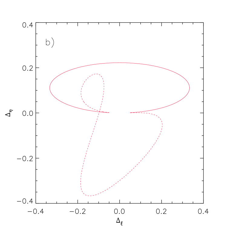
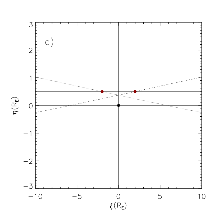
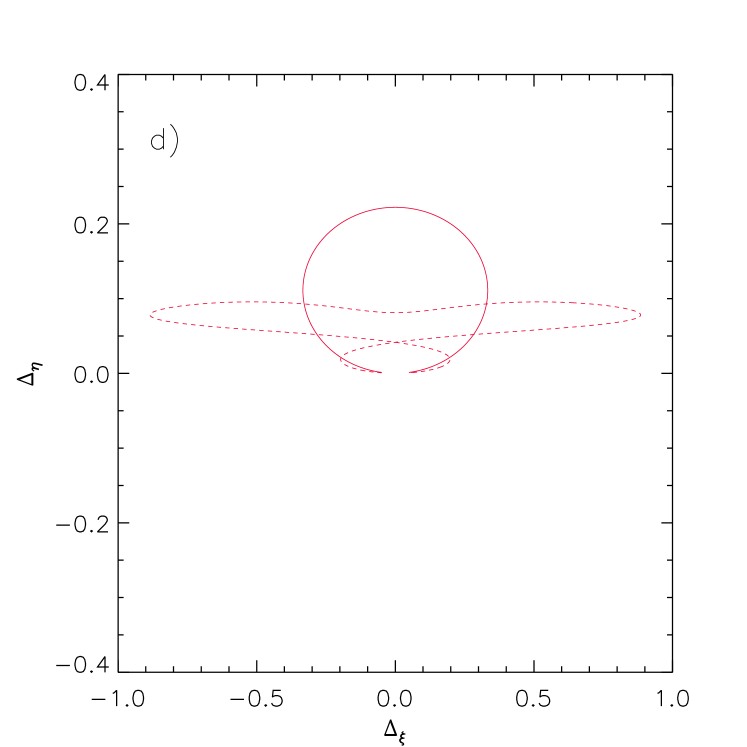
Figure 1: We give the source path (left panels) and the corresponding astrometric curves (right panels) for a binary source with components of mass $m_{1}=m_{2}=1$ M_⊙, with the same luminosity, and separated by $10$ AU. The lens has a mass of $m_{l}=1$ M_⊙, is located at $D_{L}=1$ kpc and moves with a projected velocity $v_{\perp}=100$ km s^-1, thus implying an Einstein angular radius of $2.7$ mas. The event impact parameter is $u_{0}=0.5$. The upper panels show the expected signal for a static binary source, while in the bottom ones the orbital motion is taken into account. For the simulated event, the Einstein time and the binary source orbital period are $t_{E}\simeq 46$ days and $P\simeq 8674$ days, respectively. In the right panels the continuous ellipses represent the astrometric trajectories for a single source located in the center of mass, while dashed lines stand for the binary source.

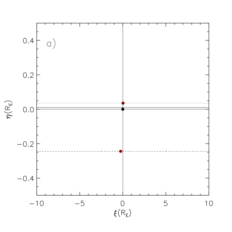
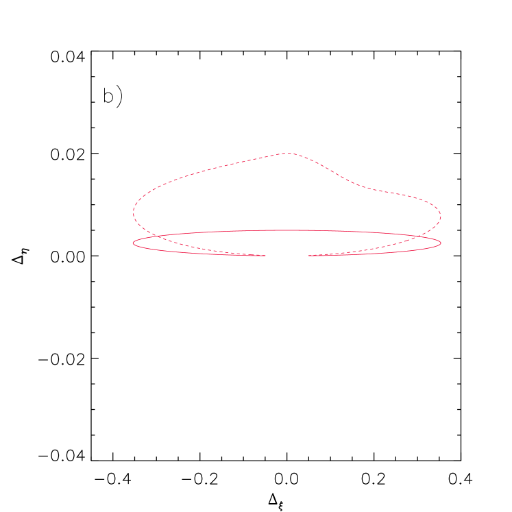
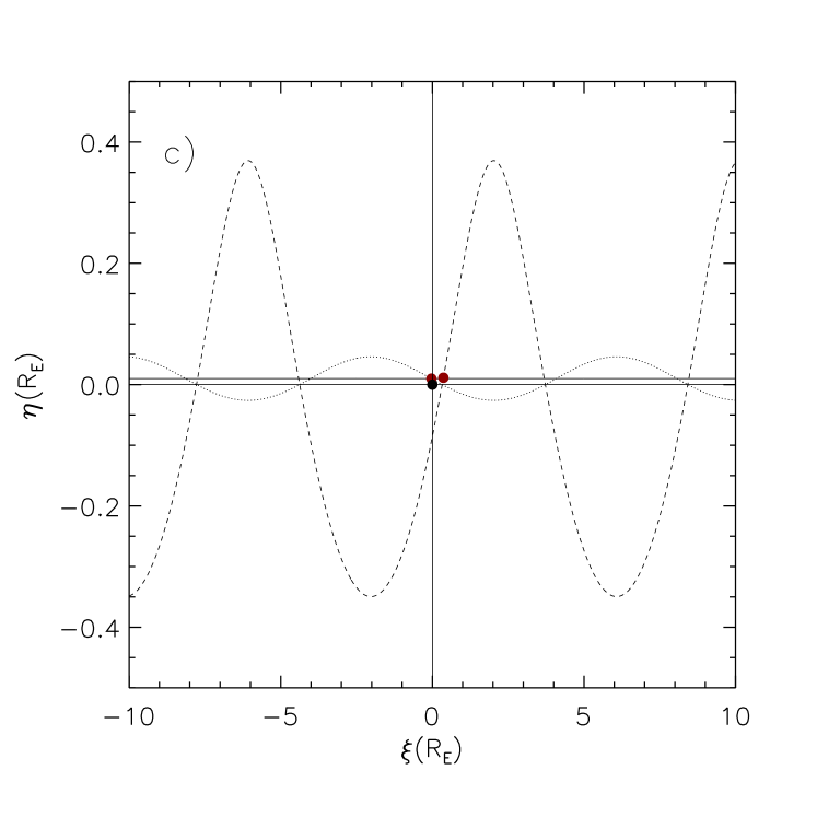
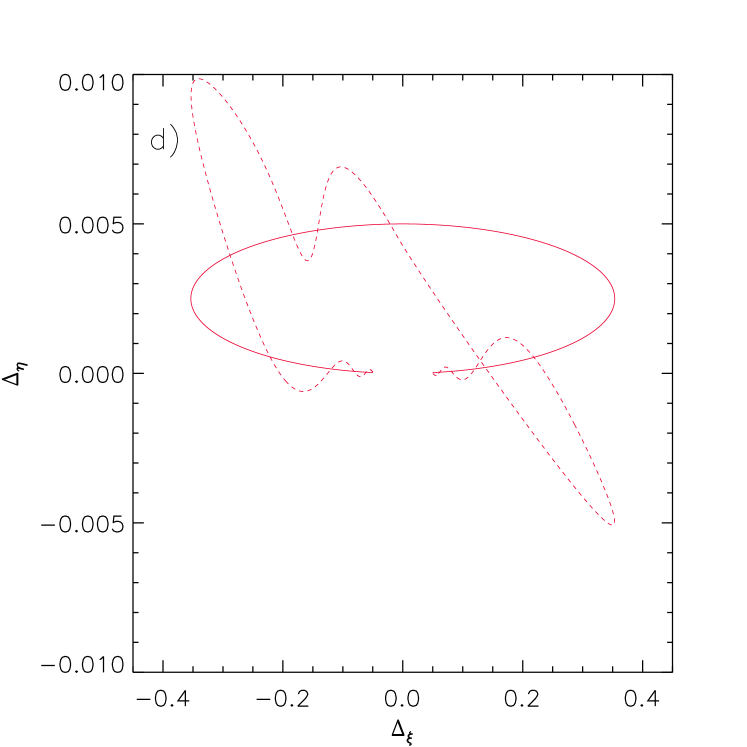
Figure 2: The same as in Figure 1, for a binary source with components of mass $m_{1}=1$ M_⊙, $m_{2}=0.1$ M_⊙, $F_{1}=1$, $F_{2}=10^{-2}$, and separated by $1$ AU. The lens has a mass of $m_{l}=1$ M_⊙, is located at $D_{L}=1$ kpc and moves with a projected velocity $v_{\perp}=100$ km s^-1, thus implying an Einstein angular radius of $2.7$ mas. The event impact parameter is $u_{0}=0.01$. For the simulated event, the Einstein time and the binary source orbital period are $\simeq 46$ days and $\simeq 369$ days, respectively.

In both Figures, the solid curves represent the centroid shift ellipse expected for a single source located at the center of mass of the binary source system. It is evident that the presence of a binary source system introduces deformations of the astrometric signal with respect to the pure ellipse case. This is also true when the orbital motion of the binary source system is taken into account as illustrated in the lower panels of Figures 1 and 2, where modulations with a time scale corresponding to the source system orbital period do appear.

Note that, for the considered cases, being $\theta_{E}\simeq 2.7$ mas, the astrometric signal results well within the astrometric precision of the Gaia satellite in five years of integration. This opens the possibility to detect binary systems as sources of astrometric microlensing events and characterize their physical parameters (mass ratio, projected separation and orbital period).

We would like to mention the challenging possibility for Gaia-like observatories to detect also astrometric microlensing events involving both binary sources and binary lenses. For the sake of simplicity, we do not consider here the orbital motion of the systems. For such cases, eq. (22) remains valid provided that the centroid shifts ${\rm\Delta_{i}}$ of each components of the binary source system are obtained solving numerically the two body lens equation. In this case the lens equation is expressed as (Witt 1990; Witt & Mao 1995; Skowron & Gould 2012),

$$\zeta_{i}=z_{i}+\frac{m_{L,1}}{z_{L,1}+\bar{z}_{i}}+\frac{m_{L,2}}{z_{L,2}+\bar{z}_{i}},$$ (25)

where $m_{L,1}$ and $m_{L,2}$ are the masses of the binary lens components (with $m_{L,2}<m_{L,1}$ so that $q_{L}=m_{L,2}/m_{L,1}<1$ ), $z_{L,1}$ and $z_{L,2}$ the positions of the lenses (separated by $b_{L}$), and $\zeta_{i}=\xi_{i}+i\eta_{i}$ and $z_{i}=x_{i}+iy_{i}$ the positions of the binary source components and associated images, respectively. The lens components are located on the $\xi$ axis with the primary at $(-b_{L}/2,0)$ and secondary at $(b_{L}/2,0)$.

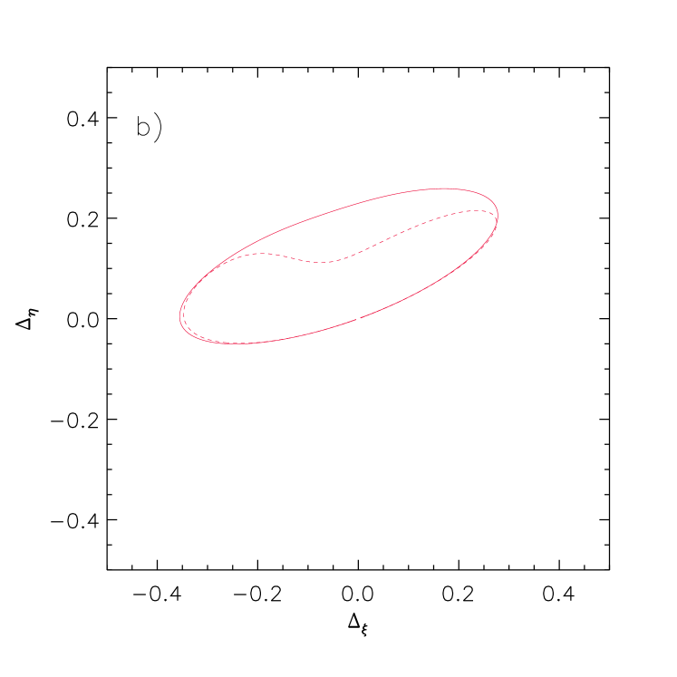
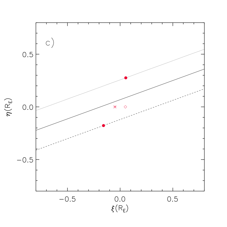
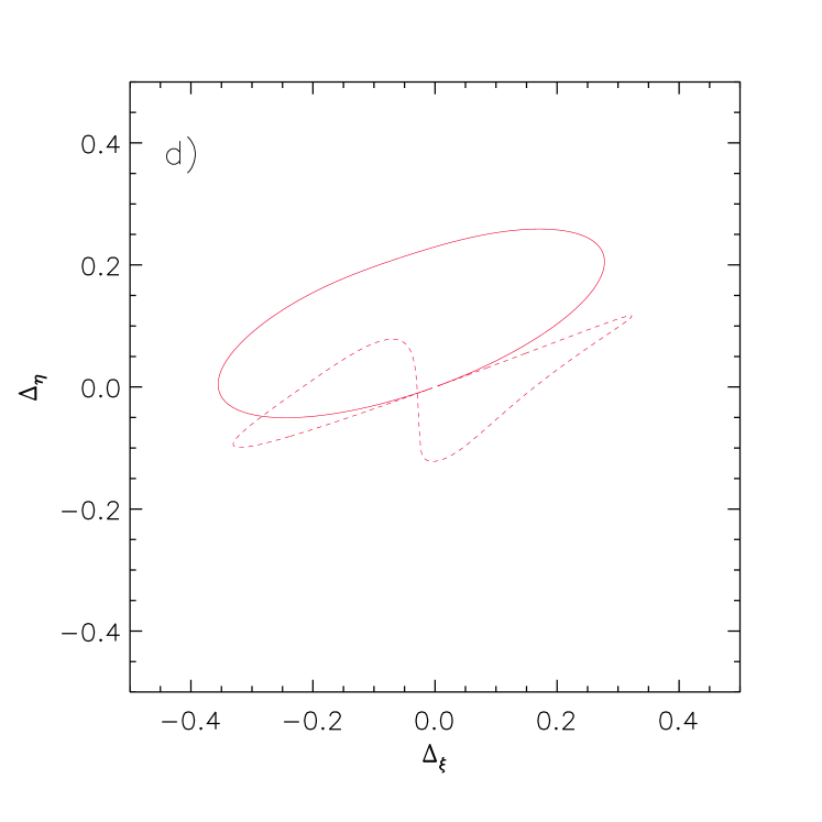
Figure 3: We give the source path (left panels) for the primary source (dotted line), its companion (dashed line), and the associated center of mass (solid line). The asterisk and diamond represent the location of the primary and secondary lens, resepctively. The expected astrometric signal is given in the right panels for a binary source ($b=0.5$, $q=1$) lensed by a binary lens ($b=q=0.1$) with impact parameter $u_{0}=0.5$ (panel b) and impact paremeter $u_{0}=0.05$ (panel d).

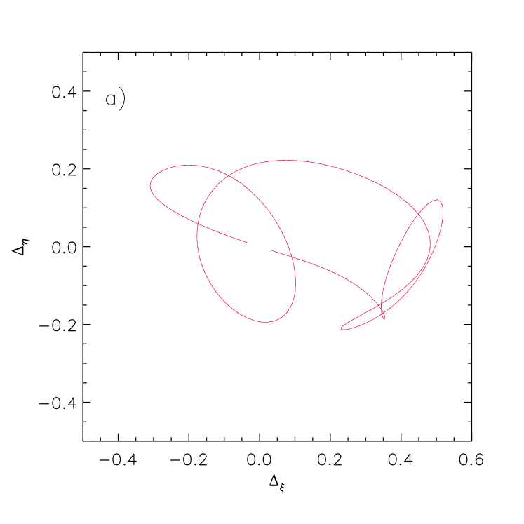
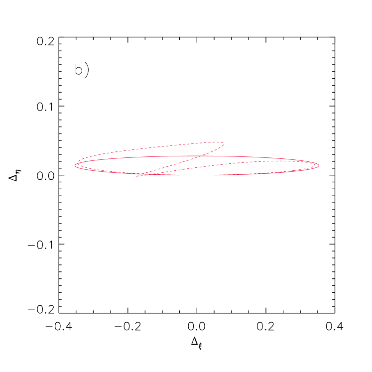
Figure 4: For the event OGLE 2002-BLG-099, we give the simulated astrometric path for the binary lens and single source (left panel for $q=0.248$, $b=1.963$, $u_{0}=0.09$, and $t_{E}=24.4$ days) and for the single lens and binary source (right panel for $u_{0,1}=0.0821$, $u_{0,2}=0.0294$, corresponding to peak times of $t_{0,1}=2402.93$ days and $t_{0,2}=2425.23$, $t_{E}=47.1$ days, and blending parameters $f_{1}=0.147$ and $f_{2}=0.051$) cases, respectively.

In this case, the centroid shifts with respect to the position of the unlensed star (one per each of the intervening source, see also Han 2001) are

$$(\Delta_{\xi,i},\Delta_{\eta,i})=(x_{c,i}-\xi_{i},y_{c,i}-\eta_{i}),$$ (26)

where the positions of the source star centroid are simply the average of the locations of the individual images wighted by each corresponding amplification $\mu_{j,i}$, i.e.

$$(x_{c,i},y_{c,i})=\left(\sum_{j}\mu_{j,i}x_{i}/\mu_{i},\sum_{j}\mu_{j,i}y_{i}/\mu_{i}\right).$$ (27)

Here, $\mu_{i}$ is the total amplification (i.e. $\mu_{i}=\sum_{j}\mu_{j,i}$, with $j$ running over the image number) and, as above, $i=1,2$ indicates the primary and secondary component of the binary source system. As an example, in panel (a) of Figure 3, we present the paths of the primary (dotted line), and secondary (dashed line) components of the binary source system characterized by $b=0.5$, and $q=1$. The solid line indicates the path followed by the center of mass. The binary source system (assumed here for simplicity to be static) is lensed by a binary lens with $b_{L}=q_{L}=0.1$ and the event impact parameter is $u_{0}=0.5$. The asterisk and diamond represent the position of the primary and secondary lenses, respectively. In panel (b) we give the astrometric signal (dashed line) expected for the simulated microlensing event. For comparison, the solid line represents the astrometric signal associated to the same binary lens acting on a single point-like source. Note that the presence of a binary source gives a substantial difference with respect to the single source case that, for the assumed simulated event parameters, amounts to $\simeq 0.1\theta_{E}\simeq 270$ $\mu$as, well within the Gaia capabilities. In panels (c) and (d), we set the event impact parameter to $u_{0}=0.05$, leaving the other parameters unchanged. In this case the astrometric signal is completely different with respect to the previous case. This is a general behaviour of the astrometric shift curves which strongly depend even to small changes of the system physical parameters. It goes without saying that, conversely to what happens with the standard photometric microlensing, a fitting procedure on the observed astrometric data may provide a robust estimate of the microlensing event parameters. This is clear when considering events not well sampled as OGLE 2002-BLG-099 (see Jaroszyński et al. 2004 for details) where different interpretations of the photometric data are statistically acceptable. In particular, the considered event can be described as due to a single source lensed by a binary system or by a double source lensed by a single object. While the light curve analysis does not allow one to distinguish between these models, it is clear from Fig. 4, that astrometric observations would have resolved the degeneracy since the astrometric signals associated to the two cases are completely different. Indeed, considering the most likely values for the total lens mass and distance of $\simeq 0.47$ M_⊙ and $D_{L}\simeq 5.7$ kpc (Dominik 2006) one gets $\theta_{E}\simeq 470$ $\mu$as. Hence, from Fig. 4, astrometric observations with precision of at least $40-50$ $\mu$as (i.e. within the capabilities of the Gaia satellite) would make possible the distinction between the two different configurations.

4 Earth parallax effects on astrometric microlensing

In photometric observation of microlensing events the parallax effect, due to the Earth motion, generally induces minor anomalies unless the event Einstein time is comparable with (or longer than) the Earth orbital period (see, e.g., Wyrzykowski et al. 2016). On the contrary, in astrometric microlensing the Earth orbital motion is not negligible even for short duration events. Here, based on the seminal idea by Paczyński (1998) we account for the parallax effect following

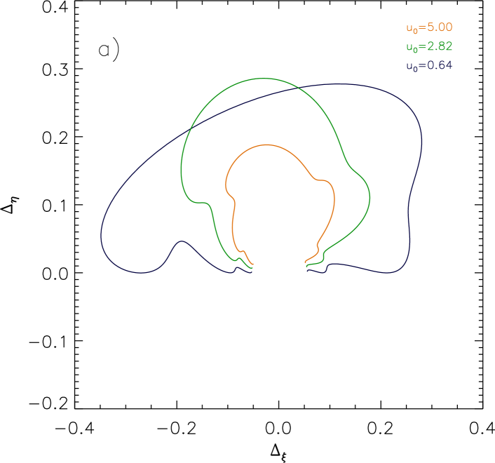
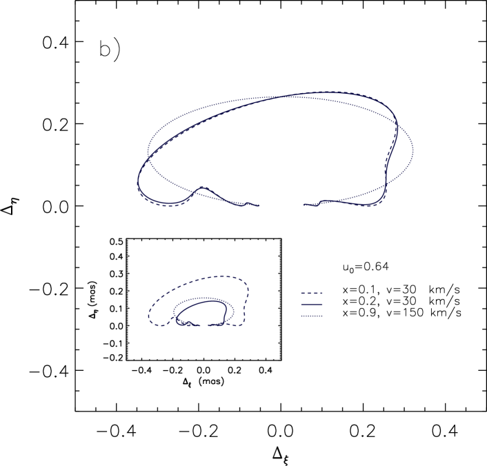
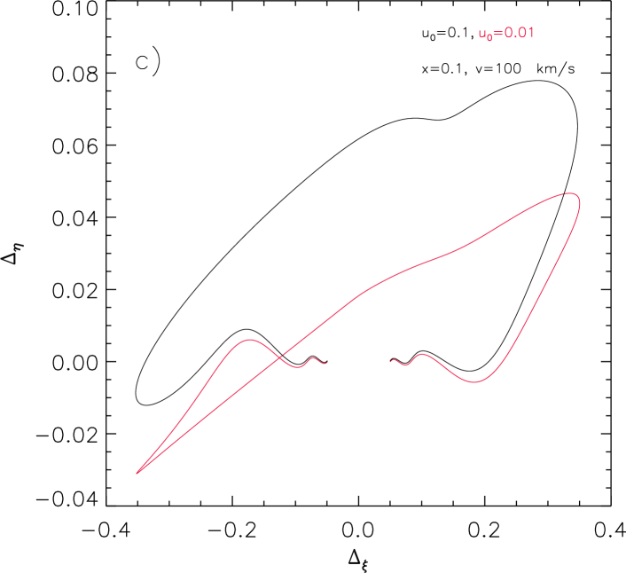
Figure 5: Earth parallax effect on astrometric curves for three simulated microlensing events (see text for details).

the formalism provided by Dominik (1998 a) in the approximation of small orbital eccentricity. Let $\xi_{0}(t)$ and $\eta_{0}(t)$ be the coordinates of the source (not corrected for parallax effect) in the lens plane at time $t$. The new coordinates are

$$\begin{split}\xi(t)&=\xi_{0}(t)+(\tilde{x}_{1}(t)-\tilde{x}_{1}(t_{0}))\cos\psi\\ &\quad{}+(\tilde{x}_{2}(t)-\tilde{x}_{2}(t_{0}))\sin\psi,\end{split}$$ (28a)

$$\begin{split}\eta(t)&=\eta_{0}(t)-(\tilde{x}_{1}(t)-\tilde{x}_{1}(t_{0}))\sin\psi\\ &\quad{}+(\tilde{x}_{2}(t)-\tilde{x}_{2}(t_{0}))\sin\psi,\end{split}$$ (28b)

where

$$\tilde{x}_{1}(t) =-A^{\prime}(t)\sin\chi\cos\nu(t),$$ (29a)

$$\tilde{x}_{2}(t) =A^{\prime}(t)\sin\nu(t),$$ (29b)

$$A^{\prime}(t) =a_{\oplus}\bigl{[}1-\varepsilon_{\oplus}\cos M(t)\bigr{]}\frac{1-x}{R_{\textup{E}}},$$ (29c)

$$\nu(t) =M(t)+2\varepsilon_{\oplus}\sin M(t)-\varphi,$$ (29d)

$$M(t) =2\pi\frac{t-t_{\textup{p}}}{P_{\oplus}},$$ (29e)

$$x =D_{\textup{L}}/D_{\textup{S}}.$$ (29f)

In the previous equations, $M(t)$ is the mean anomaly of the Earth, $t_{\textup{p}}$ is the last time of perihelion passage, so that $M$ lies in the interval $[0,2\pi[$ , $\nu(t)$ its true anomaly shifted by $\varphi$. In addition, $\varphi$ and $\chi$ are, respectively, the longitude and the latitude of the source measured in the ecliptic plane as prescribed by Dominik (1998 a), while $\psi$ is the relative orientation of $\boldsymbol{v}_{\perp}$ to the Sun-Earth system. Here, $a_{\oplus}\simeq 1.49\times 10^{13}~{}\textup{cm}$ is the Earth orbit semi-major axis, $\varepsilon_{\oplus}=0.0167$ is its eccentricity, and $P_{\oplus}=365.26~{}\textup{d}$ the orbital period. In the definition of $A^{\prime}(t)$, note that $\rho^{\prime}=a_{\oplus}(1-x)/R_{\textup{E}}$ is the Earth semi-major axis projected onto the lens plane, in units of Einstein radii, and is a measure of the importance of parallax effect.

In Figure 5, we show the astrometric curves (obtained with an integration time of $\simeq 5$ years) for three simulated events taking into account the Earth parallax and assuming $t_{0}=t_{p}=0$. In all cases, we fixed the source coordinates to be $\varphi=2.93$ rad, and $\chi=-0.08$ rad as in Dominik (1998 a) cooresponding to ecliptic coordinates $\lambda=271^{\circ}$, and $\beta=-5^{\circ}$.

In the upper panel, a single source is microlensed by a single lens ($x=0.1$, $v=30$ km s^-1 and $t_{E}=50$ days corresponding to $\theta_{E}\simeq 1$ mas) for three different impact parameters. In the middle panel, we fixed the impact parameter to $u_{0}=0.64$ leaving the other parameters unchanged. Dashed and continuous curves are for two disk events at different distances from the observer, $x=0.1$ and $x=0.2$ (corresponding to $\theta_{E}\simeq 1$ mas and $\theta_{E}\simeq 0.5$ mas), respectively. The dotted line has been obtained for a bulge lens ($x=0.9$) with $\theta_{E}\simeq 0.6$ mas. The inset shows the scaled astrometric signal in physical units. Finally, in the bottom panel, we give the expected astrometric signal (red curve) for a (static) binary source microlensed by a single object, assuming the same parameters as in Figure 2 and $u_{0}=0.01$. The black line corresponds to an event with impact parameter $u_{0}=0.1$. In both cases, $x=0.1$, $\theta_{E}\simeq 2.5$ mas and $t_{E}=45.6$ days.

It is worth mentioning that while in standard photometric microlensing the parallax effect becomes more important close to the event peak and (especially) for long events, in astrometric observations the deviations with respect to the pure ellipse path show up even in the case of events characterized by short $t_{E}$. Moreover, modulations with the Earth orbital period appear, also at very large impact parameter values where the photometric signal is useless. As a final note, we remark that taking into account the source orbital motion produces modulations with a peculiar frequency characteristic of the system.

5 Conclusions

In this paper we considered the anomalies induced in simulated astrometric events by the orbital motion of the lens and/or source binary systems taking into account the Earth parallax effect. Considering and implementing these effects in astrometric microlensing is essential in order to correctly estimate the system parameters thus alleviating the parameter degeneracy problem that afflicts photometric microlensing. This issue is particularly important in the era of Gaia satellite that is performing a survey of the whole sky allowing one to get the astrometric path of microlensed sources with unprecedent precision. Indeed, it has been estimated that the Gaia mission will discover, in five years of operations, $\simeq 3500$ photometric and $25000$ astrometric microlensing events (Belokurov & Evans 2002) which will be characterized by a astrometric precision down to 30 $\mu$as. An even better precision could be possibly obtained by following up the events discovered by Gaia with ground-based observations (as Gravity at VLT, see Eisenhauer et al. 2009 but also Zurlo et al. 2014) for a longer observation time. This is important since the astrometric path of microlensing event changes substantially during a much longer time interval than in the usual photometric observations.

References

- Belokurov & Evans (2002) Belokurov V.A., & Evans N.W., 2002, MNRAS, 331, 649
- Bennett et al. (2015) Bennett D.P., et al., 2015, ApJ, 808, 169
- Bozza (2001) Bozza V., 2001, A&A, 374, 13
- Dalal & Griest (2001) Dalal N, & Griest K., 2001, ApJ, 561, 481
- Dominik (1997) Dominik M., 1997, Galactic Microlensing Beyond The Standard Model, Ph.D. Thesis at University of Dortmund.
- Dominik (1998 a) Dominik, M., 1998 a, A&A, 329, 361
- Dominik (1998 b) Dominik, M., 1998 b, A&A, 333, 893
- Dominik & Sahu (2000) Dominik M., & Sahu K., 2000, ApJ, 534, 213
- Dominik (2006) Dominik M., 2006, MNRAS, 367, 669
- Eisenhauer et al. (2009) Eisenhauer F., et al., 2009, in Science with the VLT in the ELT Era ASS Proceedings, ISBN 978-1-4020-9189-6. Springer Netherlands, p. 361
- Eyer et al. (2013) Eyer L., Holl B., Pourbaix D., et al., 2013, CEAB, 37, L115
- Giordano et al. (2015) Giordano M., Nucita A.A., De Paolis F., & Ingrosso G., 2015, MNRAS, 453, 2017
- Griest & Hu (1992) Griest K., & Hu W, 1992, ApJ, 397, 362 (Erratum: 1993, ApJ, 407, 440)
- Han (2001) Han C., 2001, MNRAS, 328, 611
- Han et al. (1999) Han C., Chun M., & Chang K., 1999, ApJ 526, 405
- Han et al. (2001) Han C., Chun M., & Chang K., 2001, MNRAS, 328, 986
- Han & Kim (1999) Han C., Kim T.-W., 1999, MNRAS, 305, 795
- Hideki (2002) Hideki A., 2002, ApJ, 573, 825A
- Høg et al. (1995) Høg E., Novikov I. D., & Polnarev A. G,. 1995, A & A, 294, L287
- Hwang et al. (2013) Hwang K.-H., et al., 2013, ApJ, 778, 55
- Ingrosso et al. (2014) Ingrosso G., et al., 2014, Phys. Scripta, 89, ID 084001
- Ingrosso et al. (2015) Ingrosso G., et al., 2015, MNRAS, 446, 1090
- Jaroszyński et al. (2004) Jaroszyński M., et al., 2004, Acta. Astron, 54, 103
- Jeong et al. (1995) Jeong Y., Han C., & Park S.-H., 1999, ApJ, 511, L569
- Lee et al. (2010) Lee C.-H., Seitz S., Riffeser A., & Bender R., 2010, MNRAS, 407, 1597
- Luhn et al. (2015) Luhn, J. K., Penny, M. T. & Gaudi, B. S., 2015, eprint arXiv:1510.08521
- Miyamoto & Yoshii (1995) Miyamoto M. & Yoshii Y., 1995, AJ, 110, 1427
- Nucita et al. (2014) Nucita A.A., Giordano M., De Paolis F., & Ingrosso G., 2014, MNRAS, 438, 2466
- Paczyński (1986) Paczyńsky B., 1986, ApJ, 304, 1
- Paczyński (1995) Paczyńsky B., 1995, Acta. Astron, 45, 345
- Paczyński (1996) Paczyński B., 1996, Acta Astron., 46, L291.
- Paczyński (1998) Paczyński B., 1998, ApJ, 494, L23.
- Park et al. (2015) Park H., at al., 2015, ApJ, 805, 117P
- Penny et al. (2011 a) Penny M.T., Mao S., & Kerins E., 2011, MNRAS, 412, 607.
- Penny et al. (2011 b) Penny M.T., Kerins E., & Mao S., 2011, MNRAS, 417, 2216
- Proft et al. (2011) Proft S., Demleitner M., & Wambsganss J., 2011, A&A, 536, A50
- Safizadeh et al. (1999) Safizadeh N., Dalal N., & Griest K., 1999, ApJ, 522, 512S
- Sajadian & Rahvar (2015) Sajadian S., & Rahvar S., 2015, MNRAS, 452, 2579
- Schneider, Ehlers & Falco (1992) Schneider P., Ehlers J., & Falco E.E., 1992, Gravitational Lenses, New York, Springer
- Skowron & Gould (2012) Skowron, J., & Gould, A. 2012, eprint arXiv:1203.1034
- Skowron et al. (2015) Skowron J., et al., 2015, ApJ, 804, 33S
- Takahashi (2003) Takahaschi R., 2003, ApJ, 595, 418
- Udalski et al. (2015) Udalski U., et al., 2015, ApJ, 812, 47
- Walker (1995) Walker M., A., 1995, ApJ, 453, 37
- Witt (1990) Witt H.-J., 1990, A&A, 236, 311
- Witt & Mao (1995) Witt H.-J., & Mao S., 1995, ApJ, 447, L105
- Wyrzykowski et al. (2016) Wyrzykowski L., et al., 2016, MNRAS, in press
- Zurlo et al. (2014) Zurlo A., et al., A&A 2014, 572, 85