Three Notes on Ser’s and Hasse’s Representations
for the Zeta-Functions
Iaroslav V. Blagouchine
SeaTech, University of Toulon, France.
St. Petersburg State University of Architecture and Civil Engineering, Russia.
iaroslav.blagouchine@univ-tln.fr, iaroslav.blagouchine@pdmi.ras.ru

Abstract

This paper is devoted to Ser’s and Hasse’s series representations for the zeta-functions, as well as to several closely related results. The notes concerning Ser’s and Hasse’s representations are given as theorems, while the related expansions are given either as separate theorems or as formulæ inside the remarks and corollaries. In the first theorem, we show that the famous Hasse’s series for the zeta-function, obtained in 1930 and named after the German mathematician Helmut Hasse, is equivalent to an earlier expression given by a little-known French mathematician Joseph Ser in 1926. In the second theorem, we derive a similar series representation for the zeta-function involving the Cauchy numbers of the second kind (Nørlund numbers). In the third theorem, with the aid of some special polynomials, we generalize the previous results to the Hurwitz zeta-function. In the fourth theorem, we obtain a similar series with Gregory’s coefficients of higher order, which may also be regarded as a functional equation for the zeta-functions. In the fifth theorem, we extend the results of the third theorem to a class of Dirichlet series. As a consequence, we obtain several globally convergent series for the zeta-functions. They are complementary to Hasse’s series, contain the same finite differences and also generalize Ser’s results. In the paper, we also show that Hasse’s series may be obtained much more easily by using the theory of finite differences, and we demonstrate that there exist numerous series of the same nature. In the sixth theorem, we show that Hasse’s series is a simple particular case of a more general class of series involving the Stirling numbers of the first kind. All the expansions derived in the paper lead, in turn, to the series expansions for the Stieltjes constants, including new series with rational terms only for Euler’s constant, for the Maclaurin coefficients of the regularized Hurwitz zeta-function, for the logarithm of the gamma-function, for the digamma and trigamma functions. Throughout the paper, we also mention several “unpublished” contributions of Charles Hermite, which were very close to the results of Hasse and Ser. Finally, in the Appendix, we prove an interesting integral representation for the Bernoulli polynomials of the second kind, formerly known as the Fontana–Bessel polynomials.

1 Introduction

The Euler–Riemann zeta-function

$$\,\zeta(s)\equiv\sum\limits_{n=1}^{\infty}n^{-s}\,=\prod\limits_{n=1}^{\infty}\!\big{(}1-p_{n}^{-s}\big{)}^{-1}\,\,,\qquad\begin{array}[]{l}\mathop{\rm Re}\nolimits s>1\\[2.84526pt] p_{n}\in\mathbbm{P}\,,\end{array}$$

and its most common generalization, the Hurwitz zeta-function

$$\,\zeta(s,v)\equiv\sum\limits_{n=0}^{\infty}(n+v)^{-s}\,,\qquad\begin{array}[]{l}\mathop{\rm Re}\nolimits s>1\\[2.84526pt] v\in\mathbbm{C}\setminus\!\{0,-1,-2,\ldots\}\,,\end{array}$$

$\zeta(s)=\zeta(s,1)$, are some of the most important special functions in analysis and number theory. They were studied by many famous mathematicians, including Stirling, Euler, Malmsten, Clausen, Kinkelin, Riemann, Hurwitz, Lerch, Landau, and continue to receive considerable attention from modern researchers. In 1930, the German mathematician Helmut Hasse published a paper [37], in which he obtained and studied these globally convergent series for the $\zeta$–functions

$$\zeta(s)\,=\,\frac{1}{\,s-1\,}\sum_{n=0}^{\infty}\frac{1}{\,n+1\,}\sum_{k=0}^{n}(-1)^{k}\binom{n}{k}(k+1)^{1-s}\,,$$ (1)

$$\zeta(s,v)\,=\,\frac{1}{\,s-1\,}\sum_{n=0}^{\infty}\frac{1}{\,n+1\,}\sum_{k=0}^{n}(-1)^{k}\binom{n}{k}(k+v)^{1-s}\,,$$ (2)

containing finite differences $\,\Delta^{n}1^{1-s}\,$ and $\,\Delta^{n}v^{1-s}\,$ respectively. Hasse also remarked that the first series is quite similar to the Euler transformation of the $\eta$-function series $\,\eta(s)\equiv\sum\limits_{n=1}^{\infty}(-1)^{n+1}n^{-s}=\big{(}1-2^{1-s}\big{)}\,\zeta(s)\,$, $\,\mathop{\rm Re}\nolimits s>0\,$, i.e.

$$\zeta(s)\,=\,\frac{1}{\,1-2^{1-s}\,}\sum_{n=0}^{\infty}\frac{1}{\,2^{n+1}\,}\sum_{k=0}^{n}(-1)^{k}\binom{n}{k}(k+1)^{-s}\,,$$ (3)

the expression which, by the way, was earlier given by Mathias Lerch [48] and later rediscovered by Jonathan Sondow [69], [26]. Formulæ (1)–(2) have become widely known, and in the literature they are often referred to as Hasse’s formulæ for the $\zeta$-functions. At the same time, it is not so well known that 4 years earlier, a little-known French mathematician Joseph Ser published a paper [65] containing very similar results. In particular, he showed that

$$\zeta(s)\!\! =\,\frac{1}{\,s-1\,}\sum_{n=0}^{\infty}\frac{1}{\,n+2\,}\sum_{k=0}^{n}(-1)^{k}\binom{n}{k}(k+1)^{-s},$$ (4)

and also gave this curious series

$$\zeta(s)\!\! =\,\frac{1}{\,s-1\,}+\sum_{n=0}^{\infty}\big{|}G_{n+1}\big{|}\sum_{k=0}^{n}(-1)^{k}\binom{n}{k}(k+1)^{-s}\,=$$

$$=\,\frac{1}{\,s-1\,}+\frac{1}{2}+\frac{1}{12}\big{(}1-2^{-s}\big{)}+\frac{1}{24}\big{(}1-2\cdot 2^{-s}+3^{-s}\big{)}+\ldots$$

[65, Eq. (4), p. 1076], [9, p. 382], to which Charles Hermite was also very close already in 1900. The numbers $G_{n}$ appearing in the latter expansion are known as Gregory’s coefficients and may also be called by some authors (reciprocal) logarithmic numbers, Bernoulli numbers of the second kind, normalized generalized Bernoulli numbers $B_{n}^{(n-1)}$ and $B_{n}^{(n)}(1)$, and normalized Cauchy numbers of the first kind $C_{1,n}$. They are rational and may be defined either via their generating function

$$\frac{z}{\ln(1+z)}\,=\,1\,+\sum_{n=1}^{\infty}G_{n}\,z^{n},\qquad|z|<1\,,$$ (6)

or explicitly via the recurrence relation

$$G_{n}\,=\,\frac{(-1)^{n-1}}{\,n+1\,}\,+\sum_{k=1}^{n-1}\!\frac{(-1)^{n+1-k}G_{k}}{\,n+1-k\,}\,,\qquad G_{1}=\frac{1}{2}\,,\quad n=2,3,4,\ldots$$ (7)

see e.g. [68, p. 10], [6], [54, pp. 261–262, § 61], [44, p. 143], [45, p. 423, Eq. (30)], or via

$$G_{n} =\,\frac{C_{1,n}}{n!}\,=-\frac{B_{n}^{(n-1)}}{\,(n-1)\,n!\,}=\frac{B^{(n)}_{n}(1)}{n!}\,=\int\limits_{0}^{1}\!\!\binom{x}{n}\,dx\,$$ (8)

$$=\,\frac{1}{n!}\!\int\limits_{0}^{1}\!(x-n+1)_{n}\,dx\,=\,\frac{1}{n!}\!\sum\limits_{l=1}^{n}\frac{S_{1}(n,l)}{l+1}\,,$$

where $n$ is a natural number, $\,(x)_{n}\equiv\,x\,(x+1)\,(x+2)\cdots(x+n-1)\,$ stands for the Pochhammer symbol (also known as the rising factorial) and $S_{1}(n,l)$ are the Stirling numbers of the first kind, which are the coefficients in the expansion of the falling factorial, and hence of the binomial coeffcient,

$$(x-n+1)_{n}=\,n!\binom{x}{n}=\,x\,(x-1)\,(x-2)\cdots(x-n+1)\,=\,\sum_{l=1}^{n}S_{1}(n,l)\,x^{l}.$$ (9)

Gregory’s coefficients are alternating $\,G_{n}=(-1)^{n-1}|G_{n}|\,$ and decreasing in absolute value; they behave as $\,\big{(}n\ln^{2}n\big{)}^{-1}$ at $n\to\infty$ and may be bounded from below and from above accordingly to formulæ (55)–(56) from [10]. The first few coefficients are: $G_{1}=+\nicefrac{{1}}{{2}}\,$, $G_{2}=\nicefrac{{-1}}{{12}}\,$, $G_{3}=\nicefrac{{+1}}{{24}}\,$, $G_{4}=\nicefrac{{-19}}{{720}}\,$, $G_{5}=\nicefrac{{+3}}{{160}}\,$, $G_{6}=\nicefrac{{-863}}{{60\,480}}\,$,… For more information about these important numbers, see [10, pp. 410–415], [9, p. 379], and the literature given therein (nearly 50 references).

2 On the equivalence between Ser’s and Hasse’s representations for the Euler–Riemann zeta-function

One may immediately see that Hasse’s representation (1) and Ser’s representation (4) are very similar, so one may question whether these expressions are equivalent or not. The paper written by Ser [65] is much less cited than that by Hasse [37], and in the few works in which both of them are cited, these series are treated as different and with no connection between them. However, as we shall show later, this is not true.

In one of our previous works [9, p. 382], we already noticed that these two series are, in fact, equivalent, but this was stated in a footnote and without a proof. Below, we provide a rigorous proof of this statement.

Theorem 1.

Ser’s representation for the $\zeta$-function [65, p. 1076, Eq. (7)]

$$\zeta(s)\,=\,\frac{1}{\,s-1\,}\sum_{n=0}^{\infty}\frac{1}{\,n+2\,}\sum_{k=0}^{n}(-1)^{k}\binom{n}{k}(k+1)^{-s}\,,\qquad s\in\mathbbm{C}\setminus\!\{1\}\,,$$ (10)

and Hasse’s representation for the $\zeta$-function [37, pp. 460–461]

$$\zeta(s)\,=\,\frac{1}{\,s-1\,}\sum_{n=0}^{\infty}\frac{1}{\,n+1\,}\sum_{k=0}^{n}(-1)^{k}\binom{n}{k}(k+1)^{1-s}\,,\qquad s\in\mathbbm{C}\setminus\!\{1\}\,,$$ (11)

are equivalent in the sense that one series is a rearranged version of the other.

Proof.

In view of the fact that

$$\frac{1}{\,k+1\,}\binom{n}{k}=\frac{1}{\,n+1\,}\binom{n+1}{k+1}\quad\text{and that}\quad\frac{1}{\,(n+2)(n+1)\,}=\frac{1}{\,n+1\,}-\frac{1}{\,n+2\,}\,,$$

Ser’s formula (10), multiplied by the factor $s-1$, may be written as:

$$\left(s-1\right)\zeta(s)\!\!\! \,=\sum_{n=0}^{\infty}\frac{1}{\,n+2\,}\sum_{k=0}^{n}(-1)^{k}\binom{n}{k}(k+1)^{-s}$$

$$=\sum_{n=0}^{\infty}\frac{1}{\,(n+2)(n+1)\,}\sum_{k=0}^{n}(-1)^{k}\binom{n+1}{k+1}(k+1)^{1-s}$$

$$=\sum_{n=0}^{\infty}\frac{1}{\,n+1\,}\sum_{k=0}^{n}(-1)^{k}\binom{n+1}{k+1}(k+1)^{1-s}-$$

$$\qquad\qquad-\sum_{n=0}^{\infty}\frac{1}{\,n+2\,}\sum_{k=0}^{n}(-1)^{k}\binom{n+1}{k+1}(k+1)^{1-s}=$$

$$=1+\sum_{n=1}^{\infty}\frac{1}{\,n+1\,}\sum_{k=0}^{n}(-1)^{k}\binom{n+1}{k+1}(k+1)^{1-s}-$$

$$\qquad\qquad-\sum_{n=1}^{\infty}\frac{1}{\,n+1\,}\sum_{k=0}^{n-1}(-1)^{k}\binom{n}{k+1}(k+1)^{1-s}=$$

$$=1+\sum_{n=1}^{\infty}\frac{(-1)^{n}}{\,(n+1)^{s}\,}+\sum_{n=1}^{\infty}\frac{1}{\,n+1\,}\sum_{k=0}^{n-1}\frac{(-1)^{k}}{(k+1)^{s-1}}\left\{\!\binom{n+1}{k+1}-\binom{n}{k+1}\!\right\}$$

$$\,=\,1+\sum_{n=1}^{\infty}\frac{(-1)^{n}}{\,(n+1)^{s}\,}+\,\sum_{n=1}^{\infty}\frac{1}{\,n+1\,}\sum_{k=0}^{n-1}\frac{(-1)^{k}}{(k+1)^{s-1}}\binom{n}{k}$$

$$\,=\,1+\sum_{n=1}^{\infty}\frac{1}{\,n+1\,}\sum_{k=0}^{n}\frac{(-1)^{k}}{(k+1)^{s-1}}\binom{n}{k}\,=\sum_{n=0}^{\infty}\frac{1}{\,n+1\,}\sum_{k=0}^{n}\frac{(-1)^{k}}{(k+1)^{s-1}}\binom{n}{k}\,,$$

where, between the seventh and eighth lines, we resorted to the recurrence relation for the binomial coefficients. The last line is identical with Hasse’s formula (11). ∎

Thus, series (10) and (11) are equivalent in the sense that (11) may be obtained by an appropriate rearrangement of terms in (10) and vice versa. It is also interesting that Hasse’s series for $\zeta(s)$ may be obtained from that for $\zeta(s,v)$ by simply setting $v=1$, while Ser’s series for $\zeta(s)$, as we come to see later, is obtained from a much more complicated formula for $\zeta(s,v)$, see (129)–(128) hereafter.

Corollary 1.

The Stieltjes constants $\gamma_{m}$ may be given by the following series

$$\displaystyle\gamma_{m}\,=\,-\frac{1}{\,m+1\,}\sum_{n=0}^{\infty}\frac{1}{\,n+2\,}\sum_{k=0}^{n}(-1)^{k}\binom{n}{k}\frac{\ln^{m+1}(k+1)}{k+1}\,,\qquad m\in\mathbbm{N}_{0}\,,$$ (12)

$$\displaystyle\gamma_{m}\,=\,-\frac{1}{\,m+1\,}\sum_{n=0}^{\infty}\frac{1}{\,n+1\,}\sum_{k=0}^{n}(-1)^{k}\binom{n}{k}\ln^{m+1}(k+1)\,,\qquad m\in\mathbbm{N}_{0}\,,$$ (13)

$$\displaystyle\gamma_{m}\,=\sum_{n=0}^{\infty}\big{|}G_{n+1}\big{|}\sum_{k=0}^{n}(-1)^{k}\binom{n}{k}\frac{\ln^{m}(k+1)}{k+1}\,,\qquad m\in\mathbbm{N}\,.$$ (14)

Proof.

The Stieltjes constants $\gamma_{m}\,$, $m\in\mathbbm{N}_{0}$, are the coefficients appearing in the regular part of the Laurent series expansion of $\zeta(s)$ about its unique pole $s=1$

$$\zeta(s)\,=\,\frac{1}{\,s-1\,}+\gamma+\sum_{m=1}^{\infty}\frac{(-1)^{m}\gamma_{m}}{m!}\,(s-1)^{m}\,,\qquad s\in\mathbbm{C}\setminus\!\{1\}\,,$$ (15)

and $\gamma_{0}=\gamma$. Since the function $\,(s-1)\zeta(s)\,$ is holomorphic on the entire complex $s$–plane, it may be expanded into the Taylor series. The latter expansion, applied to (10) and (11) in a neighborhood of $s=1$, produces formulæ (12)–(13). Proceeding similarly with $\,\zeta(s)-(s-1)^{-1}$ and Ser’s formula (1) yields (14). ∎

Corollary 2.

The normalized Maclaurin coefficients $\delta_{m}$ of the regular function $\,\zeta(s)-(s-1)^{-1}\,$ admit the following series representation

$$\delta_{m}\,=\sum_{n=0}^{\infty}\big{|}G_{n+1}\big{|}\sum_{k=0}^{n}(-1)^{k}\binom{n}{k}\ln^{m}(k+1)\,,\qquad m\in\mathbbm{N}\,.$$ (16)

Proof.

Analogously to the Stieltjes constants $\gamma_{m}$, may be introduced the normalized Maclaurin coefficients $\delta_{m}$ of the regular function $\,\zeta(s)-(s-1)^{-1}\,$

$$\zeta(s)\,=\,\frac{1}{\,s-1\,}+\frac{1}{2}+\sum_{m=1}^{\infty}\frac{(-1)^{m}\delta_{m}}{m!}\,s^{m}\,,\qquad s\in\mathbbm{C}\setminus\!\{1\}.$$ (17)

They are important in the study of the $\zeta$-function and are polynomially related to the Stieltjes constants: $\,\delta_{1}=\frac{1}{2}\ln 2\pi-1\,$, $\,\delta_{2}=\gamma_{1}+\frac{1}{2}\gamma^{2}-\frac{1}{2}\ln^{2}\!2\pi-\frac{1}{24}\pi^{2}+2\,$, … Now, from Ser’s formula (1), it follows that

$$\sum_{n=0}^{\infty}\big{|}G_{n+1}\big{|}\sum_{k=0}^{n}(-1)^{k}\binom{n}{k}(k+1)^{-s}\,=\,\frac{1}{2}+\sum_{m=1}^{\infty}\frac{(-1)^{m}\delta_{m}}{m!}\,s^{m}\,.$$

Expanding the left-hand side into the Maclaurin series and equating the coefficients of $s^{m}$ yield (16). ∎

3 A series for the zeta-function with the Cauchy numbers of the second kind (Nørlund numbers)

An appropriate rearrangement of terms in another series of Ser, formula (1), also leads to an interesting result. In particular, we may deduce a series very similar to (1), but containing the normalized Cauchy numbers of the second kind $C_{n}$ instead of $G_{n}$.

The normalized Cauchy numbers of the second kind $C_{n}$, related to the ordinary Cauchy numbers of the second kind $C_{2,n}$ as $C_{n}\equiv C_{2,n}/n!$ (numbers $C_{2,n}$ are also known as signless generalized Bernoulli numbers and signless Nørlund numbers $\big{|}B_{n}^{(n)}\big{|}=(-1)^{n}B_{n}^{(n)}$ ), appear in the power series expansion of $\,\big{[}(1\pm z)\ln(1\pm z)\big{]}^{-1}$ and of $\ln\ln(1\pm z)$ in a neighborhood of zero

$$\begin{cases}\displaystyle\frac{z}{(1+z)\ln(1+z)}\,=\,1+\sum_{n=1}^{\infty}\!C_{n}\,(-z)^{n}\,,\quad\qquad|z|<1\,,\\[17.07164pt] \displaystyle\ln\ln(1+z)\,=\,\ln z+\sum_{n=1}^{\infty}\!\frac{C_{n}}{n}\,(-z)^{n}\,,\quad\qquad|z|<1\,,\end{cases}$$ (18)

and may also be defined explicitly

$$\begin{array}[]{ll}\displaystyle C_{n}\,\equiv\,\frac{C_{2,n}}{n!}&\displaystyle=\,\frac{\,(-1)^{n}B_{n}^{(n)}\,}{n!}\,=\,(-1)^{n}\!\!\int\limits_{0}^{1}\!\!\binom{x-1}{n}\,dx\,=\\[11.38109pt] \displaystyle&\displaystyle=\,\frac{1}{n!}\!\int\limits_{0}^{1}\!(x)_{n}\,dx\,=\,\frac{1}{n!}\!\sum\limits_{l=1}^{n}\frac{|S_{1}(n,l)|}{l+1}\,\,,\qquad n\in\mathbbm{N}\,.\end{array}$$ (19)

They also are linked to Gregory’s coefficients via the recurrence relation $\,C_{n-1}-C_{n}=|G_{n}|\,$, which is sometimes written as

$$C_{n}\,=\,1-\sum_{k=1}^{n}\big{|}\,G_{k}\big{|}\,,\qquad n\in\mathbbm{N}\,.\quad$$ (20)

The numbers $C_{n}$ are positive rational and always decrease with $n$; they behave as $\,\ln^{-1}n\,$ at $n\to\infty$ and may be bounded from below and from above accordingly to formulæ (53)–(54) from [10]. The first few values are: $C_{1}=\nicefrac{{1}}{{2}}\,$, $C_{2}=\nicefrac{{5}}{{12}}\,$, $C_{3}=\nicefrac{{3}}{{8}}\,$, $C_{4}=\nicefrac{{251}}{{720}}\,$, $C_{5}=\nicefrac{{95}}{{288}}\,$, $C_{6}=\nicefrac{{19\,087}}{{60\,480}}\,$, $\ldots$ For more information on the Cauchy numbers of the second kind, see [57, pp. 150–151], [28, p. 12], [58], [53, pp. 127–136], [5, vol. III, pp. 257–259], [24, pp. 293–294, n^o13], [39, 1, 80, 60], [10, pp. 406, 410, 414–415, 428–430], [9].

Theorem 2.

The $\zeta$-function may be represented by the following globally convergent series

$$\zeta(s)\! =\,\frac{1}{\,s-1\,}+1-\sum_{n=0}^{\infty}C_{n+1}\sum_{k=0}^{n}(-1)^{k}\binom{n}{k}(k+2)^{-s}\,=$$

$$=\,\frac{1}{\,s-1\,}+1-2^{-s-1}-\frac{5}{12}\big{(}2^{-s}-3^{-s}\big{)}-\frac{3}{8}\left(2^{-s}-2\cdot 3^{-s}+4^{-s}\right)-\ldots$$

$s\in\mathbbm{C}\setminus\!\{1\}$, where $C_{n}$ are the normalized Cauchy numbers of the second kind.

Proof.

Using Fontana’s identity $\sum|G_{n}|=1\,$, where the summation extends over positive integers $n$, see e.g. [10, p. 410, Eq. (20)], Ser’s formula (1) takes the form

$$\zeta(s)\,=\,\frac{1}{\,s-1\,}+1+\sum_{n=1}^{\infty}\big{|}G_{n+1}\big{|}\sum_{k=1}^{n}(-1)^{k}\binom{n}{k}(k+1)^{-s}\,.$$ (22)

Now, by taking into account that $\,C_{n-1}-C_{n}=|G_{n}|\,$, and by employing the recurrence property of the binomial coefficients

$$\binom{n+1}{k}-\binom{n}{k}=\binom{n}{k-1}\,,$$

we find that

$$\zeta(s)-\frac{1}{\,s-1\,}-1\,=$$

$$\quad=\sum_{n=1}^{\infty}C_{n}\sum_{k=1}^{n}(-1)^{k}\binom{n}{k}(k+1)^{-s}-\sum_{n=1}^{\infty}C_{n+1}\sum_{k=1}^{n}(-1)^{k}\binom{n}{k}(k+1)^{-s}$$

$$\quad=\sum_{n=0}^{\infty}C_{n+1}\sum_{k=1}^{n+1}(-1)^{k}\binom{n+1}{k}(k+1)^{-s}-\sum_{n=1}^{\infty}C_{n+1}\sum_{k=1}^{n}(-1)^{k}\binom{n}{k}(k+1)^{-s}$$

$$\quad=\,-C_{1}\,2^{-s}+\sum_{n=1}^{\infty}C_{n+1}\left\{\sum_{k=1}^{n+1}(-1)^{k}\binom{n+1}{k}(k+1)^{-s}-\sum_{k=1}^{n}(-1)^{k}\binom{n}{k}(k+1)^{-s}\right\}$$

$$\quad=\,-C_{1}\,2^{-s}+\sum_{n=1}^{\infty}C_{n+1}\left\{\frac{(-1)^{n+1}}{(n+2)^{s}}+\sum_{k=1}^{n}(-1)^{k}\binom{n}{k-1}(k+1)^{-s}\right\}$$

$$\quad=-C_{1}\,2^{-s}-\sum_{n=1}^{\infty}C_{n+1}\sum_{k=0}^{n}(-1)^{k}\binom{n}{k}(k+2)^{-s}\,,$$ (23)

which is the same as (2), since $\,C_{1}\,2^{-s}$ is the zeroth term of the last sum. The global convergence of (2) follows from that of (1). ∎

Corollary 3.

The Stieltjes constants may be represented by the following series

$$\gamma_{m}\,=\,-\sum_{n=0}^{\infty}C_{n+1}\sum_{k=0}^{n}(-1)^{k}\binom{n}{k}\frac{\ln^{m}(k+2)}{k+2}\,,\qquad m\in\mathbbm{N}_{0}\,.$$ (24)

Proof.

Proceeding analogously to the proof of Corollary 1, we obtain the required result. Moreover, for Euler’s constant $\gamma=\gamma_{0}$, we have an expression which may be simplified thanks to the fact $\left.(-1)^{n}\Delta^{n}x^{-1}\right|_{x=2}=\big{[}(n+1)\,(n+2)\big{]}^{-1}$, so that

$$\gamma\!\! =\,1-\sum_{n=0}^{\infty}C_{n+1}\sum_{k=0}^{n}\frac{(-1)^{k}}{k+2}\binom{n}{k}\,=\,1-\sum_{n=0}^{\infty}\frac{C_{n+1}}{\,(n+1)\,(n+2)\,}\,=$$

$$\,=\,1-\frac{1}{4}-\frac{5}{72}-\frac{1}{32}-\frac{251}{14\,400}-\frac{19}{1728}-\frac{19\,087}{2\,540\,160}-\ldots$$

This series was already encountered in earlier works [10, p. 380, Eq. (34)], [9, p. 429, Eq. (95)]. ∎

Corollary 4.

The coefficients $\delta_{m}$ admit the following series representation

$$\delta_{m}\,=\,-\sum_{n=0}^{\infty}C_{n+1}\sum_{k=0}^{n}(-1)^{k}\binom{n}{k}\ln^{m}(k+2)\,,\qquad m\in\mathbbm{N}\,.$$ (25)

Proof.

Analogous to Corollary 2, except that we replace (1) by (2). ∎

4 Generalizations of series with Gregory’s coefficients and Cauchy numbers of the second kind to the Hurwitz zeta-function and to some Dirichlet series

Theorem 3.

The Hurwitz zeta-function $\,\zeta(s,v)$ may be represented by the following globally series $\,s\in\mathbbm{C}\setminus\!\{1\}$ with the finite difference $\Delta^{n}v^{-s}$

$$\zeta(s,v)\!\! =\,\frac{v^{1-s}}{\,s-1\,}+\sum_{n=0}^{\infty}\big{|}G_{n+1}\big{|}\sum_{k=0}^{n}(-1)^{k}\binom{n}{k}(k+v)^{-s}\,=\,\frac{v^{1-s}}{\,s-1\,}+\frac{1}{2}v^{-s}+$$ (26)

$$\quad+\frac{1}{12}\big{[}v^{-s}-(1+v)^{-s}\big{]}+\frac{1}{24}\big{[}v^{-s}-2(1+v)^{-s}+(2+v)^{-s}\big{]}+\ldots\,,\qquad$$

where $\,\mathop{\rm Re}\nolimits v>0\,$,

$$\zeta(s,v)\!\! =\,\frac{(v-1)^{1-s}}{\,s-1\,}-\sum_{n=0}^{\infty}C_{n+1}\sum_{k=0}^{n}(-1)^{k}\binom{n}{k}(k+v)^{-s}\,=\,\frac{(v-1)^{1-s}}{\,s-1\,}-\frac{1}{2}v^{-s}-\quad$$ (27)

$$\quad-\frac{5}{12}\big{[}v^{-s}-(1+v)^{-s}\big{]}-\frac{3}{8}\big{[}v^{-s}-2\,(1+v)^{-s}+(2+v)^{-s})\big{]}-\ldots\,,\qquad$$

where $\,\mathop{\rm Re}\nolimits v>1\,$, and

$$\zeta(s,v)=\,\frac{1}{m\,(s-1)}\!\sum_{n=0}^{m-1}(v+a+n)^{1-s}+\frac{1}{m}\!\sum_{n=0}^{\infty}(-1)^{n}N_{n+1,m}(a)\sum_{k=0}^{n}(-1)^{k}\binom{n}{k}(k+v)^{-s}\quad$$ (28)

where $\,\mathop{\rm Re}\nolimits v>-\mathop{\rm Re}\nolimits a\,$, $\,\mathop{\rm Re}\nolimits a\geqslant-1$ and $N_{n,m}(a)$ are the polynomials defined by

$$N_{n,m}(a)\,\equiv\,\frac{1}{\,n!\,}\!\!\!\int\limits_{a}^{a+m}\!\!(x-n+1)_{n}\,dx\,=\!\!\int\limits_{a}^{a+m}\!\!\!\binom{x}{n}\,dx\,=\psi_{n+1}(a+m)-\psi_{n+1}(a)\,,\qquad$$ (29)

or equivalently by their generating function

$$\frac{(1+z)^{a+m}-(1+z)^{a}}{\ln(1+z)}\,=\sum_{n=0}^{\infty}N_{n,m}(a)\,z^{n}\,,\qquad|z|<1\,.$$ (30)

The function $\psi_{n}(x)$ is the antiderivative of the binomial coefficient and is also known as the Bernoulli polynomials of the second kind and the Fontana–Bessel polynomials. All these series are similar to Hasse’s series (2) and contain the same finite difference $\Delta^{n}v^{-s}$.

Proof.

First variant of proof of (26): Expanding the function $\zeta(s,x)$ into the Gregory–Newton interpolation series (also known as the forward difference formula) in a neighborhood of $x=v$, yields

$$\zeta(s,x+v)\,=\,\zeta(s,v)+\sum_{n=1}^{\infty}\!\binom{x}{n}\Delta^{n}\zeta(s,v)\,=\,\zeta(s,v)+\sum_{n=1}^{\infty}\frac{(x-n+1)_{n}}{n!}\,\Delta^{n}\zeta(s,v)\,,$$ (31)

where $\Delta^{n}f(v)$ is the $n$th finite forward difference of $f(x)$ at point $v$

$$\Delta f(v)\! \displaystyle\equiv\,\left.\vphantom{\ln^{m+1}}\Delta f(x)\right|_{x=v}=\,\left.\vphantom{\ln^{m+1}}\right\{\!f(x+1)-f(x)\!\left\}\vphantom{\ln^{m+1}}\right|_{x=v}=\,f(v+1)-f(v)\,,$$

$$\ldots\ldots$$

$$\Delta^{n}f(v)\! \displaystyle=\,\Delta^{n-1}f(v+1)-\Delta^{n-1}f(v)\,=\,\ldots$$

$$\displaystyle\,\ldots\,=\sum\limits_{k=0}^{n}(-1)^{k}\binom{n}{k}f(n-k+v)\,=\,(-1)^{n}\sum\limits_{k=0}^{n}(-1)^{k}\binom{n}{k}f(v+k)\qquad$$

with $\,\Delta^{0}f(v)\equiv f(v)\,$ by convention. Since the operator of finite difference $\,\Delta^{n}\,$ is linear and because $\,\zeta(s,v+1)\,=\,\zeta(s,v)-v^{-s}$, it follows from (4) that $\,\Delta^{n}\zeta(s,v)\,=\,-\Delta^{n-1}v^{-s}\,$. Formula (31), therefore, becomes

$$\zeta(s,v)\,=\,\sum_{n=0}^{\infty}(x+v+n)^{-s}+\sum_{n=1}^{\infty}\frac{(x-n+1)_{n}}{n!}\,\Delta^{n-1}v^{-s}\,.$$ (33)

Integrating termwise the latter equality over $\,x\in[0,1]\,$ and accounting for the fact that

$$\int\limits_{0}^{1}\!(x+v)^{-s}dx\,=\,\frac{1}{s-1}\left\{v^{1-s}-(v+1)^{1-s}\right\}\,,$$ (34)

as well as using (8), we have

$$\zeta(s,v)\! \displaystyle=\,\frac{1}{s-1}\left\{\sum_{n=0}^{\infty}(v+n)^{1-s}-\sum_{n=0}^{\infty}(v+1+n)^{1-s}\right\}+\sum_{n=1}^{\infty}G_{n}\,\Delta^{n-1}v^{-s}$$ (35)

$$\displaystyle=\,\frac{v^{1-s}}{s-1}+\sum_{n=0}^{\infty}G_{n+1}\,\Delta^{n}v^{-s}\,,$$

which is identical with (26), because $\,G_{n+1}=(-1)^{n}|G_{n+1}|\,$ and

$$\Delta^{n}v^{-s}\,\equiv\left.\Delta^{n}x^{-s}\right|_{x=v}\,=\,(-1)^{n}\!\sum_{k=0}^{n}(-1)^{k}\binom{n}{k}(k+v)^{-s}\,.$$ (36)

The reader may also note that if we put $v=1$ in (33) and (36), then we obtain Ser’s formulæ (3) and (2) respectively. ∎

Second variant of proof of (26): Consider the generating equation for the numbers $G_{n}$, formula (6). Dividing it by $z$ and then putting $\,z=e^{-x}-1\,$ yields

$$\frac{1}{\,1-e^{-x}\,}\!\! =\,\frac{1}{\,x\,}+\big{|}G_{1}\big{|}+\sum_{n=1}^{\infty}\big{|}G_{n+1}\big{|}\,(1-e^{-x})^{n}$$

$$=\,\frac{1}{\,x\,}+\big{|}G_{1}\big{|}+\sum_{n=1}^{\infty}\big{|}G_{n+1}\big{|}\sum_{k=0}^{n}(-1)^{k}\binom{n}{k}e^{-kx}\,,\qquad x>0\,,$$

since $\,|G_{n+1}|=(-1)^{n}G_{n+1}\,$. Now, using the well–known integral representation of the Hurwitz $\zeta$-function

$$\zeta(s,v)\,=\,\frac{1}{\,\Gamma(s)\,}\!\int\limits_{0}^{\infty}\!\frac{e^{-vx}\,x^{s-1}}{\,1-e^{-x}\,}\,dx$$

and Euler’s formulæ

$$\frac{v^{1-s}}{\,s-1\,}\,=\,\frac{1}{\,\Gamma(s)\,}\!\int\limits_{0}^{\infty}\!e^{-vx}\,x^{s-2}\,dx\,,\qquad\quad v^{-s}\,=\,\frac{1}{\,\Gamma(s)\,}\!\int\limits_{0}^{\infty}\!e^{-vx}\,x^{s-1}\,dx\,,$$

we obtain

$$\zeta(s,v)-\frac{v^{1-s}}{\,s-1\,}-\big{|}G_{1}\big{|}\,v^{-s}\!\! =\,\frac{1}{\,\Gamma(s)\,}\!\int\limits_{0}^{\infty}\!e^{-vx}\,x^{s-1}\left\{\frac{1}{\,1-e^{-x}\,}-\frac{1}{\,x\,}-\big{|}G_{1}\big{|}\right\}\,dx$$

$$=\,\frac{1}{\,\Gamma(s)\,}\!\sum_{n=1}^{\infty}\big{|}G_{n+1}\big{|}\sum_{k=0}^{n}(-1)^{k}\binom{n}{k}\!\int\limits_{0}^{\infty}\!e^{-(k+v)x}\,x^{s-1}\,dx$$

$$=\sum_{n=1}^{\infty}\big{|}G_{n+1}\big{|}\sum_{k=0}^{n}(-1)^{k}\binom{n}{k}(k+v)^{-s}.$$

Remarking that $\big{|}G_{1}\big{|}\,v^{-s}$ is actually the term corresponding to $n=0$ in the sum on the right yields (26). ∎

First variant of proof of (27): Integrating term–by–term the right–hand side of (33) over $\,x\in[-1,0]\,$ and remarking that

$$\frac{1}{n!}\!\int\limits_{-1}^{0}\!(x-n+1)_{n}\,dx\,=\int\limits_{-1}^{0}\!\!\binom{x}{n}\,dx\,=\,\int\limits_{0}^{1}\!\!\binom{x-1}{n}\,dx\,=\,\,(-1)^{n}C_{n}\,,$$ (38)

we have

$$\displaystyle\zeta(s,v)\! =\,\frac{1}{s-1}\left\{\sum_{n=0}^{\infty}(v-1+n)^{1-s}-\sum_{n=0}^{\infty}(v+n)^{1-s}\right\}+\sum_{n=1}^{\infty}(-1)^{n}C_{n}\,\Delta^{n-1}v^{-s}$$ (39)

$$\displaystyle=\,\frac{(v-1)^{1-s}}{s-1}-\sum_{n=0}^{\infty}C_{n+1}\,(-1)^{n}\Delta^{n}v^{-s}\,,$$

which coincides with (27) by virtue of (36). ∎

Second variant of proof of (27): In order to obtain (27), we also may proceed analogously to the demonstration of Theorem 2, in which we replace (1) by (26). The unity appearing from Fontana’s series in (2) becomes $v^{-s}$ and the term $(k+2)^{-s}$ becomes $(k+1+v)^{-s}$, that is to say

$$\zeta(s,v)\,=\,\frac{v^{1-s}}{\,s-1\,}+v^{-s}-\sum_{n=0}^{\infty}C_{n+1}\sum_{k=0}^{n}(-1)^{k}\binom{n}{k}(k+v+1)^{-s}\,,$$ (40)

$\mathop{\rm Re}\nolimits v>0.$ Using the recurrence relation $\,\zeta(s,v)=\zeta(s,v+1)+v^{-s}\,$ and rewriting the final result for $v$ instead of $v+1$, we immediately obtain (27). ∎

Proof of (28): Our method of proof, which uses the Gregory–Newton interpolation formula, may be further generalized. By introducing polynomials $N_{n,m}(a)$ accordingly to (29), and by integrating (33) over $\,x\in[a,a+m]\,$, we have

$$\zeta(s,v)=\,\frac{1}{\,m\,(s-1)\,}\Big{\{}\zeta(s-1,v+a)-\zeta(s-1,v+a+m)\Big{\}}+\frac{1}{m}\!\sum_{n=1}^{\infty}N_{n,m}(a)\,\Delta^{n-1}v^{-s}$$ (41)

Simplifying the expression in curly brackets and reindexing the latter sum immediately yields

$$\zeta(s,v)=\,\frac{1}{\,m\,(s-1)\,}\sum_{n=0}^{m-1}(v+a+n)^{1-s}+\frac{1}{m}\!\sum_{n=0}^{\infty}N_{n+1,m}(a)\,\Delta^{n}v^{-s},$$ (42)

which is identical with (28). Note that expansions (26)–(27) are both particular cases of (28) at $m=1$. Formula (26) is obtained by setting $a=0$, while (27) corresponds to $a=-1$. ∎

Corollary 5.

The Euler–Riemann $\zeta$-function admits the following general expansions

$$\zeta(s)=\,\frac{1}{\,m\,(s-1)\,}\sum_{n=1}^{m}(a+n)^{1-s}+\frac{1}{m}\!\sum_{n=0}^{\infty}(-1)^{n}N_{n+1,m}(a)\sum_{k=0}^{n}(-1)^{k}\binom{n}{k}(k+1)^{-s}$$ (43)

$a>-1$, $m\in\mathbbm{N}$, and

$$\zeta(s)=\,1\,+\frac{1}{\,m\,(s-1)\,}\sum_{n=1}^{m}(a+1+n)^{1-s}+\frac{1}{m}\!\sum_{n=0}^{\infty}(-1)^{n}N_{n+1,m}(a)\sum_{k=0}^{n}(-1)^{k}\binom{n}{k}(k+2)^{-s}$$ (44)

$a>-2$, $m\in\mathbbm{N}$, containing finite differences $\Delta^{n}1^{-s}$ and $\Delta^{n}2^{-s}$ respectively. Ser’s series (1) and our series from Theorem 2 are particular cases of the above expansions.

Proof.

On the one hand, setting $v=1$ in (42) we immediately obtain (43). On the other hand, putting $v+1$ instead of $v$ and using the relation $\,\zeta(s,v+1)\,=\,\zeta(s,v)-v^{-s}$, equality (42) takes the form

$$\zeta(s,v)=\,v^{-s}+\frac{1}{\,m\,(s-1)\,}\sum_{n=1}^{m}(v+a+n)^{1-s}+\frac{1}{m}\!\sum_{n=0}^{\infty}N_{n+1,m}(a)\,\Delta^{n}(v+1)^{-s}.$$ (45)

At point $v=1$, this equality becomes (44). Continuing the process, we may also obtain similar formulæ for $\zeta(s)$ containing finite differences $\Delta^{n}3^{-s}$, $\Delta^{n}4^{-s}$,…∎

Remark 1, related to the polynomials $\boldsymbol{N_{n,m}(a)}.\,$ Polynomials $N_{n,m}(a)$ generalize many special numbers and have a variety of interesting properties. First of all, we remark that $N_{n,m}(a)$ are polynomials of degree $n$ in $a$ with rational coefficients. This may be seen from the fact that

$$\displaystyle N_{n,m}(a)\,\equiv\,\frac{1}{n!}\!\!\int\limits_{a}^{a+m}\!\!(x-n+1)_{n}\,dx\, \displaystyle=\,\frac{1}{n!}\sum_{l=1}^{n}\frac{S_{1}(n,l)}{l+1}\Big{\{}(a+m)^{l+1}-a^{l+1}\Big{\}}\qquad\qquad$$

$$\displaystyle=\,\frac{1}{n!}\sum_{l=1}^{n}\frac{S_{1}(n,l)}{l+1}\sum_{k=0}^{l}a^{k}m^{l+1-k}\binom{l+1}{k}\,,$$

where $n$ and $m$ are positive integers. This formula is quite simple and very handy for the calculation of $N_{n,m}(a)$ with the help of CAS. It is therefore clear that for any $a\in\mathbbm{Q}$, polynomials $N_{n,m}(a)$ are simply rational numbers. Some of such examples may be of special interest

$$N_{n,1}(-1)\,=\,(-1)^{n}C_{n}\,,\qquad N_{n,1}(0)\,=\,G_{n}\,,\qquad N_{2n,1}(n-1)\,=\,M_{2n}\,,\qquad$$

where $M_{n}$ are central difference coefficients $M_{2}=\nicefrac{{-1}}{{12}}\,$, $M_{4}=\nicefrac{{+11}}{{720}}\,$, $M_{6}=\nicefrac{{-191}}{{60\,480}}\,$, $M_{8}=\nicefrac{{+2497}}{{3\,628\,800}}\,$,  … , see e.g. [63], [40, § 9$\cdot$084], [53, p. 186], OEIS A002195 and A002196. The derivative of $N_{n,m}(a)$ is

$$\frac{\partial N_{n,m}(a)}{\partial a}\,=\frac{\,(a+m-n+1)_{n}-(a-n+1)_{n}}{n!}\,=\binom{a+m}{n}-\binom{a}{n}\,.$$ (47)

Polynomials $N_{n,m}(a)$ are related to many other special polynomials. This can be readily seen from the generating equation for $N_{n,m}(a)$, which we gave in (30) without the proof. Let us now prove it. On the one hand, on integrating $\,(1+z)^{x}\,$ between $x=a$ and $x=a+m$ we undoubtedly have

$$\int\limits_{a}^{a+m}\!\!\!(1+z)^{x}\,dx\,=\,\frac{(1+z)^{a+m}-(1+z)^{a}}{\ln(1+z)}\,.$$ (48)

On the other hand, the same integral may be calculated by expanding $\,(1+z)^{x}\,$ into the binomial series

$$\int\limits_{a}^{a+m}\!\!\!(1+z)^{x}\,dx\,=\sum_{n=0}^{\infty}z^{n}\!\!\!\!\int\limits_{a}^{a+m}\!\!\!\binom{x}{n}\,dx\,=\sum_{n=0}^{\infty}z^{n}N_{n,m}(a)$$ (49)

by virtue of the uniform convergence. Equating both expressions yields (30). There is also a more direct way to prove the same result and, in addition, to explicitly determine $N_{0,m}(a)$. Using (4) and accounting for the absolute convergence, we have for the right part of (30)

$$\displaystyle\sum_{n=1}^{\infty}N_{n,m}(a)\,z^{n}\,=\,\sum_{l=1}^{\infty}\frac{(a+m)^{l+1}-a^{l+1}}{l+1}\underbrace{\sum_{n=1}^{\infty}\frac{S_{1}(n,l)}{n!}\,z^{n}}_{\ln^{l}(1+z)/l!}\,=\,\frac{1}{\ln(1+z)}\cdot$$

(50)

$$\displaystyle\cdot\left\{\sum_{l=2}^{\infty}\frac{\big{[}(a+m)\ln(1+z)\big{]}^{l}}{l!}-\sum_{l=2}^{\infty}\frac{\big{[}a\ln(1+z)\big{]}^{l}}{l!}\right\}=\,\frac{(1+z)^{a+m}-(1+z)^{a}}{\ln(1+z)}\,-\,m\,,$$

where we used the generating equation for the Stirling numbers of the first kind, see e.g. [10, p. 408], [9, p. 369]. Hence, $N_{0,m}(a)=m$. Polynomials $N_{n,m}(a)$ are, therefore, close to the Stirling polynomials, to Van Veen’s polynomials $K_{n}^{(z)}$ [72], to various generalizations of the Bernoulli numbers/polynomials, including the so–called Nørlund polynomials [55, p. 602], which are also known as the generalized Bernoulli polynomials of the second kind [19, p. 324, Eq. (2.1)], and to many other special polynomials, see e.g. [5, Vol. III, § 19], [53, Ch. VI], [49, Vol. I, § 2.8], [18], [57], [58], [34], [35], [78] [15], [14], [61], [45], [62]. The most close connection seems to exist with the Bernoulli polynomials of the second kind, also known as the Fontana–Bessel polynomials, which are denoted by $\psi_{n}(x)$ by Jordan [41], [42, Ch. 5], [19, p. 324], and have the following generation function

$$\frac{\,z\,(z+1)^{x}}{\ln(z+1)}\,=\sum_{n=0}^{\infty}\psi_{n}(x)\,z^{n}\,,\qquad|z|<1\,,$$ (51)

see e.g. [42, Ch. 5, p. 279, Eq. (8)], [19, p. 324, Eq. (1.11)], and with the Bernoulli polynomials of higher order, usually denoted by $B_{n}^{(s)}(x)$, and defined via

$$\frac{\,z^{s}\,e^{xz}}{(e^{z}-1)^{s}}\,=\sum_{n=0}^{\infty}\frac{B_{n}^{(s)}(x)}{n!}\,z^{n}\,,\qquad|z|<2\pi\,,$$ (52)

see e.g. [53, pp. 127–135], [19, p. 323, Eq. (1.4)], [56], [57, p. 145], [58], [5, Vol. III, § 19.7]. Indeed, using formula (51), we have for the left part of (30)

$$\,\frac{(1+z)^{a+m}-(1+z)^{a}}{\ln(1+z)} =\,\sum_{n=0}^{\infty}\big{\{}\psi_{n}(a+m)-\psi_{n}(a)\big{\}}\,z^{n-1}$$

$$=\,\sum_{n=0}^{\infty}\big{\{}\psi_{n+1}(a+m)-\psi_{n+1}(a)\big{\}}\,z^{n}$$

since $\,\psi_{0}(x)=1\,$. Comparing the latter expression to the right part of (30) immediately yields

$$N_{n,m}(a)\,=\,\psi_{n+1}(a+m)-\psi_{n+1}(a)\,=\sum_{k=0}^{m-1}\psi_{n}(a+k)\,,\qquad n\in\mathbbm{N}_{0}\,,$$ (53)

since $\,\Delta\psi_{n+1}(x)=\psi_{n}(x)\,$, see e.g. [42, pp. 265, 268]. In particular, for $m=1$ we simply have

$$N_{n,1}(a)\,=\,\psi_{n}(a)\,.$$ (54)

Another way to prove (53) is to recall that $\,\binom{x}{n}\,dx=d\psi_{n+1}(x)\,$, see e.g. [41, p. 130], [42, p. 265]. Hence, the antiderivative of the falling factorial is, up to a function of $n$, precisely the function $\psi_{n+1}(x)$. By virtue of this important property, formula (53) follows immediately from our definition of $N_{n,m}(a)$ given in the statement of the theorem. Furthermore, from (52) it follows that $\,B_{n}^{(n)}(x+1)\,=\,n!\,\psi_{n}(x)\,$, see e.g. [53, p. 135], [19, Eq. (2.1) & (2.11)], [57, p. 147], whence

$$N_{n,m}(a)\,=\,\frac{1}{(n+1)!}\left\{B_{n+1}^{(n+1)}(a+m+1)-B_{n+1}^{(n+1)}(a+1)\right\}\,,\qquad n\in\mathbbm{N}_{0}\,.$$ (55)

This clearly displays a close connection between $N_{n,m}(a)$ and the Bernoulli polynomials of both varieties. The latter have been the object of much research by Nørlund [56], [57], [58], [53, Ch. VI], Jordan [41], [42, Ch. 5], Carlitz [19] and some other authors. The polynomials $N_{n,m}(a)$ may also be given by the following integrals

$$\displaystyle N_{n,m}(a) =\,\frac{(-1)^{n}}{\pi}\!\int\limits_{0}^{\infty}\!\frac{\,\pi\cos\pi a-\sin\pi a\ln x\,}{\,(1+x)^{n+1}\,}\cdot\frac{\,\big{[}(-x)^{m}-1\big{]}\,x^{a}\,}{\,\ln^{2}x+\pi^{2}\,}\,dx$$

$$\displaystyle=\,\frac{(-1)^{n}}{\pi}\!\int\limits_{0}^{\infty}\!\frac{\,\pi\cos\pi a+\sin\pi a\ln x\,}{\,(1+x)^{n+1}\,}\cdot\frac{\,\big{[}(-1)^{m}-x^{m}\big{]}\,x^{n-m-a-1}\,}{\,\ln^{2}x+\pi^{2}\,}\,dx\,,$$

provided that $m$ and $n$ are positive integers, and $-1\leqslant a\leqslant n-1$ and $-1-a\leqslant m\leqslant n-a-1$. These representations follow from (53) and this formula

$$\psi_{n}(x)\,=\,\frac{(-1)^{n+1}}{\pi}\!\int\limits_{0}^{\infty}\!\frac{\,\pi\cos\pi x-\sin\pi x\ln z\,}{\,(1+z)^{n}\,}\cdot\frac{z^{x}\,dz}{\,\ln^{2}z+\pi^{2}\,}\,,\quad-1\leqslant x\leqslant n-1\,,\quad$$ (57)

whose proof we put in the Appendix. At this stage, it may be useful to provide explicit expressions for the first few polynomials $N_{n,m}(a)$

$$N_{0,m}(a)\,=\,m$$

$$N_{1,m}(a)\,=\,ma+\tfrac{1}{2}m^{2}$$ (58)

$$N_{2,m}(a)\,=\,\tfrac{1}{2}ma^{2}+\tfrac{1}{2}am^{2}-\tfrac{1}{2}am+\tfrac{1}{6}m^{3}-\tfrac{1}{4}m^{2}$$

$$N_{3,m}(a)\,=\,\tfrac{1}{3}am+\tfrac{1}{6}m^{2}-\tfrac{1}{2}a^{2}m-\tfrac{1}{2}am^{2}-\tfrac{1}{6}m^{3}+\tfrac{1}{6}a^{3}m+\tfrac{1}{4}a^{2}m^{2}+\tfrac{1}{6}am^{3}+\tfrac{1}{24}m^{4}$$

and so on. They may be obtained either directly from (4), or from the similar formulæ for the polynomials $\psi_{n}(x)$

$$\psi_{n}(x)\,=\,\frac{1}{(n-1)!}\sum_{l=0}^{n-1}\frac{S_{1}(n-1,l)}{l+1}\,x^{l+1}\,+\,G_{n}\,,\qquad n\in\mathbbm{N},\quad$$ (59)

where $\,S_{1}(0,0)=1\,$, and from (53). Finally, we remark that the complete asymptotics of the polynomials $N_{n,m}(a)$ at large $n$ are given by

$$N_{n,m}(a)\,\sim\,\frac{(-1)^{n+1}}{\,\pi\,n^{a+1}}\sum_{l=0}^{\infty}\frac{1}{\ln^{l+1}n}\cdot\Big{[}\sin\pi a\cdot\Gamma(a+1)\Big{]}^{(l)}\,,\qquad\begin{array}[]{l}n\to\infty\\[2.84526pt] \mathop{\rm Re}\nolimits a\geqslant-1\end{array}\,,$$ (60)

where ^(l) stands for the $l$th derivative, and $m$ is a finite natural number. In particular, retaining first two terms, we have

$$\displaystyle N_{n,m}(a)\,\sim \displaystyle\frac{(-1)^{n+1}}{\pi\,n^{a+1}\ln n}\cdot\left\{\sin\pi a\cdot\Gamma(a+1)\,+\vphantom{\frac{\pi\cos\pi a\cdot\Gamma(a+1)+\sin\pi a\cdot\Gamma(a+1)\cdot\Psi(a+1)}{\ln n}}\right.$$

$$\displaystyle\qquad\qquad\qquad\quad\left.+\,\frac{\pi\cos\pi a\cdot\Gamma(a+1)+\sin\pi a\cdot\Gamma(a+1)\cdot\Psi(a+1)}{\ln n}\right\}$$

at $n\to\infty$. Both results can be obtained without difficulty from the complete asymptotics of $\,B_{n}^{(n)}(x)\,$ given by Nørlund [58, p. 38]. Note that if $a\in\mathbbm{N}_{0}$, the first term of asymptotics (60)–(4) vanishes, and thus $N_{n,m}(a)$ decreases slightly faster. Remark also that making $a\to 0$ and $a\to-1$ in (60)–(4), we find the asymptotics of numbers $G_{n}$ and $C_{n}$ respectively.

Theorem 4.

For any positive integer $k>1$, the $\zeta$-functions $\zeta(s,v)$ and $\zeta(s)$ obey the following functional relationships

$$\displaystyle\zeta(s,v)\, \displaystyle=\,-\!\sum_{l=1}^{k-1}\!\frac{\,(k-l+1)_{l}\,}{(s-l)_{l}}\cdot\zeta(s-l,v)\,+\sum_{l=1}^{k}\frac{\,(k-l+1)_{l}\,}{(s-l)_{l}}\cdot v^{l-s}\,+\,$$

$$\displaystyle\qquad+\,k\!\sum_{n=0}^{\infty}(-1)^{n}G_{n+1}^{(k)}\sum_{k=0}^{n}(-1)^{k}\binom{n}{k}(k+v)^{-s}\,,$$

and

$$\zeta(s)\,=\,-\!\sum_{l=1}^{k-1}\!\frac{\,(k-l+1)_{l}\,}{(s-l)_{l}}\zeta(s-l)\,+\,\frac{k}{s-k}\,+\,k\!\sum_{n=0}^{\infty}(-1)^{n}G_{n+1}^{(k)}\!\sum_{k=0}^{n}(-1)^{k}\binom{n}{k}(k+1)^{-s}\qquad$$

respectively, where $G_{n}^{(k)}$ are Gregory’s coefficients of higher order defined as

$$G_{n}^{(k)}\,\equiv\frac{1}{\,n!\,}\!\sum_{l=1}^{n}\frac{S_{1}(n,l)}{l+k}\,.$$ (63)

In fact, we come to prove a more general result, of which the above formulæ are two particular cases.

Proof.

Let $\,\rho(x)\,$ be the normalized weight such that

$$\int\limits_{a}^{a+m}\!\!\!\rho(x)\,dx\,=\,1\,,\quad\text{and let denote}\quad N_{n,m}^{(\rho)}(a)\,\equiv\,\frac{1}{\,n!\,}\!\!\!\int\limits_{a}^{a+m}\!\!(x-n+1)_{n}\,\rho(x)\,dx\,.$$

Performing the same procedure as in the case of (28) and assuming the uniform convergence, we obtain

$$\zeta(s,v)\,=\sum_{n=0}^{\infty}\!\underbrace{\int\limits_{a}^{a+m}\!\!\!\frac{\rho(x)}{(v+x+n)^{s}}\,dx}_{F_{n,m,a}[\rho(x)]}\,+\sum_{n=1}^{\infty}N_{n,m}^{(\rho)}(a)\,\Delta^{n-1}v^{-s}\,.$$ (64)

Albeit this generalization appears rather theoretical, it, however, may be useful if the functional $F_{n,m,a}[\rho(x)]$ admits a suitable closed–form and if the series $\sum F_{n,m,a}[\rho(x)]$ converges. Thus, if we simply put $\rho(x)=1/m$, then we retrieve our formula (28). If we put $\,\rho(x)=k\,x^{k-1}$, where $k\in\mathbbm{N}$, and set $a=0$, $m=1$, then it is not difficult to see that

$$N_{n,1}^{(kx^{k-1})}(0)\,=\,\frac{k}{\,n!\,}\!\sum_{l=1}^{n}\frac{S_{1}(n,l)}{l+k}\,\equiv\,k\,G_{n}^{(k)}\,,$$ (65)

Now, remarking that the repeated integration by parts yields

$$\displaystyle\int\!x^{k-1}(v+x+n)^{-s}\,dx\, \displaystyle=\,\frac{1}{\,k\,}\!\sum_{l=1}^{k-1}\frac{(-1)^{l+1}(v+x+n)^{l-s}\cdot x^{k-l}\cdot(k-l+1)_{l}}{(1-s)_{l}}\,+\,$$ (66)

$$\displaystyle\qquad+\,\frac{(-1)^{k+1}(v+x+n)^{k-s}\cdot(k-1)!}{(1-s)_{k}}\,,$$

and evaluating the infinite series $\sum F_{n,1,0}[k\,x^{k-1}]$, formula (64) reduces to the desired result stated in (4), since $\,(1-s)_{l}=(-1)^{l}(s-l)_{l}$. Note that we have (26) as a particular case of (4) at $k=1$. Moreover, if we put $v=1$ and simplify the second sum in the first line, then we immediately arrive at this curious formula for the $\zeta$-function

$$\zeta(s)\,=\,-\!\sum_{l=1}^{k-1}\frac{\,(k-l+1)_{l}\,}{(s-l)_{l}}\cdot\zeta(s-l)\,+\,\frac{k}{s-k}\,+\,k\!\sum_{n=0}^{\infty}G_{n+1}^{(k)}\Delta^{n}1^{-s}\,,\qquad$$ (67)

which is also announced in Theorem 4.

It is interesting to remark that formula (48) from [10, p. 414] also contains similar shifted values of the $\zeta$-functions. Another functional relationship of the same kind was discovered by Allouche et al. in [2, Sect. 3, p. 362]. ∎

Nota Bene. The numbers $G_{n}^{(k)}$ are yet another generalization of Gregory’s coefficients $G_{n}=G_{n}^{(1)}$, and we already encountered them in [10, pp. 413–414]. In the latter, we, inter alia, showed that $\,\big{|}G_{n}^{(k)}\big{|}\sim n^{-1}\ln^{-k-1}n\,$ at $\,n\to\infty\,$ and also evaluated the series $\sum(-1)^{n}G_{n}^{(k)}\!/n\,$ for $k=2,3,4,\ldots$ [10, Eqs. 38, 50]. Besides, although it is much easier to define $G_{n}^{(k)}$ via the finte sum with the Stirling numbers of the first kind (63), they equally may be defined via the generating function

$$z\,\frac{\,(-1)^{k+1}(k-1)!\,}{\,\ln^{k}(1+z)\,}\,+\,(1+z)\!\sum_{l=1}^{k-1}\frac{(-1)^{l+1}(k-l+1)_{l-1}\,}{\,\ln^{l}(1+z)\,}\,=\,\frac{1}{\,k\,}\,+\sum_{n=1}^{\infty}G_{n}^{(k)}z^{n}\,,\quad$$ (68)

where $|z|<1\,$ and $\,k\in\mathbbm{N}\,$. This formula may be obtained by proceeding in the manner analogous to (LABEL:8u4rfhq2me) and coincides with (6) at $k=1.$ Note that the left part of (68) contains the powers of $\ln^{-1}(1+z)$ up to and including $k$, the fact which prompted us to call $G_{n}^{(k)}$ Gregory’s coefficients of higher order.

Theorem 5.

Let $\,\boldsymbol{u}\equiv\{u_{n}\}_{n\geqslant 0}\,$ be the sequence of bounded complex numbers and let denote $\,\Delta u_{n}=u_{n+1}-u_{n}\,$, $\,\Delta^{2}u_{n}=\Delta(\Delta u_{n})=u_{n+2}-2u_{n+1}+u_{n}\,,$ and so on, exactly as in (4). Consider now the following functional

$$\zeta(s,v,\boldsymbol{u})=\sum_{n=0}^{\infty}\frac{u_{n}}{\,(v+n)^{s}}\,,\qquad\begin{array}[]{l}\mathop{\rm Re}\nolimits s>1\\[2.84526pt] v\in\mathbbm{C}\setminus\!\{0,-1,-2,\ldots\}\,,\end{array}$$

generalizing the Euler–Riemann $\zeta$-function $\zeta(s)=\zeta(s,1,\boldsymbol{1})$, the Hurwitz $\zeta$-function $\zeta(s,v)=\zeta(s,v,\boldsymbol{1})$, the functional $F(s)$ from [2, Sect. 3, p. 362] $F(s)=\zeta(s,1,\boldsymbol{u})$. The Dirichlet series $\,\zeta(s,v,\boldsymbol{u})\,$ admits two following series representations

$$\displaystyle\zeta(s,v,\boldsymbol{u})\,=\frac{1}{\,m\,(s-1)\,}\sum_{n=0}^{m-1}\zeta(s-1,v+a+n+1,\Delta\boldsymbol{u})\,+\qquad$$

$$\displaystyle\qquad+\,\frac{u_{0}}{\,m\,(s-1)\,}\!\sum_{n=0}^{m-1}(v+a+n)^{1-s}-\,\frac{1}{\,m\,}\!\sum_{n=1}^{\infty}(-1)^{n}N_{n,m}(a)\,\zeta(s,v+n,\Delta^{n}\boldsymbol{u})\,+$$

$$\displaystyle\qquad+\,\frac{1}{\,m\,}\!\sum_{n=0}^{\infty}(-1)^{n}N_{n+1,m}(a)\sum_{l=0}^{n}\Delta^{l}u_{0}\sum_{k=0}^{n-l}(-1)^{k}\binom{n-l}{k}(k+l+v)^{-s}$$ (69)

and

$$\zeta(s,v,\boldsymbol{u}) \displaystyle\!=\,\frac{1}{\,m\,(s-1)\,}\!\sum_{n=0}^{m-1}\!\Big{\{}\zeta(s-1,v+a+n+1,\Delta\boldsymbol{u})\,+\,u_{0}(v+a+n)^{1-s}\Big{\}}+$$ (70)

$$\displaystyle\qquad+\,\frac{1}{m}\!\sum_{n=1}^{\infty}N_{n,m}(a)\,\Delta^{n-1}\zeta(s,v+1,\Delta\boldsymbol{u})\,+$$

$$\displaystyle\qquad+\,\frac{u_{0}}{m}\!\sum_{n=0}^{\infty}(-1)^{n}N_{n+1,m}(a)\!\sum_{k=0}^{n}(-1)^{k}\binom{n}{k}(k+v)^{-s}\,,\qquad$$

where $\,\Delta^{n}\boldsymbol{u}\equiv\{\Delta^{n}u_{l}\}_{l\geqslant 0}\,$ and the operator $\,\Delta^{0}\,$ does nothing by convention.

Proof.

From the definition of $\zeta(s,v,\boldsymbol{u})$ it follows that this Dirichlet series possesses the following recurrence relation in $v$

$$\Delta\zeta(s,v,\boldsymbol{u})\,\equiv\,\zeta(s,v+1,\boldsymbol{u})-\zeta(s,v,\boldsymbol{u})\! =\sum_{n=0}^{\infty}\frac{-\Delta u_{n}}{\,(v+n+1)^{s}}-u_{0}v^{-s}$$ (71)

$$=-\zeta(s,v+1,\boldsymbol{\Delta u})-u_{0}v^{-s}\,.\qquad\qquad$$

The second–order recurrence relation reads

$$\Delta^{2}\zeta(s,v,\boldsymbol{u})\,\equiv\,\Delta\big{(}\Delta\zeta(s,v,\boldsymbol{u})\big{)}=\,\zeta(s,v+2,\Delta^{2}\boldsymbol{u})+\Delta u_{0}(v+1)^{-s}-u_{0}\Delta v^{-s}\,,$$

and more generally we have

$$\Delta^{k}\zeta(s,v,\boldsymbol{u})=\,(-1)^{k}\zeta(s,v+k,\Delta^{k}\boldsymbol{u})+\sum_{l=0}^{k-1}(-1)^{l+1}\!\cdot\Delta^{l}u_{0}\cdot\Delta^{k-1-l}(v+l)^{-s}\,.$$

Writing the Gregory–Newton interpolation formula for $\,\zeta(s,x+v,\boldsymbol{u})\,$ we, therefore, obtain

$$\zeta(s,x+v,\boldsymbol{u}) =\,\zeta(s,v,\boldsymbol{u})+\sum_{n=1}^{\infty}\frac{(x-n+1)_{n}}{n!}\,\Delta^{n}\zeta(s,v,\boldsymbol{u})\,=$$

$$=\,\zeta(s,v,\boldsymbol{u})+\sum_{n=1}^{\infty}\frac{(-1)^{n}(x-n+1)_{n}}{n!}\,\zeta(s,v+n,\Delta^{n}\boldsymbol{u})+$$

$$\quad+\sum_{n=1}^{\infty}\frac{(x-n+1)_{n}}{n!}\sum_{l=0}^{n-1}(-1)^{l+1}\!\cdot\Delta^{l}u_{0}\cdot\Delta^{n-1-l}(v+l)^{-s}.\qquad\qquad$$

Effecting the term–by–term integration over the interval $x\in[a,a+m]$ yields

$$\displaystyle\zeta(s,v,\boldsymbol{u})\,=\frac{1}{\,m\,(s-1)\,}\Big{\{}\zeta(s-1,v+a,\boldsymbol{u})-\zeta(s-1,v+a+m,\boldsymbol{u})\Big{\}}-$$

$$\displaystyle\qquad\qquad\qquad\qquad-\frac{1}{m}\!\sum_{n=1}^{\infty}(-1)^{n}N_{n,m}(a)\,\zeta(s,v+n,\Delta^{n}\boldsymbol{u})\,-$$

$$\displaystyle\qquad\qquad\qquad\qquad-\frac{1}{m}\!\sum_{n=1}^{\infty}N_{n,m}(a)\sum_{l=0}^{n-1}(-1)^{l+1}\!\cdot\Delta^{l}u_{0}\cdot\Delta^{n-1-l}(v+l)^{-s}.\qquad\qquad$$

Finally, simplifying the expression in curly brackets

$$\displaystyle\zeta(s-1,v+a,\boldsymbol{u})-\zeta(s-1,v+a+m,\boldsymbol{u})\,=$$ (72)

$$\displaystyle\qquad\qquad=\sum_{n=0}^{m-1}\underbrace{\Big{[}\zeta(s-1,v+a+n,\boldsymbol{u})-\zeta(s-1,v+a+n+1,\boldsymbol{u})\Big{]}}_{-\Delta\zeta(s-1,v+a+n,\boldsymbol{u})}=\qquad\qquad$$

$$\displaystyle\qquad\qquad\,=\sum_{n=0}^{m-1}\zeta(s-1,v+a+n+1,\Delta\boldsymbol{u})\,+u_{0}\!\sum_{n=0}^{m-1}\!(v+a+n)^{1-s},\qquad\qquad$$

we arrive at

$$\displaystyle\zeta(s,v,\boldsymbol{u})\,=\frac{1}{\,m\,(s-1)\,}\!\sum_{n=0}^{m-1}\!\Big{\{}\zeta(s-1,v+a+n+1,\Delta\boldsymbol{u})\,+u_{0}(v+a+n)^{1-s}\Big{\}}-$$

$$\displaystyle\qquad\qquad\qquad-\frac{1}{m}\!\sum_{n=1}^{\infty}(-1)^{n}N_{n,m}(a)\,\zeta(s,v+n,\Delta^{n}\boldsymbol{u})\,-$$ (73)

$$\displaystyle\qquad\qquad\qquad-\frac{1}{m}\!\sum_{n=1}^{\infty}N_{n,m}(a)\sum_{l=0}^{n-1}(-1)^{l+1}\!\cdot\Delta^{l}u_{0}\cdot\Delta^{n-1-l}(v+l)^{-s},$$

which is a generalization of (42) to the Dirichlet series $\,\zeta(s,v,\boldsymbol{u})\,$.∎

Now, from Eq. (4) we may also proceed in a slightly different manner. Applying operator $\Delta^{n-1}$ to (71) gives

$$\Delta^{n}\zeta(s,v,\boldsymbol{u})=-\Delta^{n-1}\zeta(s,v+1,\boldsymbol{\Delta u})-u_{0}\Delta^{n-1}v^{-s}.$$

Therefore, (4) becomes

$$\displaystyle\zeta(s,x+v,\boldsymbol{u})\,=\,\zeta(s,v,\boldsymbol{u})-\sum_{n=1}^{\infty}\frac{(x-n+1)_{n}}{n!}\,\Delta^{n-1}\zeta(s,v+1,\boldsymbol{\Delta u})\,-$$

$$\displaystyle\qquad\qquad\qquad\quad-u_{0}\!\sum_{n=1}^{\infty}\frac{(x-n+1)_{n}}{n!}\,\Delta^{n-1}v^{-s}.$$ (74)

Integrating termwise over $x\in[a,a+m]$ and accounting for (72) yields

$$\displaystyle\zeta(s,v,\boldsymbol{u})\,=\,\frac{1}{\,m\,(s-1)\,}\!\sum_{n=0}^{m-1}\!\Big{\{}\zeta(s-1,v+a+n+1,\Delta\boldsymbol{u})\,+u_{0}(v+a+n)^{1-s}\Big{\}}+$$

$$\displaystyle\qquad+\frac{1}{m}\!\sum_{n=1}^{\infty}N_{n,m}(a)\,\Delta^{n-1}\zeta(s,v+1,\Delta\boldsymbol{u})+\frac{u_{0}}{m}\!\sum_{n=1}^{\infty}N_{n,m}(a)\,\Delta^{n-1}v^{-s}\,,$$ (75)

which, unlike (73), directly relates $\,\zeta(\ldots,\ldots,\boldsymbol{u})\,$ to $\,\zeta(\ldots,\ldots,\Delta\boldsymbol{u}).$ ∎

Although formulæ (73), (75) may seem quite theoretical, they both have a multitude of interesting applications and consequences for the concrete $L$-functions. For example, if $u_{n}$ is a polynomial of degree $k-1$ in $n$, the $k$-th finite difference $\,\Delta^{k}\boldsymbol{u}\,$ vanishes and so do higher differences. Hence $\,\zeta(s,v+n,\Delta^{n}\boldsymbol{u})=0\,$ for $n\geqslant k$ and the right part of the previous equation becomes much simpler. On the other hand, if $u_{n}$ is a polynomial in $n$, the considered $L$-function may always be written as a linear combination of the $\zeta$-functions, so that we have a relation between the $\zeta$-functions of arguments $s,s-1,s-2,\ldots\,$ We come to discuss some of such examples in the next Corollary.

Corollary 6.

The following formulæ relating the $\zeta$-functions of different arguments and types hold

$$\displaystyle\big{(}v+a+\tfrac{1}{2}m-1\big{)}\!\cdot\zeta(s,v)\,=\,-\frac{\zeta(s-1,v+a)}{\,s-1\,}\,+\,\zeta(s-1,v)\,+\qquad\qquad$$ (76)

$$\displaystyle\qquad\qquad\qquad+\,\frac{1}{\,m\,(s-1)\,}\!\sum_{n=0}^{m-1}\frac{\,m-n-1\,}{\,(v+a+n)^{s-1}}\,+$$

$$\displaystyle\qquad\qquad\qquad+\,\frac{1}{m}\!\sum_{n=0}^{\infty}(-1)^{n}N_{n+2,m}(a)\!\sum_{k=0}^{n}(-1)^{k}\binom{n}{k}(k+v)^{-s}\,,$$

$$\displaystyle\big{(}v+a-\tfrac{1}{2}\big{)}\!\cdot\zeta(s,v)\,=\,-\frac{\,\zeta(s-1,v+a)\,}{\,s-1\,}\,+\,\zeta(s-1,v)\,+$$ (77)

$$\displaystyle\qquad\qquad\qquad\qquad\qquad+\sum_{n=0}^{\infty}(-1)^{n}\psi_{n+2}(a)\!\sum_{k=0}^{n}(-1)^{k}\binom{n}{k}(k+v)^{-s}\,,$$

$$\displaystyle\big{(}v+a\big{)}\!\cdot\zeta(s,v)=\frac{(v+a)^{1-s}}{\,2\,(s-1)\,}-\frac{\,\zeta(s-1,v+a)\,}{\,s-1\,}\,+\,\zeta(s-1,v)\,+$$ (78)

$$\displaystyle\qquad\qquad\qquad\qquad\qquad+\frac{1}{2}\!\sum_{n=0}^{\infty}(-1)^{n}N_{n+2,2}(a)\!\sum_{k=0}^{n}(-1)^{k}\binom{n}{k}(k+v)^{-s}\,,$$

$$\big{(}v-\tfrac{1}{2}\big{)}\!\cdot\zeta(s,v)=\frac{s-2}{\,s-1\,}\cdot\zeta(s-1,v)+\sum_{n=0}^{\infty}(-1)^{n}G_{n+2}\!\sum_{k=0}^{n}(-1)^{k}\binom{n}{k}(k+v)^{-s}\,,\qquad$$ (79)

$$\frac{m}{2}\cdot\zeta(s)\,=\,\frac{s-2}{\,s-1\,}\cdot\zeta(s-1)\!\! \displaystyle+\,\frac{\,mH_{m}^{(s-1)}-H_{m}^{(s-2)}\,}{\,m\,(s-1)\,}\,+$$ (80)

$$\displaystyle+\,\frac{1}{m}\!\sum_{n=0}^{\infty}(-1)^{n}N_{n+2,m}(0)\!\sum_{k=0}^{n}(-1)^{k}\binom{n}{k}(k+1)^{-s},$$

$$\zeta(s)\,=\,\frac{2(s-2)}{\,s-1\,}\cdot\zeta(s-1)\,+\,2\!\sum_{n=0}^{\infty}(-1)^{n}G_{n+2}\!\sum_{k=0}^{n}(-1)^{k}\binom{n}{k}(k+1)^{-s},$$ (81)

$$\frac{\zeta(s-1,a)}{\,s-1\,} \displaystyle\!\!=\,\frac{a^{1-s}}{\,s-1\,}\,-\big{(}a+\tfrac{1}{2}m\big{)}\!\cdot\zeta(s)+\,\zeta(s-1)\,+$$

$$\displaystyle\qquad\qquad+\,\frac{1}{\,m\,(s-1)\,}\!\sum_{n=1}^{m}\frac{\,m-n\,}{\,(a+n)^{s-1}}\,+$$

$$\displaystyle\qquad\qquad+\,\frac{1}{m}\!\sum_{n=0}^{\infty}(-1)^{n}N_{n+2,m}(a)\!\sum_{k=0}^{n}(-1)^{k}\binom{n}{k}(k+1)^{-s}\,,$$

where $m$ is a natural number and $H_{m}^{(s)}$ is the generalized harmonic number (see p. 6).

Proof.

Let $u_{n}=P_{1}(n)=\alpha+\beta n$, where $\alpha$ and $\beta$ are some coefficients. Then,

$$u_{0}=\alpha\,,\qquad\Delta u_{n}=\beta,\qquad\Delta^{2}u_{n}=0\,,\ldots,\quad\Delta^{k}u_{n}=0\,,$$

and hence $\,\zeta(s,v,\Delta\boldsymbol{u})=\beta\zeta(s,v)\,$. On the other hand, from a simple arithmetic argument it also follows that

$$\zeta(s,v,\boldsymbol{u})\,=\,(\alpha-\beta v)\,\zeta(s,v)\,+\,\beta\,\zeta(s-1,v)\,.$$

Using the recurrence relation of the Hurwitz $\zeta$-function and the fact that

$$\Delta^{n-1}\zeta(s,v+1)\,=\,-\Delta^{n-2}v^{-s}-\Delta^{n-1}v^{-s},$$ (83)

as well as recalling that $N_{1,m}(a)=ma+\frac{1}{2}m^{2}$, see (58), and setting for simplicity $\alpha=1$ and $\beta=1$, formula (75) becomes

$$\displaystyle\big{(}1-v-a-\tfrac{1}{2}m\big{)}\zeta(s,v)\,=\,\frac{1}{\,m\,(s-1)\,}\!\sum_{n=0}^{m-1}\!\Big{\{}\zeta(s-1,v+a+n+1)\,+\Big{.}$$

$$\displaystyle\qquad\Big{.}+\,(v+a+n)^{1-s}\Big{\}}\,-\,\zeta(s-1,v)\,-\,\frac{1}{m}\!\sum_{n=0}^{\infty}N_{n+2,m}(a)\,\Delta^{n}v^{-s}\,.\qquad$$ (84)

By recursively decreasing the second argument in $\,\zeta(s-1,v+a+n+1)\,$, we obtain the following functional relationship

$$\displaystyle\big{(}1-v-a-\tfrac{1}{2}m\big{)}\zeta(s,v)\,=\,\frac{\zeta(s-1,v+a)}{\,s-1\,}\,-\,\zeta(s-1,v)\,-$$ (85)

$$\displaystyle\qquad\qquad-\,\frac{1}{\,m\,(s-1)\,}\!\sum_{n=0}^{m-1}\frac{\,m-n-1\,}{\,(v+a+n)^{s-1}}-\,\frac{1}{m}\!\sum_{n=0}^{\infty}N_{n+2,m}(a)\,\Delta^{n}v^{-s}\,,$$

where $m\in\mathbbm{N}$ and the first sum in the second line should be taken as nothing for $m=1$. This is our formula (76) and it has many interesting particular cases. For instance, for $m=1$ and $m=2$ we obtain (77) and (78) respectively, since $N_{n+2,1}(a)=\psi_{n+2}(a)$. Furthermore, making $a=0$ we get (79), because $\psi_{n}(0)=G_{n}.$ Setting $v=1$ and $a\in\mathbbm{N}_{0}$ gives us corresponding expressions for $\zeta(s)$. For example, at $v=1$ and $a=0$ relationship (85) becomes

$$\frac{m}{2}\zeta(s)=\frac{s-2}{\,s-1\,}\zeta(s-1)+\frac{1}{\,m\,(s-1)\,}\!\sum_{n=1}^{m}\!\frac{\,m-n\,}{\,n^{s-1}}+\frac{1}{m}\!\sum_{n=0}^{\infty}N_{n+2,m}(0)\,\Delta^{n}1^{-s},\quad$$ (86)

where the finite sum in the middle may be also written in terms of the generalized harmonic numbers; we, thus, arrive at (80). Furthermore, putting $m=1$ we obtain a strikingly simple funtional relationship with Gregory’s coefficients, equation (81). From (85) we may also obtain a relationship between $\zeta(s)$ and $\zeta(s,a)$. Putting $v=1$ gives us relationship (6). Finally, proceeding similarly with $u_{n}=P_{2}(n)$ and using

$$\Delta^{n}\zeta(s,v,\boldsymbol{u})\,=\,\Delta^{n-2}\zeta(s,v+2,\Delta^{2}\boldsymbol{u})+\Delta u_{0}\Delta^{n-2}(v+1)^{-s}-u_{0}\Delta^{n-1}v^{-s}\,,$$

we may obtain formulæ relating $\zeta$-functions of arguments $s,s-1$ and $s-2$. The same procedure may be applied to $u_{n}=P_{3}(n)$ and so on. ∎

Corollary 7.

The generalized Stieltjes constants $\gamma_{m}(v)\,$ may be given by the following series representations

$$\gamma_{m}(v)\,=\,-\frac{\ln^{m+1}v}{\,m+1\,}+\sum_{n=0}^{\infty}\big{|}G_{n+1}\big{|}\sum_{k=0}^{n}(-1)^{k}\binom{n}{k}\frac{\ln^{m}(k+v)}{k+v}\,,$$ (87)

where $\mathop{\rm Re}\nolimits v>0$,

$$\gamma_{m}(v)\,=\,-\frac{\ln^{m+1}(v-1)}{\,m+1\,}-\sum_{n=0}^{\infty}C_{n+1}\sum_{k=0}^{n}(-1)^{k}\binom{n}{k}\frac{\ln^{m}(k+v)}{k+v}\,,$$ (88)

where $\mathop{\rm Re}\nolimits v>1$,

$$\gamma_{m}(v)\! =\,-\frac{1}{r\,(m+1)}\sum_{l=0}^{r-1}\ln^{m+1}(v+a+l)\,+$$

$$\qquad\quad+\,\frac{1}{\,r\,}\!\sum_{n=0}^{\infty}(-1)^{n}N_{n+1,r}(a)\sum_{k=0}^{n}(-1)^{k}\binom{n}{k}\frac{\ln^{m}(k+v)}{k+v}\,,$$

where $r\in\mathbbm{N}$, $\mathop{\rm Re}\nolimits a>-1$ and $\mathop{\rm Re}\nolimits v>-\mathop{\rm Re}\nolimits a$, and

$$\displaystyle\gamma_{m}(v)\,=\,\frac{1}{\,1-v-a-\tfrac{1}{2}r\,}\left\{\frac{(-1)^{m}}{\,m+1\,}\,\zeta^{(m+1)}(0,v+a)\,-\,(-1)^{m}\zeta^{(m)}(0,v)\,+\vphantom{\sum_{a}^{b}}\right.\qquad$$

$$\displaystyle\qquad\qquad\qquad\qquad+\,\frac{1}{\,r\,(m+1)\,}\!\sum_{n=0}^{r-2}(r-n-1)\ln^{m+1}(v+a+n)\,-$$

$$\displaystyle\qquad\qquad\qquad\qquad\left.-\,\frac{1}{\,r\,}\!\sum_{n=0}^{\infty}(-1)^{n}N_{n+2,r}(a)\sum_{k=0}^{n}(-1)^{k}\binom{n}{k}\frac{\ln^{m}(k+v)}{k+v}\right\}$$ (90)

under the same conditions.

Proof.

The generalized Stieltjes constants $\gamma_{m}(v)\,$, $m\in\mathbbm{N}_{0}$, $v\in\mathbbm{C}\setminus\!\{0,-1,-2,\ldots\}$, are introduced analogously to the ordinary Stieltjes constants

$$\zeta(s,v)\,=\,\frac{1}{\,s-1\,}-\Psi(v)+\sum_{m=1}^{\infty}\frac{(-1)^{m}\gamma_{m}(v)}{m!}\,(s-1)^{m}\,,\qquad s\in\mathbbm{C}\setminus\!\{1\},\quad$$ (91)

with $\gamma_{0}(v)=-\Psi(v)\,$, see e.g. [8, p. 541, Eq. (14)]. Thus, from expansions (26), (27), (28) and (85), by proceeding in the same manner as in Corollary 1, we deduce the announced series representations. Notice also that the above formulæ may be rewritten in a slightly different way by means of the recurrence relation for the generalized Stieltjes constants $\,\gamma_{m}(v+1)=\gamma_{m}(v)-v^{-1}\ln^{m}\!v\,$. ∎

Remark 2, related to the digamma function (the $\Psi$-function) and to Euler’s constant ${\boldsymbol{\gamma}}$. Since

$$(-1)^{n}\Delta^{n}v^{-1}\,=\,\frac{n!}{(v)_{n+1}}$$ (92)

we have for the zeroth Stieltjes constant, and hence for the digamma function $\Psi(v)$, the following expansions

$$\Psi(v)\,=\,\ln v-\sum_{n=1}^{\infty}\frac{\big{|}G_{n}\big{|}\,(n-1)!}{(v)_{n}}\,,\qquad\mathop{\rm Re}\nolimits v>0\,,$$ (93)

$$\Psi(v)\,=\,\ln(v-1)+\sum_{n=1}^{\infty}\frac{C_{n}\,(n-1)!}{(v)_{n}}\,,\qquad\mathop{\rm Re}\nolimits v>1\,,$$ (94)

$$\Psi(v)\,=\,\ln(v+a)+\sum_{n=1}^{\infty}\frac{(-1)^{n}\,\psi_{n}(a)\,(n-1)!}{(v)_{n}}\,,\qquad$$ (95)

$$\Psi(v)\,=\,\frac{1}{\,r\,}\!\sum_{l=0}^{r-1}\ln(v+a+l)+\frac{1}{\,r\,}\!\sum_{n=1}^{\infty}\frac{(-1)^{n}\,N_{n,r}(a)\,(n-1)!}{(v)_{n}}\,,\qquad$$ (96)

$$\Psi(v)\,=\,\frac{1}{\,\tfrac{1}{2}r+v+a-1\,}\left\{\ln\Gamma(v+a)+v-\frac{1}{2}\ln 2\pi-\frac{1}{2}+\vphantom{\sum_{a}^{b}}\right.$$

$$\displaystyle\qquad\left.+\,\frac{1}{\,r\,}\!\sum_{n=0}^{r-2}(r-n-1)\ln(v+a+n)\,+\,\frac{1}{\,r\,}\!\sum_{n=1}^{\infty}\frac{(-1)^{n}\,N_{n+1,r}(a)\,(n-1)!}{(v)_{n}}\right\}\,,\qquad$$ (97)

with $r\in\mathbbm{N}$, $\mathop{\rm Re}\nolimits a>-1$ and $\mathop{\rm Re}\nolimits v>-a$, because of (54). First two representations coincide with the not well-known Binet–Nørlund expansions for the digamma function [10, pp. 428–429, Eqs. (91)–(94)], while (95)–(97) seem to be new. From (93) and (94), it also immediately follows that $\,\ln(v-1)<\Psi(v)<\ln v\,$ for $\,v>1\,$, since the sums with $G_{n}$ and $C_{n}$ keep their sign. We may also obtain series expansions for the digamma function from (4), but the resulting expressions strongly depend on $k$. For instance, putting $k=2$ and expanding both sides into the Laurent series (91), we obtain the following formula

$$\Psi(v)\,=\,2\ln\Gamma(v)-2v\ln v+2v+2\ln v-\ln 2\pi+2\!\sum_{n=1}^{\infty}\frac{(-1)^{n}\,G_{n}^{(2)}\,(n-1)!}{(v)_{n}}\,,$$ (98)

which relates the $\Gamma$-function to its logarithmic derivative. For higher $k$ these expressions become quite cumbersome and also imply the derivatives of the $\zeta$-function at negative integers. In particular, for $k=3$, we deduce

$$\Psi(v)\,=\,3\ln\Gamma(v)-6\zeta^{\prime}(-1,v)+3v^{2}\ln{v}-\frac{3}{2}v^{2}-6v\ln(v)+$$ (99)

$$\qquad\qquad\displaystyle+3v+3\ln{v}-\frac{3}{2}\ln 2\pi+\frac{1}{2}+3\!\sum_{n=1}^{\infty}\frac{(-1)^{n}\,G_{n}^{(3)}\,(n-1)!}{(v)_{n}}\,,$$

provided the convergence of the last series. Formula (98) is also interesting in that it gives series with rational terms for $\ln\Gamma(v)$ if $v\in\mathbbm{Q}$ (we only need to use Gauss’ digamma theorem for this [8, p. 584, Eq. (B.4)]). Note also that all series (93)–(99) converge very rapidly for large $v$. For instance, putting in (96) or in (97) $\,v=2\pi\,$, $a=3$, $m=2$, and taking only 10 terms in the last sum, we get the value of $\Psi(2\pi)$ with 9 correct digits.

Putting in the previous formulæ for the digamma function argument $v\in\mathbbm{Q}$, we may also obtain series with rational terms for Euler’s constant. The most simple is to put $v=1$. In this case, formula (93) reduces to the famous Fontana–Mascheroni series

$$\Psi(1)\,=\,-\gamma\,=\,-\sum_{n=1}^{\infty}\frac{\big{|}G_{n}\big{|}}{n}\,,$$ (100)

see e.g. [73, p. 207], [8, p. 539], [10, pp. 406, 413,429–430], [9, p. 379], while (96) gives us

$$\gamma\,=\,-\frac{1}{m}\sum_{l=1}^{m}\ln(a+l)-\frac{1}{m}\sum_{n=1}^{\infty}\frac{\,(-1)^{n}\,N_{n,m}(a)\,}{\,n\,}\,,\qquad\begin{array}[]{l}m\in\mathbbm{N}\\ a>-1\end{array}\,.$$ (101)

This series generalizes (100) to a large family of series (we have the aforementioned series at $a=0$ since $N_{n,1}(0)=\psi_{n}(0)=G_{n}$). For example, setting $a=-\frac{1}{2}$ and $m=1$ (the mean value between $a=-1$ corresponding to the coefficients $C_{n}$ and $a=0$ corresponding to $G_{n}$), we have, by virtue of (54), the following series

$$\gamma\, \displaystyle=\,\ln 2-\sum_{n=1}^{\infty}\frac{\,(-1)^{n}\,N_{n,1}\big{(}-\frac{1}{2}\big{)}\,}{\,n\,}\,=\,\ln 2-\sum_{n=1}^{\infty}\frac{\,(-1)^{n}\,\psi_{n}\big{(}-\frac{1}{2}\big{)}\,}{\,n\,}\,=$$ (102)

$$\displaystyle=\ln 2-0-\frac{1}{48}-\frac{1}{72}-\frac{223}{23\,040}-\frac{103}{14\,400}-\frac{32\,119}{5\,806\,080}-\frac{1111}{250\,880}-\ldots\qquad$$

relating two fundamental constants $\gamma$ and $\ln 2$. This series, however, converges quite slowly, as $\,\sum n^{-\nicefrac{{3}}{{2}}}\ln^{-1}\!n\,$ by virtue of (4). A more rapidly convergent series may be obtained by setting large integer $a$. At the same time, it should be noted that precisely for large $a$, first terms of the series may unexpectedly grow, but after some term they decrease and the series converges. For instance, taking $a=7$, we have

$$\gamma\, \displaystyle=\,-3\ln 2-\sum_{n=1}^{\infty}\frac{\,(-1)^{n}\,\psi_{n}(7)\,}{\,n\,}\,=\,-3\ln 2+\frac{15}{2}-\frac{293}{24}+$$ (103)

$$\displaystyle\qquad\qquad\qquad+\frac{1079}{72}-\ldots-\frac{8183}{9\,331\,200}-\frac{530\,113}{4\,790\,016\,000}-\ldots\qquad$$

Also, the pattern of the sign is not obvious, but for the large index $n$ all the terms should be negative. By the way, adding the series with $a=-\frac{1}{2}$ to that with $a=1$, we eliminate $\ln 2$ and thus get a series with rational terms only for Euler’s constant

$$\gamma\,=\sum_{n=1}^{\infty}\frac{\,(-1)^{n+1}\,\,}{\,2n\,}\Big{\{}\psi_{n}\big{(}-\tfrac{1}{2}\big{)}+\psi_{n}(1)\Big{\}}\,=\,\frac{3}{4}-\frac{11}{96}-\frac{1}{72}-\frac{311}{46\,080}-\qquad$$

$$\displaystyle\qquad\qquad\qquad\qquad-\frac{5}{1152}-\frac{7291}{2\,322\,432}-\frac{243}{100\,352}-\frac{14\,462\,317}{7\,431\,782\,400}-\ldots\qquad$$ (104)

converging at the same rate as $\,\sum n^{-\nicefrac{{3}}{{2}}}\ln^{-1}\!n\,$. Other choices of $a$ are also possible in order to get series with rational terms only for $\gamma$. In fact, it is not difficult to show that we can eliminate the logarithm by properly choosing $a$, namely

$$\gamma\,=\sum_{n=1}^{\infty}\frac{\,(-1)^{n+1}\,\,}{\,2n\,}\Big{\{}\psi_{n}(a)+\psi_{n}\Big{(}-\frac{a}{1+a}\Big{)}\!\Big{\}}\,,\qquad a>-1\,,$$ (105)

which, at $\,a\in\mathbbm{Q}\,$, represents a huge family of series with rational terms only for Euler’s constant. This series converges at the same rate as $\,\sum n^{-a-2}\ln^{-1}\!n\,$ for $-1<a\leqslant 0$ and $\,\sum n^{-\frac{a+2}{a+1}}\ln^{-1}\!n\,$ for $a\geqslant 0$, except for the integer values of $a$ for which $\,\ln^{-1}\!n\,$ should be replaced by $\,\ln^{-2}\!n\,$. In other words, the rate of convergence of (105) cannot be worse than $\,\sum n^{-1-\varepsilon}\ln^{-1}\!n\,$, where $\varepsilon$ is a positive however small parameter, and better than $\,\sum n^{-2}\ln^{-2}\!n\,$. More generally, from (101) it follows that if $\,a_{1},\ldots,a_{k}\,$ and $m$ are chosen so that $\,(1+a_{1})_{m}\cdots(1+a_{k})_{m}=1\,$, then

$$\gamma\,=\,\frac{1}{\,m\,k\,}\!\sum_{n=1}^{\infty}\frac{\,(-1)^{n+1}\,\,}{\,n\,}\sum_{l=1}^{k}N_{n,m}(a_{l})\,,\qquad a_{1},\ldots\,,a_{k}>-1\,.$$ (106)

Furthermore, if for some $\,q_{1},\ldots,q_{k}\,$ and $m$, the quantities $\,a_{1},\ldots,a_{k}\,$ are chosen so that $\,(1+a_{1})^{q_{1}}_{m}\cdots(1+a_{k})^{q_{k}}_{m}=1\,$, then we have a more general formula

$$\gamma\,=\,\frac{1}{\,m\,(q_{1}+\ldots+q_{k})\,}\!\sum_{n=1}^{\infty}\frac{\,(-1)^{n+1}\,\,}{\,n\,}\sum_{l=1}^{k}q_{l}\,N_{n,m}(a_{l})\,,\qquad a_{1},\ldots\,,a_{k}>-1\,,$$ (107)

which is the most complete generalization of the Fontana–Mascheroni series (100).

Analogously, one can obtain the series expansions for $\gamma$ from (97). Indeed, putting for simplicity $v=1$ in the latter expression yields

$$\gamma\,=-\frac{2}{\,m+2a\,}\left\{\ln\Gamma(a+1)-\frac{1}{2}\ln 2\pi+\frac{1}{2}+\frac{1}{\,m\,}\!\sum_{n=1}^{m-1}(m-n)\ln(a+n)\,+\right.\qquad\qquad$$

$$\qquad\qquad\qquad\qquad\qquad\qquad\qquad\qquad\qquad\left.+\,\frac{1}{\,m\,}\!\sum_{n=1}^{\infty}\frac{(-1)^{n}\,N_{n+1,m}(a)\,}{n}\right\}\,,$$ (108)

where $m\in\mathbbm{N}$ and $\mathop{\rm Re}\nolimits a>-1$. For $m=1$ the sum in the middle should be taken as zero, so that

$$\gamma\,=-\frac{2}{\,1+2a\,}\left\{\ln\Gamma(a+1)-\frac{1}{2}\ln 2\pi+\frac{1}{2}+\sum_{n=1}^{\infty}\frac{(-1)^{n}\,\psi_{n+1}(a)\,}{n}\right\}\,,\qquad\mathop{\rm Re}\nolimits a>-1\,.$$ (109)

At integer and demi–integer values of $a$, we have a quite simple expression for Euler’s constant $\gamma$, which does not contain the $\Gamma$-function; conversely, it may also be regarded as yet another series for $\ln\Gamma(z)$. Another interesting consequence of this formula is that it readily permits to obtain an interesting series for the digamma function. By multiplying both sides of this formula by $\,m+2a\,$ and by calculating the derivative of the resulting expression with respect to $a$, see (47), we obtain

$$\Psi(a+1)\,=\,-\gamma-\,\frac{1}{\,m\,}\!\sum_{n=1}^{m-1}\!\frac{\,m-n\,}{a+n}\,-\,\frac{1}{\,m\,}\!\sum_{n=1}^{\infty}\frac{(-1)^{n}\,}{n}\left\{\!\binom{a+m}{n+1}-\binom{a}{n+1}\!\right\}\,,\qquad$$ (110)

where $m=2,3,4,\ldots\,$ and $\mathop{\rm Re}\nolimits a>-1$. At $m=1$, we directly get the result from (109)

$$\Psi(a+1)\,=\,-\gamma-\sum_{n=1}^{\infty}\frac{(-1)^{n}\,}{n}\frac{d\psi_{n+1}(a)}{da}\,=\,-\gamma-\sum_{n=1}^{\infty}\frac{(-1)^{n}\,}{n}\binom{a}{n}\,,\qquad\mathop{\rm Re}\nolimits a>-1\,,$$ (111)

the series which is sometimes attributed to Stern [57, p. 251].

It is also possible to deduce series expansions with rational terms for Euler’s constant from series (98). Putting $v=1$, we obtain the following series

$$\gamma\,=\,\ln 2\pi-2-2\!\sum_{n=1}^{\infty}\frac{\,(-1)^{n}\,G_{n}^{(2)}\,}{\,n\,}\,=\,\ln 2\pi-2+\frac{2}{3}+$$

$$\qquad\qquad\qquad\qquad\qquad+\frac{1}{24}+\frac{7}{540}+\frac{17}{2880}+\frac{41}{12\,600}+\frac{731}{362\,880}+\ldots\qquad$$ (112)

converging at the same rate as $\sum n^{-2}\ln^{-3}n$ (see Nota Bene on p. 4). It is interesting that the numerators of this series, except its first term, coincide with those of the third row of the inverse Akiyama-Tanigawa algorithm from $1/n$, see OEIS A193546 while its denominator does not seem to be known to the OEIS. In fact, the reader may easily verify that all these series are new, and at the moment of writing of this paper were not known to the OEIS [except (4)].

Corollary 8.

The generalized Maclaurin coefficients $\delta_{m}(v)$ of the regular function $\,\zeta(s,v)-(s-1)^{-1}\,$ admit the following series representations

$$\displaystyle\delta_{m}(v)\,=\,f_{m}(v)+\sum_{n=0}^{\infty}\big{|}G_{n+1}\big{|}\sum_{k=0}^{n}(-1)^{k}\binom{n}{k}\ln^{m}(k+v)\,,$$ (113)

$$\displaystyle\delta_{m}(v)\,=\,f_{m}(v-1)-\sum_{n=0}^{\infty}C_{n+1}\sum_{k=0}^{n}(-1)^{k}\binom{n}{k}\ln^{m}(k+v)\,,$$ (114)

$$\displaystyle\delta_{m}(v)\,=\,\frac{1}{\,r\,}\!\sum_{l=0}^{r-1}f_{m}(v+a+l)+\frac{1}{\,r\,}\!\sum_{n=0}^{\infty}(-1)^{n}\,N_{n+1,r}(a)\sum_{k=0}^{n}(-1)^{k}\binom{n}{k}\ln^{m}(k+v)\,,$$

(115)

where we denoted

$$f_{m}(v)\equiv(-1)^{m}m!\left\{1-v-v\sum_{k=1}^{m}(-1)^{k}\frac{\ln^{k}v}{k!}\right\}$$

for brevity.

Proof.

Generalizing expansion (17) to the Hurwitz $\zeta$-function, we may introduce $\delta_{m}(v)$, $m\in\mathbbm{N}$, $v\in\mathbbm{C}\setminus\!\{0,-1,-2,\ldots\}$, as the coefficients in the expansion

$$\zeta(s,v)\,=\,\frac{1}{\,s-1\,}+\frac{3}{2}-v+\sum_{m=1}^{\infty}\frac{(-1)^{m}\delta_{m}(v)}{m!}\,s^{m}\,,\qquad s\in\mathbbm{C}\setminus\!\{1\}\,.$$ (116)

It is, therefore, not difficult to see that $\,\delta_{m}(v)=(-1)^{m}\big{\{}\zeta^{(m)}(0,v)+m!\big{\}}\,$. The desired formulæ are obtained by a direct differentiation of (26)–(28) respectively. Similarly to the generalized Stieltjes constants, functions $\delta_{m}(v)$ enjoy a recurrence relation $\,\delta_{m}(v+1)=\delta_{m}(v)-\ln^{m}\!v\,$, which may be used to rewrite (113)–(114) in a slightly different form if necessary. ∎

Remark 3, related to the logarithm of the ${\boldsymbol{\Gamma}}$-function. Recalling that $\,\delta_{1}(v)=-\ln\Gamma(v)+\frac{1}{2}\ln 2\pi-1\,$ and noticing that $\,f_{1}(v)=v-1-v\ln{v}\,$, gives us these three series expansions

$$\ln\Gamma(v)\,=\,v\ln v-v+\frac{1}{2}\ln 2\pi-\sum_{n=0}^{\infty}\big{|}G_{n+1}\big{|}\sum_{k=0}^{n}(-1)^{k}\binom{n}{k}\ln(k+v)\,,$$ (117)

where $\,\mathop{\rm Re}\nolimits v>0\,$,

$$\ln\Gamma(v)\,=\,(v-1)\ln(v-1)-v+1+\frac{1}{2}\ln 2\pi+\sum_{n=0}^{\infty}C_{n+1}\sum_{k=0}^{n}(-1)^{k}\binom{n}{k}\ln(k+v)\,,\quad$$ (118)

where $\,\mathop{\rm Re}\nolimits v>1\,$, and

$$\displaystyle\ln\Gamma(v)\,=\,\frac{1}{\,r\,}\!\sum_{l=0}^{r-1}(v+a+l)\ln(v+a+l)-v-a-\frac{r}{2}+\frac{1}{2}\ln 2\pi+\qquad$$ (119)

$$\displaystyle\qquad\qquad\qquad+\frac{1}{2}-\frac{1}{\,r\,}\!\sum_{n=0}^{\infty}(-1)^{n}\,N_{n+1,r}(a)\sum_{k=0}^{n}(-1)^{k}\binom{n}{k}\ln(k+v)\,,\qquad$$

$\mathop{\rm Re}\nolimits v>-\mathop{\rm Re}\nolimits{a}\,$, $\mathop{\rm Re}\nolimits a>-1$, $\,r\in\mathbbm{N}\,$ for the logarithm of the $\Gamma$-function. First of these representations is equivalent to a little-known formula for the logarithm of the $\Gamma$-function, which appears in epistolary exchanges between Charles Hermite and Salvatore Pincherle dating back to 1900 [38, p. 63, two last formulæ], [71, vol. IV, p. 535, third and fourth formulæ], while the second and the third representations seem to be novel.

Note also that the parameter $a$, in all the expansions in which it appears, plays the role of the “rate of convergence”: the greater this parameter, the faster the convergence, especially if $a$ is an integer.

Remark 4, related to some similar expansions containing the same finite differences. It seems appropriate to note that there exist other expansions of the same nature, which merit to be mentioned here. For instance

$$\ln\Gamma(v+x)\,=\,\ln\Gamma(v)+\sum_{n=0}^{\infty}(-1)^{n}\binom{x}{n+1}\!\sum_{k=0}^{n}(-1)^{k}\binom{n}{k}\ln(k+v)\,,$$ (120)

$$\ln\Gamma(v)\,=\,-v+\frac{1}{2}+\frac{1}{2}\ln 2\pi+\sum_{n=0}^{\infty}\frac{1}{\,n+1\,}\!\sum_{k=0}^{n}(-1)^{k}\binom{n}{k}(k+v)\ln(k+v)\,,\qquad$$ (121)

$$\Psi(v)\,=\,\sum_{n=0}^{\infty}\frac{1}{\,n+1\,}\!\sum_{k=0}^{n}(-1)^{k}\binom{n}{k}\ln(k+v)\,,$$ (122)

$$\gamma_{m}(v)\,=\,-\frac{1}{\,m+1\,}\!\sum_{n=0}^{\infty}\frac{1}{\,n+1\,}\!\sum_{k=0}^{n}(-1)^{k}\binom{n}{k}\ln^{m+1}(k+v)\,,\qquad m\in\mathbbm{N}\,,$$ (123)

see e.g. [38, p. 59], [71, vol. IV, p. 531], [57, p. 251], [26], [25]. The three latter formulæ are usually deduced from Hasse’s series (2), but they equally may be obtained from a more general formula

$$\frac{dF(v)}{dv}\,=\sum_{n=0}^{\infty}\!\frac{(-1)^{n}}{\,n+1\,}\,\Delta^{n+1}F(v)\,=-\sum_{n=1}^{\infty}\!\frac{1}{\,n\,}\sum_{k=0}^{n}(-1)^{k}\binom{n}{k}F(v+k)\,,$$ (124)

which is a well–known result in the theory of finite differences, see e.g. [57, pp. 240–242]. Moreover, Hasse’s series itself (2) is a simple consequence of this formula. Putting $F(v)=\zeta(s,v)$, we actually have

$$\Delta\zeta(s,v)=\zeta(s,v+1)-\zeta(s,v)=-v^{-s}\quad\text{and}\quad\frac{\,\partial\zeta(s,v)\,}{\partial v}=-s\,\zeta(s+1,v)\,.\quad$$ (125)

Hence, (124) reads

$$s\,\zeta(s+1,v)\,=\sum_{n=0}^{\infty}\!\frac{(-1)^{n}}{\,n+1\,}\,\Delta^{n}v^{-s}=\sum_{n=0}^{\infty}\!\frac{(-1)^{n}}{\,n+1\,}\sum_{k=0}^{n}(-1)^{k}\binom{n}{k}(v+k)^{-s}.$$ (126)

Rewriting this expression for $s-1$ instead of $s$ and then dividing both sides by $s-1$ immediately yield Hasse’s series (2).

It is also evident that expressions containing the fractions $\,\frac{1}{n+1}\,$ are more simple than those with the coefficients $G_{n}$, $C_{n}$ or $N_{n,m}(a)$. Applying (124) to the Dirichlet series $\zeta(s,v,\boldsymbol{u})$ introduced in Theorem 5 and proceeding analogously, we may obtain without difficulty the following result

$$\zeta(s,v,\boldsymbol{u})\,=\,\frac{1}{\,s-1\,}\!\sum_{n=0}^{\infty}\frac{(-1)^{n}}{\,n+1\,}\,\Delta^{n}\zeta(s-1,v+1,\Delta\boldsymbol{u})+\frac{u_{0}}{\,s-1\,}\!\sum_{n=0}^{\infty}\frac{(-1)^{n}}{\,n+1\,}\,\Delta^{n}v^{1-s}$$ (127)

which is the analog of (75). Considering again $\zeta(s,v,\boldsymbol{u})$ with $u_{n}=1+n$, we easily derive the following functional relationship

$$(v-1)\,\zeta(s,v)\,=\,\frac{s-2}{\,s-1\,}\,\zeta(s-1,v)\,-\frac{1}{\,s-1\,}\!\sum_{n=0}^{\infty}\frac{(-1)^{n}}{\,n+2\,}\,\Delta^{n}v^{1-s}\,,\qquad s\in\mathbbm{C}\setminus\!\{1,2\}\,,$$ (128)

or explicitly

$$\zeta(s,v)=\frac{1}{(v-1)\,(s-1)}\!\left\{\!(s-2)\,\zeta(s-1,v)-\!\sum_{n=0}^{\infty}\!\frac{1}{\,n+2\,}\!\sum_{k=0}^{n}(-1)^{k}\binom{n}{k}(k+v)^{1-s}\!\right\}\!,$$ (129)

$s\in\mathbbm{C}\setminus\!\{1,2\}\,,$ which is, in some senses, analogous to (79) and which is yet another generalization of Ser’s formula (4). Another functional relationship for $\zeta(s)$ may be obtained by setting $v=\frac{1}{2}$, because $\zeta\big{(}s,\frac{1}{2}\big{)}=\big{(}2^{s}-1\big{)}\zeta(s)$ [this obviously also applies to other formulæ we obtained for $\zeta(s,v)$]. Now, multiply both sides of the latter equality by $s-1$ and expand it into the Taylor series about $(s-1)$. Equating the coefficients of $(s-1)^{1}$ yields the following relationship between the gamma and the digamma functions

$$\Psi(v)\,=\,\frac{1}{\,v-1\,}\!\left\{\ln\Gamma(v)+v-\frac{1}{2}\ln 2\pi-\frac{1}{2}-\sum_{n=0}^{\infty}\frac{1}{\,n+2\,}\sum_{k=0}^{n}(-1)^{k}\binom{n}{k}\ln(k+v)\right\}.$$ (130)

Similarly, by equating the coefficients of $(s-1)^{m+1}$ we have for the generalized Stieltjes constants

$$\displaystyle\gamma_{m}(v)\,=\,\frac{1}{\,v-1\,}\left\{(-1)^{m}\zeta^{(m)}(0,v)-\frac{(-1)^{m}}{\,m+1\,}\,\zeta^{(m+1)}(0,v)\,+\right.$$ (131)

$$\displaystyle\qquad\qquad\qquad\qquad\qquad\left.+\,\frac{1}{\,m+1\,}\!\sum_{n=0}^{\infty}\frac{1}{\,n+2\,}\sum_{k=0}^{n}(-1)^{k}\binom{n}{k}\ln^{m+1}(k+v)\right\}\,,$$

where $m\in\mathbbm{N}$, $\mathop{\rm Re}\nolimits v>0$ and where the right part should be regarded as a limit when $v=1$.

Furthermore, proceeding similarly and using formula (67) from [57, p. 241], one may obtain the following expansions

$$\zeta(s)\,=\,\frac{1}{\,s-1\,}\sum_{n=0}^{\infty}H_{n+1}\!\sum_{k=0}^{n}(-1)^{k}\binom{n}{k}(k+2)^{1-s}\,,$$ (132)

$$\zeta(s,v-1)\,=\,\frac{1}{\,s-1\,}\sum_{n=0}^{\infty}H_{n+1}\!\sum_{k=0}^{n}(-1)^{k}\binom{n}{k}(k+v)^{1-s}\,,$$ (133)

$$\ln\Gamma(v-1)\,=\,-v+\frac{3}{2}+\frac{1}{2}\ln 2\pi+\sum_{n=0}^{\infty}H_{n+1}\!\sum_{k=0}^{n}(-1)^{k}\binom{n}{k}(k+v)\ln(k+v)\,,$$ (134)

$$\Psi(v-1)\,=\,\sum_{n=0}^{\infty}H_{n+1}\!\sum_{k=0}^{n}(-1)^{k}\binom{n}{k}\ln(k+v)\,,$$ (135)

$$\gamma\,=\,-\!\sum_{n=0}^{\infty}H_{n+1}\!\sum_{k=0}^{n}(-1)^{k}\binom{n}{k}\ln(k+2)\,,$$ (136)

$$\gamma_{m}\,=\,-\frac{1}{\,m+1\,}\!\sum_{n=0}^{\infty}H_{n+1}\!\sum_{k=0}^{n}(-1)^{k}\binom{n}{k}\ln^{m+1}(k+2)\,,$$ (137)

$$\gamma_{m}(v-1)\,=\,-\frac{1}{\,m+1\,}\!\sum_{n=0}^{\infty}H_{n+1}\!\sum_{k=0}^{n}(-1)^{k}\binom{n}{k}\ln^{m+1}(k+v)\,,$$ (138)

where $\,\mathop{\rm Re}\nolimits v>1\,$, $\,m\,$ is a natural number and $\,H_{n}=1+\frac{1}{2}+\frac{1}{3}+\ldots+\frac{1}{n}\,$ is the $n$th harmonic number. Using the corresponding recurrence relations, these formulæ may also be written for $v$ instead of $v-1$ in the left part. Besides, for the Dirichlet series $\zeta(s,v,\boldsymbol{u})$ from Theorem 5, we also have

$$\zeta(s,v-1,\boldsymbol{u})\,=\,\frac{1}{\,s-1\,}\!\sum_{n=0}^{\infty}(-1)^{n}H_{n+1}\,\Delta^{n}\zeta(s-1,v+1,\Delta\boldsymbol{u})\,+$$

$$\qquad\qquad\qquad\qquad\qquad\qquad\qquad\qquad\qquad\qquad+\frac{u_{0}}{\,s-1\,}\!\sum_{n=0}^{\infty}(-1)^{n}H_{n+1}\,\Delta^{n}v^{1-s}.\qquad\qquad$$

If, for example, $\,u_{n}=n+1\,$, then

$$\zeta(s,v-1)\,=\,\frac{1}{\,(v-2)\,(s-1)\,}\left\{\vphantom{\sum_{n=0}^{\infty}}(v-1)^{1-s}+\,(s-2)\,\zeta(s-1,v-1)\,-\right.\qquad\qquad\qquad$$ (139)

$$\qquad\qquad\qquad\qquad\qquad\qquad\qquad\qquad\left.-\sum_{n=0}^{\infty}H_{n+2}\sum_{k=0}^{n}(-1)^{k}\binom{n}{k}(k+v)^{1-s}\right\}\,,\qquad$$

$s\in\mathbbm{C}\setminus\!\{1,2\}$, $\mathop{\rm Re}\nolimits v>1$. By expanding both sides of this formula into the Laurent series about $s=1$, we get

$$\Psi(v-1)\,=\,\frac{1}{\,v-2\,}\left\{\ln\Gamma(v)+v-\frac{3}{2}-\frac{1}{2}\ln 2\pi-\vphantom{\sum_{k=0}^{n}(-1)^{k}}\right.$$ (140)

$$\displaystyle\qquad\qquad\qquad\qquad\qquad\qquad\qquad\left.-\sum_{n=0}^{\infty}H_{n+2}\!\sum_{k=0}^{n}(-1)^{k}\binom{n}{k}\ln(k+v)\right\},$$

$$\displaystyle\gamma_{m}(v-1)\,=\,\frac{1}{\,v-2\,}\left\{-\frac{\,\ln^{m+1}(v-1)\,}{m+1}\,+\,(-1)^{m}\zeta^{(m)}(0,v-1)\,-\,\right.$$ (141)

$$\displaystyle\quad\left.-\,\frac{(-1)^{m}}{\,m+1\,}\,\zeta^{(m+1)}(0,v-1)\,+\,\frac{1}{\,m+1\,}\!\sum_{n=0}^{\infty}H_{\,n+2\,}\sum_{k=0}^{n}(-1)^{k}\binom{n}{k}\ln^{m+1}(k+v)\right\}$$

holding for $\mathop{\rm Re}\nolimits v>1$. If, in addition, we set $\,v=2\,$ in (139), we get

$$\zeta(s)\,=\,\frac{1}{\,s-1\,}\left\{-1+\sum_{n=0}^{\infty}H_{n+2}\sum_{k=0}^{n}(-1)^{k}\binom{n}{k}(k+2)^{-s}\right\}\,,\qquad s\in\mathbbm{C}\setminus\!\{1\}\,,$$ (142)

and hence

$$\gamma\,=\,-\!\sum_{n=0}^{\infty}H_{n+2}\!\sum_{k=0}^{n}(-1)^{k}\binom{n}{k}\frac{\,\ln(k+2)\,}{k+2}\,,$$ (143)

$$\gamma_{m}\,=\,-\frac{1}{\,m+1\,}\!\sum_{n=0}^{\infty}H_{n+2}\!\sum_{k=0}^{n}(-1)^{k}\binom{n}{k}\frac{\,\ln^{m+1}(k+2)\,}{k+2}\,,\qquad m\in\mathbbm{N}\,.$$ (144)

Finally, differentiating (130) with respect to $v$ and simplifying the sum with the binomial coefficients yields a formula for the trigamma function $\Psi_{1}(v)$

$$\Psi_{1}(v)\,=\,\frac{1}{\,v-1\,}\left\{1-\sum_{n=0}^{\infty}\frac{n!}{\,(n+2)\cdot(v)_{n+1}\,}\right\}\,,\quad\mathop{\rm Re}\nolimits v>0\,,$$ (145)

where for $v=1$ the right part should be calculated via an appropriated limiting procedure. Similarly, from (135) we get

$$\Psi_{1}(v-1)\,=\sum_{n=0}^{\infty}\frac{\,H_{n+1}\,n!\,}{\,(v)_{n+1}\,}\,,\quad\mathop{\rm Re}\nolimits v>1\,.$$ (146)

which may also be written as

$$\Psi_{1}(v)\,=\,v\!\sum_{n=0}^{\infty}\frac{\,H_{n+1}\,n!\,}{\,(v)_{n+2}\,}\,,\quad\mathop{\rm Re}\nolimits v>0\,,$$ (147)

if we put $v+1$ instead of $v$. These formulæ may be compared with

$$\Psi_{1}(v)\,=\sum_{n=0}^{\infty}\frac{n!}{\,(n+1)\cdot(v)_{n+1}\,}\,,\quad\mathop{\rm Re}\nolimits v>0\,,$$ (148)

which may be readily obtained from (122) by following the same line of reasoning.

Theorem 6.

The function $\zeta(s,v)$ may be represented by the following series with the Stirling numbers of the first kind

$$\zeta(s,v) =\,\frac{k!}{\,(s-k)_{k}\,}\!\sum_{n=0}^{\infty}\frac{\,\big{|}S_{1}(n+k,k)\big{|}\,}{(n+k)!}\!\!\sum_{l=0}^{n+k-1}\!(-1)^{l}\binom{n+k-1}{l}(l+v)^{k-s}$$

$$=\,\frac{k!}{\,(s-k)_{k}\,}\!\sum_{n=0}^{\infty}\frac{\,\big{|}S_{1}(n+k,k)\big{|}\,}{(n+k)!}\!\sum_{r=0}^{k-1}(-1)^{r}\binom{k-1}{r}\sum_{l=0}^{n}\!(-1)^{l}\binom{n}{l}(l+r+v)^{k-s}$$

where $k\in\mathbbm{N}$. It may also be written in terms of the more simple numbers, especially for small $k$, see (157) hereafter. For example, for $k=1$, we obtain Hasse’s series (2); for $k=2$, we have

$$\zeta(s,v) =\,\frac{\,2\,}{\,(s-1)(s-2)\,}\!\sum_{n=0}^{\infty}\!\frac{\,H_{n+1}\,}{\,n+2\,}\!\sum_{l=0}^{n+1}(-1)^{l}\binom{n+1}{l}(l+v)^{2-s}$$

$$=\,\frac{\,2\,}{\,(s-1)(s-2)\,}\!\sum_{n=0}^{\infty}\!\frac{\,H_{n+1}\,}{\,n+2\,}\!\sum_{l=0}^{n}(-1)^{l}\binom{n}{l}\Big{\{}(l+v)^{2-s}-(l+v+1)^{2-s}\Big{\}}\,,$$

for $k=3$

$$\zeta(s,v)\,=\,\frac{\,3\,}{\,(s-1)(s-2)(s-3)\,}\!\sum_{n=0}^{\infty}\!\dfrac{\,H^{2}_{n+2}-H^{(2)}_{n+2}\,}{n+3}\!\sum_{l=0}^{n+2}(-1)^{l}\binom{n+2}{l}(l+v)^{3-s},$$

and so on, where $H^{(s)}_{n}=1^{-s}+2^{-s}+3^{-s}+\ldots+n^{-s}$ are the generalized harmonic numbers, also known as the incomplete $\zeta$-function.

Proof.

From the theory of finite differences, it is known that

$$\frac{d^{k}F(v)}{dv^{k}}\,=\,k\!\sum_{n=0}^{\infty}\!\frac{B^{(n+k)}_{n}}{\,(n+k)\,n!\,}\,\Delta^{n+k}F(v)\,,\qquad k\in\mathbbm{N}\,,$$ (151)

where $\,B^{(n+k)}_{n}$ are the Bernoulli numbers of higher order, see e.g. [57, p. 242]. These numbers are the particular case of the Bernoulli polynomials of higher order $\,B^{(r)}_{n}=B^{(r)}_{n}(0)$, see (52), and for positive integers $r>n$ they can be expressed in terms of the Stirling numbers of the first kind. On the one hand, we have

$$\left\{\!\frac{\,\ln(1+z)\,}{z}\!\right\}^{\!s}\,=\sum_{n=0}^{\infty}\frac{z^{n}}{n!}\,\frac{s}{s+n}\,B^{(n+s)}_{n}\,,\qquad|z|<1\,,\quad s\in\mathbbm{C}\,,$$ (152)

see e.g. [57, p. 244], [53, p. 135]; on the other hand, the generating equation for the Stirling numbers of the first kind reads

$$\frac{\ln^{s}(1+z)}{s!}\,=\sum_{n=s}^{\infty}\!\frac{S_{1}(n,s)}{n!}z^{n}\,=\sum_{n=0}^{\infty}\!\frac{S_{1}(n+s,s)}{(n+s)!}z^{n+s}\,,\qquad s\in\mathbbm{N}_{0}\,.$$ (153)

Hence, if $s$ is a nonnegative integer, we may equate the coefficients of $z^{n+s}$ in the right parts of two latter formulæ. This yields

$$B^{(n+s)}_{n}\,=\,\frac{\,(s-1)!\,S_{1}(n+s,s)\,}{\,(n+1)(n+2)\cdots(n+s-1)\,}\,=\,\frac{\,n!\,(s-1)!\,}{\,(n+s-1)!\,}\,S_{1}(n+s,s)\,,$$ (154)

where $n$ and $s$ are both natural numbers, or equivalently

$$B^{(r)}_{n}\,=\,\frac{\,n!\,(r-n-1)!\,}{\,(r-1)!\,}\,S_{1}(r,r-n)\,,\qquad n,r\in\mathbbm{N}\,,\quad r>n\,.$$ (155)

Formula (151), therefore, takes the form

$$\frac{d^{k}F(v)}{dv^{k}}\,=\,k!\!\sum_{n=0}^{\infty}\!\frac{S_{1}(n+k,k)\,}{\,(n+k)!\,}\,\Delta^{n+k}F(v)\,,\qquad k\in\mathbbm{N}\,,$$ (156)

where, it is appropriate to remark that

$$\frac{\,\big{|}S_{1}(n+k,k)\big{|}\,}{\,(n+k)!\,}\,=\begin{cases}\,\dfrac{1}{\,n+1\,}\,,&k=1\\[8.53581pt] \,\dfrac{\,H_{n+1}}{n+2}\,,&k=2\\[8.53581pt] \,\dfrac{\,H^{2}_{n+2}-H^{(2)}_{n+2}\,}{\,2\,(n+3)}\,,\qquad\quad&k=3\\[8.53581pt] \,\ldots\ldots\ldots\ldots\ldots\ldots\ldots\ldots\ldots\ldots\ldots\ldots\\[8.53581pt] \,\dfrac{\,P_{k-1}\Big{(}H_{n+k-1}^{(1)},-H_{n+k-1}^{(2)},\ldots,(-1)^{k}H_{n+k-1}^{(k-1)}\Big{)}\,}{\,n+k\,}\,,\qquad\quad&k\in\mathbbm{N}\\[8.53581pt] \end{cases}$$ (157)

where $P_{k-1}$ are the modified Bell polynomials defined by the following generating function

$$\exp\!\left(\sum\limits_{n=1}^{\infty}x_{n}\frac{z^{n}}{n}\right)=\sum\limits_{m=0}^{\infty}P_{m}(x_{1},\cdots,x_{m})\,z^{m}\,,$$ (158)

see e.g. [24, p. 217], [31], [16], [17]. Now, the repeated deifferentiation of $\zeta(s,v)$ yields

$$\frac{\,\partial^{k}\zeta(s,v)\,}{\partial v^{k}}=\,(-1)^{k}(s)_{k}\,\zeta(s+k,v)\,,\qquad k\in\mathbbm{N}\,,$$ (159)

and since $\Delta\zeta(s,v)=\zeta(s,v+1)-\zeta(s,v)=-v^{-s}$, formula (160) becomes

$$\zeta(s+k,v)\,=\,\frac{\,(-1)^{k-1}k!\,}{(s)_{k}}\!\sum_{n=0}^{\infty}\!\frac{S_{1}(n+k,k)\,}{\,(n+k)!\,}\,\Delta^{n+k-1}v^{-s}\,,\qquad k\in\mathbbm{N}\,.$$ (160)

Rewriting this expression for $s$ instead of $s+k$ and using the fact $\,\operatorname{sgn}S_{1}(m,n)=(-1)^{m\pm n}\,$, we arrive at

$$\zeta(s,v)\,=\,\frac{\,k!\,}{\,(s-k)_{k}\,}\!\sum_{n=0}^{\infty}\!\frac{\,\big{|}S_{1}(n+k,k)\big{|}\,}{\,(n+k)!\,}\,(-1)^{n+k-1}\Delta^{n+k-1}v^{k-s}\,,\qquad k\in\mathbbm{N}\,,$$ (161)

which is identical with (165). The latter formula may also be written in terms of the $n$th finite difference instead of the $(n+k-1)$th one. Indeed, since $\Delta^{n+k-1}v^{k-s}=\Delta^{k-1}\big{(}\Delta^{n}v^{k-s}\big{)}$, then by virtue of (4), we have

$$\zeta(s,v)\,=\,\frac{\,k!\,}{\,(s-k)_{k}\,}\!\sum_{n=0}^{\infty}\!\frac{\,\big{|}S_{1}(n+k,k)\big{|}\,}{\,(n+k)!\,}\!\sum_{r=0}^{k-1}(-1)^{r}\binom{k-1}{r}(-1)^{n}\Delta^{n}(v+r)^{k-s}\,,$$ (162)

where $\,k\in\mathbbm{N}.$ Particular cases of the above formulæ may be of interest. For instance, if $k=1$, then by virtue of (157) the latter formula immediately reduces to Hasse’s series (2). If $k=2$, then

$$\zeta(s,v) =\,\frac{\,2\,}{\,(s-1)(s-2)\,}\!\sum_{n=0}^{\infty}\!\frac{\,H_{n+1}\,}{\,n+2\,}\,(-1)^{n+1}\Delta^{n+1}v^{2-s}$$

$$=\,\frac{\,2\,}{\,(s-1)(s-2)\,}\!\sum_{n=0}^{\infty}\!\frac{\,H_{n+1}\,}{\,n+2\,}\,(-1)^{n}\Big{\{}\Delta^{n}v^{2-s}-\Delta^{n}(v+1)^{2-s}\Big{\}}\,.$$

For $k=3$, we get

$$\zeta(s,v) =\,\frac{\,3\,}{\,(s-1)(s-2)(s-3)\,}\!\sum_{n=0}^{\infty}\!\dfrac{\,H^{2}_{n+2}-H^{(2)}_{n+2}\,}{n+3}\,\,(-1)^{n+2}\Delta^{n+2}v^{3-s}\phantom{mmmmmm}$$

$$=\,\frac{\,3\,}{\,(s-1)(s-2)(s-3)\,}\!\sum_{n=0}^{\infty}\!\dfrac{\,H^{2}_{n+2}-H^{(2)}_{n+2}\,}{n+3}\,(-1)^{n}\Big{\{}\Delta^{n}v^{3-s}-$$

$$\qquad\qquad\qquad\qquad\qquad\qquad\qquad\qquad-2\Delta^{n}(v+1)^{3-s}+\Delta^{n}(v+2)^{3-s}\Big{\}}\,$$

and so on. ∎

The formulæ obtained in the above theorem give rise to many interesting expressions. For instance, putting $v=1$ we get the following series representation for the classic Euler–Riemann $\zeta$-function

$$\zeta(s)\,=\,\frac{k!}{\,(s-k)_{k}\,}\!\sum_{n=0}^{\infty}\frac{\,\big{|}S_{1}(n+k,k)\big{|}\,}{(n+k)!}\!\!\sum_{l=0}^{n+k-1}\!(-1)^{l}\binom{n+k-1}{l}(l+1)^{k-s}\,,$$ (165)

$k\in\mathbbm{N}$. It is also interesting that the right of this expression, following the fraction $k!/(s-k)_{k}$, contains zeros of the first order at $\,s=2,3,\ldots,k\,$, while it has a fixed quantity when $s\to 1$. This, perhaps, may be useful for the study of the Riemann hypothesis, since the right part also contains the zeros in the strip $\,0<\mathop{\rm Re}\nolimits s<1$. Furthermore, expanding both sides of (165) into the Laurent series about $\,s-1$, $s-2,\ldots\,$ one can obtain the series expansions for $\Psi(v)$, $\gamma_{m}(v)$, $\Psi_{1}(v)$, etc. For example, the Laurent series in a neighborhood of $s=1$ of (4) yields

$$\Psi(v)\,=\,-1-2\!\sum_{n=0}^{\infty}\!\frac{\,H_{n+1}\,}{\,n+2\,}\sum_{l=0}^{n+1}(-1)^{l}\binom{n+1}{l}(l+v)\ln(l+v)\,,$$ (166)

while that in a neighborhood of $s=2$ gives a series for the trigamma function

$$\Psi_{1}(v)\,=\,-2\!\sum_{n=0}^{\infty}\!\frac{\,H_{n+1}\,}{\,n+2\,}\sum_{l=0}^{n+1}(-1)^{l}\binom{n+1}{l}\!\ln(l+v)\,,$$ (167)

which may also be obtained from (166) by a direct differentiation.

Appendix. The integral formula for the Bernoulli polynomials of the second kind (Fontana–Bessel polynomials) $\boldsymbol{\psi}_{n}(x)$

Integral representation (57) may be obtained by various methods. Below we propose a contour integration method, which leads quite rapidly to the desired result.

Rewrite the generating equation for $\psi_{n}(x)$, formula (51), for $u$ instead of $z$. Setting $\,z=-(1+u)=(1+u)e^{+i\pi}\,$, or equivalently $\,1+u=z\,e^{-i\pi}\,$, the latter formula becomes

$$\frac{z+1}{\,\ln z-\pi i\,}\,(-z)^{x}\,=\frac{(z+1)\,z^{x}e^{-i\pi x}}{\,\ln z-\pi i\,}\,=\sum_{n=0}^{\infty}(-1)^{n-1}\psi_{n}(x)\,(z+1)^{n}\,,\qquad|z+1|<1\,.$$

where in the right part we replaced $\,e^{-i\pi(n-1)}\,$ by $\,(-1)^{n-1}\,$. Evaluating now the following line integral along a contour $C$ (see Fig. 1),

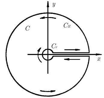
Figure 1: Integration contour $C$ ($r$ and $R$ are radii of the small and big circles respectively, where $r\ll 1$ and $R\gg 1$).

and then letting $R\to\infty\,$, $r\to 0$, we have

$$\displaystyle\ointctrclockwise\limits_{C}\frac{\,z^{x}e^{-i\pi x}\,}{\,(1+z)^{n}\,(\ln z-\pi i)\,}\,dz\,=\,\int\limits_{r}^{R}\!\ldots\,\,+\,\int\limits_{C_{R}}\!\ldots\,\,+\int\limits_{Re^{2i\pi}}^{\;re^{2i\pi}}\!\!\!\!\ldots\,\,+\,\int\limits_{C_{r}}\!\ldots\stackrel{{\scriptstyle\begin{subarray}{c}R\to\infty\\ r\to 0\end{subarray}}}{{=}}\quad$$ (168)

$$\displaystyle\;=\int\limits_{0}^{\infty}\!\left\{\frac{e^{-\pi ix}}{\ln z-\pi i}-\frac{e^{+\pi ix}}{\ln z+\pi i}\right\}\cdot\frac{z^{x}\,dz}{(1+z)^{n}}\,=\,2i\!\int\limits_{0}^{\infty}\!\frac{\,\pi\cos\pi x-\sin\pi x\ln z\,}{\,\ln^{2}z+\pi^{2}\,}\cdot\frac{z^{x}\,dz}{\,(1+z)^{n}}$$

since for $\,R\to\infty\,$

$$\left|\,\int\limits_{C_{R}}\!\frac{\,z^{x}\,e^{-i\pi x}\,}{\,(1+z)^{n}\,(\ln z-\pi i)\,}\,dz\,\right|\,=\,O\left(\!\frac{1}{\,R^{n-x-1}\ln R\,}\!\right)=o(1)\,,\qquad n\geqslant x+1\,,$$

and for $\,r\to 0\,$

$$\left|\,\int\limits_{C_{r}}\!\frac{\,z^{x}\,e^{-i\pi x}\,}{\,(1+z)^{n}\,(\ln z-\pi i)\,}\,dz\,\right|\,=\,O\left(\!\frac{\,r^{x+1}\,}{\,\ln r\,}\!\right)=o(1)\,,\qquad x\geqslant-1\,,$$

where $n\in\mathbb{N}$ and $x$ is assumed to be real. But the above contour integral may also be evaluated by means of the Cauchy residue theorem. Since the integrand has only two singularities, a branch point at $z=0$ which we excluded and a pole of the $(n+1)$th order at $z=e^{i\pi}=-1$, the Cauchy residue theorem gives us

$$\displaystyle\ointctrclockwise\limits_{C}\frac{\,z^{x}\,e^{-i\pi x}\,}{\,(1+z)^{n}\,(\ln z-\pi i)\,}\,dz\,=\,2\pi i\!\mathop{\rm res}\limits\limits_{z=-1}\!\frac{z^{x}\,e^{-i\pi x}}{\,(1+z)^{n}\,(\ln z-\pi i)\,}\,=$$ (169)

$$\displaystyle\qquad\qquad\qquad\,=\,\frac{2\pi i}{n!}\cdot\left.\frac{\partial^{n}}{\partial z^{n}}\frac{z^{x}\,e^{-i\pi x}\,(z+1)}{\,\ln z-\pi i\,}\right|_{z=-1}\!\!\!=\,2\pi i\,(-1)^{n-1}\psi_{n}(x)\,.$$

Equating (168) with (169), therefore, yields

$$\psi_{n}(x)\,=\,\frac{(-1)^{n+1}}{\pi}\!\int\limits_{0}^{\infty}\!\frac{\,\pi\cos\pi x-\sin\pi x\ln z\,}{\,(1+z)^{n}}\cdot\frac{z^{x}\,dz}{\,\ln^{2}z+\pi^{2}\,}\,,$$ (170)

where $\,n\in\mathbb{N}\,$ and $\,-1\leqslant x\leqslant n-1\,$. This formula may also be written is a variety of other forms, for example,

$$\displaystyle\psi_{n}(x) =\,\frac{(-1)^{n+1}}{\pi}\!\int\limits_{0}^{\infty}\!\frac{\,\pi\cos\pi x+\sin\pi x\ln z\,}{\,(1+z)^{n}}\cdot\frac{z^{n-x-2}\,dz}{\,\ln^{2}z+\pi^{2}\,}$$ (173)

$$\displaystyle=\,\frac{(-1)^{n+1}}{\pi}\!\int\limits_{-\infty}^{+\infty}\!\!\frac{\,\pi\cos\pi x-v\sin\pi x\,}{\,(1+e^{v})^{n}}\cdot\frac{e^{v(x+1)}}{\,v^{2}+\pi^{2}\,}\,dv$$

$$\displaystyle=\,\frac{(-1)^{n+1}}{\pi}\!\int\limits_{-\infty}^{+\infty}\!\!\frac{\,\pi\cos\pi x+v\sin\pi x\,}{\,(1+e^{v})^{n}}\cdot\frac{e^{v(n-x-1)}}{\,v^{2}+\pi^{2}\,}\,dv$$

with the same $n$ and $x$. Note that at $x=0$ we retrieve Schröder’s formulæ for $G_{n}$ [11]. ∎

References

- [1] A. Adelberg, 2-Adic congruences of Nörlund numbers and of Bernoulli numbers of the second kind, J. Number Theory, 73 (1998), 47–58.
- [2] J.-P. Allouche, M. M. France and J. Peyrière, Automatic Dirichlet series, J. Number Theory, 81 (2000), 359–373.
- [3] P. Appell, Sur la constante d’Euler, Nouv. Ann. Math (6), 1 (1925), 289–290.
- [4] P. Appell, Sur les polynomes de Fontana–Bessel, Enseign. Math., 25 (1926), 189–190.
- [5] H. Bateman and A. Erdélyi, Higher Transcendental Functions, Mc Graw–Hill Book Company, 1955.
- [6] F. W. Bessel, Untersuchung der durch das Integral ausgedrückten Function, König. Arch. Naturwiss. Math., 1 (1811), 1–40. Erratum: 1 (1811), 239–240.
- [7] Ia. V. Blagouchine, Rediscovery of Malmsten’s integrals, their evaluation by contour integration methods and some related results, Ramanujan J., 35 (2014), 21–110. Erratum–Addendum: 42 (2017), 777–781.
- [8] Ia. V. Blagouchine, A theorem for the closed–form evaluation of the first generalized Stieltjes constant at rational arguments and some related summations, J. Number Theory, 148 (2015), 537–592. Erratum: 151 (2015), 276–277.
- [9] Ia. V. Blagouchine, Expansions of generalized Euler’s constants into the series of polynomials in and into the formal enveloping series with rational coefficients only, J. Number Theory, 158 (2016), 365–396. Corrigendum: 173 (2017), 631–632.
- [10] Ia. V. Blagouchine, Two series expansions for the logarithm of the gamma function involving Stirling numbers and containing only rational coefficients for certain arguments related to , J. Math. Anal. Appl., 442 (2016), 404–434.
- [11] Ia. V. Blagouchine, A note on some recent results for the Bernoulli numbers of the second kind, J. Integer Seq., 20 (2017), 1–7. Art. 17.3.8
- [12] V. Bolbachan, New proofs of some formulas of Guillera-Ser-Sondow, arXiv:0910.4048 (2009).
- [13] G. Boole (J. F. Moulton editor), Calculus of Finite Differences (4th edn.), Chelsea Publishing Company, New-York, USA, 1957.
- [14] Yu. A. Brychkov, Power expansions of powers of trigonometric functions and series containing Bernoulli and Euler polynomials, Integral Transforms Spec. Funct., 20 (2009), 797–804.
- [15] Yu. A. Brychkov, On some properties of the generalized Bernoulli and Euler polynomials, Integral Transforms Spec. Funct., 23 (2012), 723–735.
- [16] B. Candelpergher and M.-A. Coppo, A new class of identities involving Cauchy numbers, harmonic numbers and zeta values, Ramanujan J., 27 (2012), 305–328.
- [17] B. Candelpergher and M.-A. Coppo, Le produit harmonique des suites, Enseign. Math., 59 (2013), 39–72.
- [18] L. Carlitz, Some theorems on Bernoulli numbers of higher order, Pacific J. Math., 2 (1952), 127–139.
- [19] L. Carlitz, A note on Bernoulli and Euler polynomials of the second kind, Scripta Math., 25 (1961), 323–330.
- [20] C.-P. Chen, Sharp inequalities and asymptotic series of a product related to the Euler–Mascheroni constant, J. Number Theory, 165 (2016), 314–323.
- [21] C.-P. Chen and R. B. Paris, On the asymptotic expansions of products related to the Wallis, Weierstrass and Wilf formulas, Appl. Math. Comput., 293 (2017), 30–39.
- [22] M. W. Coffey, Addison-type series representation for the Stieltjes constants, J. Number Theory, 130 (2010), 2049–2064.
- [23] M. W. Coffey, Series representations for the Stieltjes constants, Rocky Mountain J. Math., 44 (2014), 443–477.
- [24] L. Comtet, Advanced Combinatorics. The Art of Finite and Infinite Expansions (revised and enlarged edn.), D. Reidel Publishing Company, Dordrecht, Holland, 1974.
- [25] D. F. Connon, Some series and integrals involving the Riemann zeta function, binomial coefficients and the harmonic numbers. Volume II(a), arXiv:0710.4023 (2007).
- [26] D. F. Connon, Some series and integrals involving the Riemann zeta function, binomial coefficients and the harmonic numbers. Volume II(b), arXiv:0710.4024 (2007).
- [27] D. F. Connon, Some possible approaches to the Riemann hypothesis via the Li/Keiper constants, arXiv:1002.3484 (2010).
- [28] H. T. Davis, The approximation of logarithmic numbers, Amer. Math. Monthly, 64 (1957), part II, 11–18.
- [29] L. Fekih-Ahmed, On the zeros of the Riemann zeta function, arXiv:1004.4143 (2010).
- [30] S. R. Finch, Mathematical Constants, Cambridge University Press, USA, 2003.
- [31] P. Flajolet and R. Sedgewick, Mellin transforms and asymptotics: Finite differences and Rice’s integrals, Theoret. Comput. Sci., 144 (1995), 101–124.
- [32] F. Franklin, On an expression for Euler’s constant, John Hopkins Univ. Circulars, II(25) (1883/1888), 143.
- [33] H. H. Goldstine, A History of Numerical Analysis from the 16th through the 19th Century, Springer–Verlag, New–York, Heidelberg, Berlin, 1977.
- [34] H. W. Gould, Stirling number representation problems, Proc. Amer. Math. Soc., 11 (1960), 447–451.
- [35] H. W. Gould, Note on recurrence relations for Stirling numbers, Publ. Inst. Math. (N.S.), 6 (1966), 115–119.
- [36] R. W. Hamming, Numerical Methods for Scientists and Engineers, McGraw–Hill Book Company, 1962.
- [37] H. Hasse, Ein Summierungsverfahren für die Riemannsche -Reihe, Math. Z., 32 (1930), 458–464.
- [38] Ch. Hermite, Extrait de quelques lettres de M. Ch. Hermite à M. S. Pincherle, Ann. Mat. Pura Appl. (3), 5 (1901), 57–72.
- [39] F. T. Howard, Nörlund number , in “Applications of Fibonacci Numbers, 5, 355–366”, Kluwer Academic, Dordrecht, 1993.
- [40] H. Jeffreys and B. S. Jeffreys, Methods of Mathematical Physics (2nd edn.), University Press, Cambridge, Great Britain, 1950.
- [41] Ch. Jordan, Sur des polynomes analogues aux polynomes de Bernoulli, et sur des formules de sommation analogues à celle de Maclaurin–Euler, Acta Sci. Math. (Szeged), 4 (1928–1929), 130–150.
- [42] Ch. Jordan, The Calculus of Finite Differences (3rd edn.), Chelsea Publishing Company, New-York, USA, 1965.
- [43] L. V. Kantorovich and V. I. Krylov, Approximate Methods of Higher Analysis (3rd edn., in Russian), Gosudarstvennoe izdatel’stvo fiziko–matematicheskoi literatury, Moscow, USSR, 1950.
- [44] J. C. Kluyver, Euler’s constant and natural numbers, Proc. K. Ned. Akad. Wet., 27 (1924), 142–144.
- [45] V. Kowalenko, Properties and applications of the reciprocal logarithm numbers, Acta Appl. Math., 109 (2010), 413–437.
- [46] V. I. Krylov, Approximate Calculation of Integrals, The Macmillan Company, New-York, USA, 1962.
- [47] D. H. Lehmer, The sum of like powers of the zeros of the Riemann zeta function, Math. Comp., 50 (1988), 265–273.
- [48] M. Lerch, Expressions nouvelles de la constante d’Euler, Věstník Královské české společnosti náuk. Tř. mathematicko-přírodovědecká, 42 (1897), 1–5.
- [49] Y. L. Luke, The Special Functions and their Approximations, Academic Press, NewYork, 1969.
- [50] P. V. Melentiev, Approximate Calculations (in Russian), Gosudarstvennoe izdatel’stvo fiziko–matematicheskoi literatury, Moscow, USSR, 1962.
- [51] D. Merlini, R. Sprugnoli and M. Cecilia Verri, The Cauchy numbers, Discrete Math., 306 (2006), 1906–1920.
- [52] W. E. Milne, Numerical Calculus: Approximations, Interpolation, Finite Differences, Numerical Integration and Curve Fitting, Princeton University Press, Princeton, 1949.
- [53] M. L. Milne-Thomson, The Calculus of Finite Differences, MacMillan and Co., Limited, London, 1933.
- [54] A. D. Morgan, The Differential and Integral Calculus, Baldwin & Cradock, London, 1842.
- [55] G. Nemes, Generalization of Binet’s gamma function formulas, Integral Transforms Spec. Funct., 24 (2013), 597–606
- [56] N. E. Nörlund, Mémoire sur les polynomes de Bernoulli, Acta Math., 43 (1922), 121–196.
- [57] N. E. Nörlund, Vorlesungen über Differenzenrechnung, Springer, Berlin, 1924.
- [58] N. E. Nörlund, Sur les valeurs asymptotiques des nombres et des polynômes de Bernoulli, Rend. Circ. Mat. Palermo, 10 (1961), 27–44.
- [59] G. M. Phillips, Interpolation and Approximation by Polynomials, Springer, New–York, 2003.
- [60] F. Qi, An integral representation, complete monotonicity, and inequalities of Cauchy numbers of the second kind, J. Number Theory, 144 (2014), 244–255.
- [61] S. Roman, The Umbral Calculus, Academic Press, NewYork, 1984.
- [62] M. O. Rubinstein, Identities for the Riemann zeta function, Ramanujan J., 27 (2012), 29–42.
- [63] H. E. Salzer, Coefficients for numerical integration with central differences, Phil. Mag., 35 (1944), 262–264.
- [64] J. Ser, Questions 5561–5564, Intermédiaire Math. (2), 4 (1925), 126–128.
- [65] J. Ser, Sur une expression de la fonction de Riemann, C. R. Acad. Sci. Paris (2), 182 (1926), 1075–1077.
- [66] R. Sitaramachandrarao, Maclaurin coefficients of the Riemann zeta function, Abstr. Papers Presented Amer. Math. Soc., 7 (1986), 280.
- [67] D. V. Slavić, Classification with generalizations of quadrature formulas, Univ. Beograd Publ. Elektrotehn. Fak. (Mat. Fiz.), 735–762 (1982), 102–121.
- [68] J. Soldner, Théorie et Tables d’une Nouvelle Fonction Transcendante, Lindauer, Minuc, 1809.
- [69] J. Sondow, Analytic continuation of Riemann’s zeta function and values at negative integers via Euler’s transformation of series, Proc. Amer. Math. Soc., 120 (1994), 421–424.
- [70] J. Sondow and S. A. Zlobin, Integrals over polytopes, multiple zeta values and polylogarithms, and Euler’s constant, Math. Notes, 84 (2008), 568–583.
- [71] É. Picard (editor), Œuvres de Charles Hermite, Gauthier-Villars, Paris, 1905–1917.
- [72] S. C. Van Veen, Asymptotic expansion of the generalized Bernoulli numbers for large values of ( integer), Indag. Math., 13 (1951), 335–341.
- [73] G. Vacca, Sulla costante di Eulero, , Atti Accad. Naz. Lincei, Classe di scienze fisiche, matematiche e naturali (6), 1 (1925), 206–210.
- [74] N. N. Vorobiev, Theory of Series (4th edn., in Russian), Nauka, Moscow, USSR, 1979.
-
[75]
E. W. Weisstein, Euler-mascheroni constant, From MathWorld–A Wolfram
Web Resource, published electronically at
http://mathworld.wolfram.com/Euler-MascheroniConstant.html - [76] E. Whittaker and G. Robinson, The Calculus of Observations. A Treatise on Numerical Mathematics, Blackie and Son Limited, London, 1924.
- [77] C. Xu, Y. Yan and Z. Shi, Euler sums and integrals of polylogarithm functions, J. Number Theory, 165 (2016), 84–108.
- [78] P. T. Young, Congruences for Bernoulli, Euler and Stirling numbers, J. Number Theory, 78 (1999), 204–227.
- [79] P. T. Young, Rational series for multiple zeta and log gamma functions, J. Number Theory, 133 (2013), 3995–4009.
- [80] F.-Z. Zhao, Sums of products of Cauchy numbers, Discrete Math., 309 (2009), 3830–3842.