Solving the Dynamic Correlation Problem of the Susceptible-Infected-Susceptible Model on Networks

Abstract

The susceptible-infected-susceptible (SIS) model is a canonical model for emerging disease outbreaks. Such outbreaks are naturally modeled as taking place on networks. A theoretical challenge in network epidemiology is the dynamic correlations coming from that if one node is infected, then its neighbors are likely to be infected. By combining two theoretical approaches–the heterogeneous mean-field theory and the effective degree method–we are able to include these correlations in an analytical solution of the SIS model. We derive accurate expressions for the average prevalence (fraction of infected) and epidemic threshold. We also discuss how to generalize the approach to a larger class of stochastic population models.

The susceptible-infected-susceptible (SIS) model is a fundamental model of outbreaks of diseases (like influenza, chlamydia, gonhorrea, etc.) that does not give immunity upon recovery. Diseases spread over networks of people and the structure of these networks affect spreading Keeling and Eames (2005); thus, it makes sense to put the SIS model on networks. The SIS model divides the population into two classes–susceptible (S) and infected (I). Links between S and I transmit the disease (i.e. make the susceptible infected) with a rate $r$. Infected individuals become susceptible again with a rate $g$. One can reduce these two parameters to one–$\lambda=r/g$–the rate of new infections per SI link per recovery, or the effective infection rate. In the thermodynamic limit $N\rightarrow\infty$, there can be a threshold, or phase-transition phenomenon when tuning $\lambda$ Marro and Dickman (1999). For $\lambda$ less than a critical $\lambda_{c}$ the disease dies out spontaneously. If $\lambda>\lambda_{c}$ the disease will live forever–i.e. it has reached an endemic state where the prevalence $\rho$ (fraction of infected nodes) is nonzero. Also, for finite networks, there is effectively an endemic state as the expected extinction time, even for small networks, grows extremely fast beyond $\lambda_{c}$ Holme (2015). The two main directions in the literature are to study extinction times in finite, homogeneous networks Nåsell (2001) or how the threshold depends on the network structure Pastor-Satorras and Vespignani (2001); Barrat et al. (2008). This work belongs to the latter class.

For the SIS model in a well-mixed population, the threshold happens at $\lambda_{c}=1$ Hethcote (2000). For the SIS model in homogeneous networks, such as the Erdős-Rényi random networks and random regular graphs, a simple approximative (mean-field) analysis gives the threshold $\lambda_{c}=1/\langle k\rangle$ Pastor-Satorras and Vespignani (2001). For the SIS model in scale-free networks Albert and Barabási (2002)–where the degree distribution (the probability that a random node is connected to $k$ other nodes) follows $P(k)\sim k^{-\gamma}$–heterogeneous mean-field theory predicts that the epidemic threshold of the SIS model is equal to that of the susceptible-infected-recovered (SIR) model $\lambda_{c}^{\mathrm{HMF,SIS}}=\lambda_{c}^{\mathrm{HMF,SIR}}=\langle k\rangle/\langle k^{2}\rangle$ Pastor-Satorras and Vespignani (2001); Dorogovtsev et al. (2008); Barrat et al. (2008); Ferreira et al. (2012). In other words, the threshold seems to be zero for $\gamma\leq 3$, and finite for $\gamma>3$ Pastor-Satorras et al. (2015). The heterogeneous mean-field theory is a degree-based mean-field theory, which sorts the nodes into different classes in terms of the magnitude of their degrees, but all the other aspects are considered totally random (for instance, who connects whom). In other words, the heterogeneous mean-field theory neglects correlation, both from the disease dynamics (a node is more likely infected if its neighbors are infected) and the network structure. Effectively, the heterogeneous mean-field theory applies to a situation where the network is constantly rewired (or annealed) at a time scale faster than the disease dynamics. (See the Supplemental Material sm for more details on the SIS and SIR models on annealed networks)

Moving beyond the heterogeneous mean-field assumption that the network is rapidly changing, we have to deal with dynamic correlations. In the heterogeneous mean-field, the probability to be infected is $\rho$ for two nodes of the same degree, but because of dynamic correlations a node is more likely to be infected if many of its neighbors are infected. This fact–the probability of having an already infected neighbor is larger than in the mean-field approximation–will reduce the effective infection rate, and thus the speed and extent of the disease propagation. One possible remedy is to consider an individual-based mean-field approximation by taking into account the full network structure correlation (still ignoring the dynamic correlations). This is also called the quenched mean-field theory Van Mieghem et al. (2009); Granell et al. (2013). The quenched mean-field theory gives the epidemic threshold $\lambda_{c}^{\mathrm{QMF,SIS}}=1/\Lambda_{1}$ Van Mieghem et al. (2009), where $\Lambda_{1}$ is the largest eigenvalue of the adjacency matrix of the underlying network. According to Ref. Chung et al. (2003), for scale-free networks,

$$1/\Lambda_{1}\sim\left\{\begin{array}[]{cl}1/\sqrt{k_{\mathrm{max}}},&\gamma>5/2,\\ \langle k\rangle/\langle k^{2}\rangle,&2<\gamma<5/2,\\ \end{array}\right.$$ (1)

where $k_{\mathrm{max}}$ is the maximum degree in the network. Both the heterogeneous mean-field and quenched mean-field methods imply that the epidemic threshold in scale-free networks vanishes in the thermodynamic limit, but remains finite for networks of finite sizes. Some numerical studies suggest that the quenched mean-field is qualitatively correct in scale-free networks Castellano and Pastor-Satorras (2010); Boguñá et al. (2013), but others point at deviations from the threshold value Ferreira et al. (2012).

There are studies that do take dynamic correlations into account. This, so called, effective degree approach Lindquist et al. (2011); Cai et al. (2014) is a higher order degree-based mean-field theory, explicitly considering the dynamic correlation between directly connected neighbors. It does indeed provides a much more accurate prediction of the epidemic threshold for the SIR model in uncorrelated networks, $\lambda_{c}^{\mathrm{ED,SIR}}=\frac{\langle k\rangle}{\langle k^{2}\rangle-2\langle k\rangle}$ Lindquist et al. (2011). This works by mapping the SIR process to a bond-percolation problem Pastor-Satorras et al. (2015); Grassberger (1983), but has not yet been applied to the SIS model. Boguñá et al. Boguñá et al. (2013) take dynamic correlation between distant neighbors into account within the framework of quenched mean-field theory. They replaced the original SIS dynamics by a modified process valid over coarse-grained times and argued that dynamic correlation changes the dynamics near the threshold. Based on a spectral approach, which takes into account the other eigenvectors of the adjacency matrix than $\Lambda_{1}$, Goltsev et al. Goltsev et al. (2012) showed that in scale-free networks with $\gamma>5/2$, the principal eigenvector is localized when the effective infection rate is slightly above $\lambda_{c}^{\mathrm{QMF,SIS}}$. Since in quenched mean field theory the density of infected vertices is proportional to the principal eigenvector, their work predicts a transition to a localized phase, where the activity is concentrated to the hubs and their immediate neighbors. Ferreira et al. Ferreira et al. (2016) studied the relationship between the hub lifespan and the hub infection time to discern the nature of the threshold in general epidemic models on scale-free networks. Reference Ruhi et al. presents yet further refinements of the quenched mean-field theory. Finally, in this literature review, we also want to mention many other approaches to understand SIS or SIR processes on networks, such as: the fluctuation theory Lee et al. (2013), the pair-approximation method Eames and Keeling (2002); Kiss et al. (2015), probability generating function techniques Newman (2002); Volz and Meyers (2007), $R_{0}$-based modification Aparicio and Pascual (2007), percolation theory Newman (2002); Parshani et al. (2010), and branching process Leventhal et al. (2015), etc. However, all these methods depend on large sets of coupled ordinary differential equations, and are unable to provide explicit analytical solutions for the prevalence, in particular, for large-scale networks Pastor-Satorras et al. (2015).

Our current understanding of the SIS dynamics on heterogeneous networks is far from complete. In this Letter, we combine the idea of the heterogeneous mean-field theory with the effective degree approach to study the effect of dynamic correlation present in static networks on the SIS epidemic dynamics. The underlying static networks can have arbitrary degree distributions. However, we focus on networks without degree-degree correlations or other (e.g. mesoscopic) structures. Our method gives a closed-form analytical solution for the epidemic prevalence $\rho$, from which we immediately can obtain the epidemic threshold by solving the equation $\rho=0$. We further show that our method matches numerical simulations better than the above-mentioned theory.

To begin, we define $p_{k}$ and $q_{k}$, respectively, as the probabilities of reaching an arbitrary infected individual by following a randomly chosen edge from susceptible and infected individuals of degree $k$. In the framework of heterogeneous mean-field theory where the underlying network is treated as annealed, the value of $q_{k}$ is always equal to that of $p_{k}$ Boguñá et al. (2013). For the earlier mentioned reasons, the dynamic correlations mean that

$$q_{k}>p_{k}.$$ (2)

In the spirit of the heterogeneous mean-field Pastor-Satorras and Vespignani (2001), we can write down the master equation for those infected individuals of degree class $k$,

$$\frac{dI_{k}(t)}{dt}=-I_{k}(t)g+rkS_{k}(t)p_{k}(t),$$ (3)

where $S_{k}(t)$ and $I_{k}(t)$ are the number of susceptible and infected individuals with degree $k$ at time $t$, respectively. The first term represents the spontaneous recovery and the second one the newly emerged infection in class $k$ due to the interaction with other classes. In the steady state, we have

$$p_{k}=\frac{g}{kr}\frac{I_{k}}{S_{k}}.$$ (4)

In annealed networks, one assumes $p_{k}=q_{k}=\frac{1}{\langle k\rangle N}\sum_{k}kI_{k}$, where $N$ is the total population size, to continue the theoretical derivation. As mentioned above, this hypothesis is not applicable for the SIS model in static networks. In what follows, we circumvent this problem following the effective degree approach. This means that we divide the network into classes representing both the state of an individual and its neighbors Gleeson (2011, 2013). Let $S_{k,j}(t)$ $[I_{k,j}(t)]$ be the density of $k$ degree nodes that are susceptible (infected) at time $t$, connected to $j$ infected neighbors. Then $S_{k,j}(t)$ and $I_{k,j}(t)$ can be written as

$$S_{k,j}(t) = S_{k}(t)\left[1-p_{k}(t)\right]^{k-j}\left[p_{k}(t)\right]^{j}{k\choose j},$$ (5a)

$$I_{k,j}(t) = I_{k}(t)\left[1-q_{k}(t)\right]^{k-j}\left[q_{k}(t)\right]^{j}{k\choose j},$$ (5b)

where $S_{k}(t)=\sum_{j}S_{k,j}(t)$ and $I_{k}(t)=\sum_{j}I_{k,j}(t)$. Summing over all possible events, we obtain the total recovery rate $a(t)=\sum_{k}\sum_{j}I_{k,j}(t)g$ and the population-level transmission rate $b(t)=\sum_{k}\sum_{j}S_{k,j}(t)jr$. When the system is in its steady state, the total recovery rate must be equal to the total transmission rate, satisfying the detailed balance conditions $a=b$ and $\langle\Delta a\rangle=\langle\Delta b\rangle$, where $\Delta a$ and $\Delta b$ are the changing rate of $a$ and $b$ in the time interval $dt$ (where only one event occurs). All possible values of these two quantities in a static network are summarized in Table 1. With these preliminary results, we have

$$\sum_{k}\sum_{j}S_{k,j}j^{2}r=\sum_{k}\sum_{j}I_{k,j}jg.$$ (6)

Note that the formula of Eq. (6) is exact for the steady state in any static networks. Nevertheless, we want to point out that they are not applicable to irreversible processes such as the SIR model.

Table 1: All possible situations in a time interval $dt$ of the SIS process in a static network.

Situation	Probability	$\Delta a$	$\Delta b$
$S_{k,j}\rightarrow I_{k,j}$	$\frac{S_{k,j}(t)jr}{a+b}$	$+g$	$-jr+r(k-j)$
$I_{k,j}\rightarrow S_{k,j}$	$\frac{I_{k,j}(t)g}{a+b}$	$-g$	$+jr-r(k-j)$

Using the condition that the total number of infectious neighbors of all susceptible individuals equals the total number of susceptible neighbors of all infectious individuals Keeling (1999), we get the relationship $\sum_{k}\sum_{j}I_{k,j}jg=g\sum_{k}I_{k}[k-g/r]$. Combining this with Eqs. (4) and (6), gives

$$g\sum_{k}I_{k}\left[(k-1)p_{k}+1-k+\frac{g}{r}\right]=0.$$ (7)

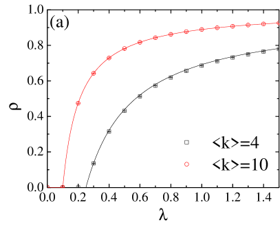
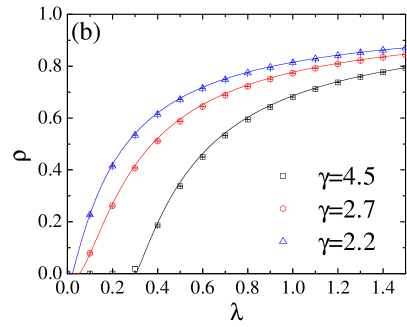
Figure 1: The epidemic prevalence $\rho$ is plotted as a function of the effective infection rate $\lambda$ in static networks. (a) Erdős-Rényi random networks with average degree $4$ and $10$, (b) scale-free network with minimum degree $3$ and $\gamma=4.5$, $2.7$, and $2.2$. Lines are theoretical estimations of Eqs. (9) and (11), while the points are simulation results. We use networks with $N=10^{5}$ nodes and $100$ randomly chosen seeds for the infection. Each data point is an average over at least $100$ independent epidemic outbreaks, performed on at least $10$ different network realizations.

Notice that only infected individuals can determine the birth and death of susceptible individuals, but not vice versa. Any new infection or recovery event will mainly change the difference among various $q_{k}$ (since the probability of finding connected infected pair with certain degrees will increase or decrease definitely due to the event). But it does not provide any valuable hints about how various $p_{k}$ will differ from each other (albeit their values would change owing to the newly emerged or disappeared infected individual) for degree-uncorrelated random networks. In light of the maximum entropy principle Jaynes (1957), we assume all $p_{k}$ change with the same magnitude such that they always satisfy the following approximative relations

$$p_{1}\simeq p_{2}\simeq\cdots\simeq p_{k_{\mathrm{max}}}=p.$$ (8)

That is to say, our method is mainly concerned about the dynamic correlations present in connected infected pairs, but neglects higher-order dynamic correlations in susceptible-susceptible or susceptible-infected pairs. We have verified that Eqs. (2) and (8) capture the most important parts of the dynamic correlations, neglecting only minor ones sm . Substituting Eq. (8) into Eqs. (4) and (7), we obtain the iterative equation

$$I_{k}=\frac{\lambda kp}{1+\lambda kp}N_{k},$$ (9)

where $p$ itself is a function of $I_{k}$ as

$$p=1-\frac{I}{\lambda\sum_{k}I_{k}(k-1)}.$$ (10)

Combining with Eqs. (9) and (10), we can find the solution of $p$, which is now a function of $\lambda$, satisfying the self-consistency equation

$$(1-p)\lambda\sum_{k}(k-1)\frac{\lambda kp}{1+\lambda kp}NP(k)-\sum_{k}\frac{\lambda kp}{1+\lambda kp}NP(k)=0.$$ (11)

Now we are able to calculate the epidemic prevalence $\rho$ in the steady state as follows: (i) Calculate $p$ from Eq. (11); (ii) Substitute the value of $p$ into Eq. (9) to solve $I_{k}$; (iii) Obtain the epidemic prevalence $\rho=\frac{1}{N}\sum_{k}I_{k}$. The results are summarized in Fig. 1, from which we can see that the estimations obtained by our approach match those from stochastic simulations quite well sm .

A nonzero stationary epidemic prevalence is obtained when the $p$ has a nontrivial solution in the interval $0<p\leq 1$. We denote the left-hand side of Eq. (11) by $f(p)$. It is easy to see that $p=0$ is a trivial solution of Eq. (11). Furthermore, note that $f(p)$ is always negative for $p=1$. Hence, the condition that $p$ has a meaningful solution in the interval $(0,1]$ reads as

$$\frac{d}{dp}f(p)\bigg{|}_{p=0}\geq 0.$$ (12)

The value of $\lambda$ satisfying the equality of the above inequality determines the epidemic threshold $\lambda_{c}$, whose value is given, for uncorrelated random networks, by

$$\lambda_{c}=\frac{\langle k\rangle}{\langle k^{2}\rangle-\langle k\rangle}.$$ (13)

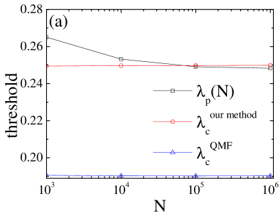
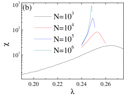
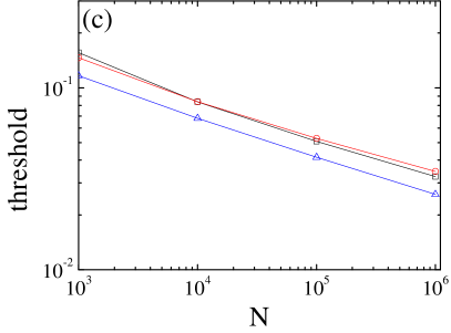
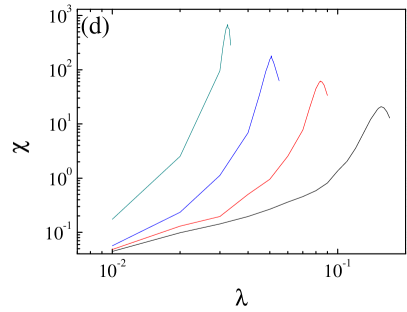
Figure 2: (a) and (c) Epidemic threshold $\lambda_{c}$, obtained by our method, the quenched mean-field method, and the quasistationary state method Ferreira et al. (2012), versus network size $N$. (b) and (d) Susceptibility $\chi$ as a function of the effective infection rate $\lambda$ for varying network size $N$, where the peak values determine the $\lambda_{p}(N)$ in (a) and (c). Panels (a) and (b) are for Erdős-Rényi random networks with average degree $\langle k\rangle=4$; (c) and (d) are for scale-free networks with minimum degree $3$ and $\gamma=2.7$. The results are obtained for the epidemic dynamics over at least ten different network realizations with initial infected seed number $I_{0}=1$.

The epidemic threshold of the SIS model obtained by our method is larger than the one predicted by the heterogeneous mean-field theory Pastor-Satorras and Vespignani (2001); Dorogovtsev et al. (2008); Barrat et al. (2008); Ferreira et al. (2012), and is smaller than the threshold of the SIR model by the effective degree approach Lindquist et al. (2011); Pastor-Satorras et al. (2015). Equation (13) implies that the epidemic threshold of the SIS epidemic process is zero for scale-free networks with $\gamma<3$, but finite if $\gamma>3$. This is consistent with the conclusions of previous work using other methods Goltsev et al. (2012); Lee et al. (2013). In Fig. 2, we plot the epidemic thresholds against network size and show that, in Erdős-Rényi and scale-free random networks, the accuracy of the epidemic threshold of our method is better than that of the quenched mean-field theory, and matches the results from the quasistationary numerical simulation well Ferreira et al. (2012).

To provide further evidence on the efficiency of our proposed approach, we consider the SIS model in a random regular graph whose degree distribution is a Kronecker’s delta function $P(k)=\delta_{kk_{0}}$; i.e., each node in a random regular graph has a degree of $k_{0}$ and all the other aspects are totally random. From Eqs. (4) and (7), we can acquire the epidemic prevalence

$$\rho=1-\frac{1}{1+k_{0}(\lambda-\frac{1}{k_{0}-1})},$$ (14)

where $\lambda=r/g$ is again the effective infection rate. From Fig. 3(a), we can see that the results from the analytical solution of Eq. (14) are in excellent agreement with those obtained from stochastic simulations in a static random regular graph.

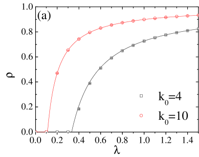
Figure 3: (a) The epidemic prevalence $\rho$ is plotted as a function of the effective infection rate $\lambda$ in static random regular graphs with degree $k_{0}=4$ and $10$. Lines are the theoretical predictions of Eq. (14), while the scatters are Monte Carlo simulation results. Other parameters are the same as those in Fig. 1. (b) Susceptibility $\chi$ as a function of the effective infection rate $\lambda$ for random regular graphs with different network sizes, where $k_{0}$ is fixed to 5.

For the epidemic threshold of the SIS model in static random regular graphs, the prediction of the quenched mean-field theory can easily be simplified to $\lambda_{c}^{\mathrm{QMF}}=1/k_{0}$ by applying the Perron-Frobenius theorem Ferreira et al. (2012). By means of the pair-approximation method, a more accurate estimation of epidemic threshold, $\lambda_{c}^{\text{pair}}=1/(k_{0}-1)$, is reported Eames and Keeling (2002). Very recently, by combining the branching process with the probability generating function, Leventhal et al. obtained the same threshold $1/(k_{0}-1)$ Leventhal et al. (2015). For our case, we just need to set $\rho=0$ in Eq. (14), and then the epidemic threshold can be obtained directly as

$$\lambda_{c}=\frac{1}{k_{0}-1},$$ (15)

which is consistent with the findings in Refs. Eames and Keeling (2002); Leventhal et al. (2015). In Fig. 3(b), we plot the susceptibility against the effective infection rate $\lambda$ in static random regular graph with degree $k_{0}=5$, and show that the susceptibility peak is closer to the theoretical prediction of Eq. (15) than to the quenched mean-field result Ferreira et al. (2012), once again validating our method.

Thus, the combination of the heterogeneous mean-field theory and the effective degree method enables us to, on one hand, include dynamic correlation and network-structural correlation (to a necessary extent) to obtain more accurate predictions (than in previous works) of both the epidemic prevalence and threshold, and on the other hand obtain explicit expressions for these two quantities.

As a final analysis, we extended our method to the case of contact process Castellano and Pastor-Satorras (2006)–where infected individuals meet random neighbors for possible contagion events–on random regular graph networks with degree $k_{0}$. According to the heterogeneous mean-field theory, we have $p=\frac{g}{r}\frac{I_{k_{0}}}{S_{k_{0}}}$. The total recovery and transmission rates of the whole population are $a=\sum_{j}I_{k_{0},j}g$ and $b=\sum_{j}S_{k_{0},j}jr\frac{1}{k_{0}}$, respectively. Equation (6) will now be replaced by $\frac{r}{k_{0}}\sum_{j}S_{k_{0},j}j^{2}=g\sum_{j}I_{k_{0},j}j$. Then, we can straightforwardly derive the prevalence as

$$\rho=1-\frac{1}{1+\lambda-\frac{k_{0}}{k_{0}-1}}.$$ (16)

Accordingly, the epidemic threshold of the contact process on random regular graphs is given by

$$\lambda_{c}=\frac{k_{0}}{k_{0}-1}.$$ (17)

This epidemic threshold is also consistent with previously reported results Ferreira et al. (2011); Muñoz et al. (2010); see more details in sm .

In summary, we have studied the impact of dynamic correlations, naturally arising in spreading processes on static networks, on the SIS epidemics. In particular, we take into account the dynamic correlation from infected pairs, but ignore those from other node pairs and higher-order network structure, to derive the master equations governing the state evolution of the system. By combining the idea of the heterogeneous mean-field theory with the effective degree approach, we are able to obtain the epidemic prevalence of the SIS process in uncorrelated static networks with arbitrary degree distributions with a higher precision than other approaches. It is worth noting that the epidemic threshold can be calculated as a corollary of the epidemic prevalence. Specifically, for SIS in scale-free networks, the quenched mean-field theory predicts that the epidemic threshold is zero in the thermodynamic limit. By contrast, our theoretical results show that it remains finite for scale-free networks with $\gamma>3$, even in the thermodynamic limit.

Our work can be generalized to more general stochastic-logistic models of density dependent population dynamics Ovaskainen and Meerson (2010). In such cases, both the infection and recovery rates usually depend on the ratio $I/N$ in these models (and $I$ is often interpreted as the population size, while $N$ is the carrying capacity). Our dynamic correlation approach could be fairly straightforwardly extended to the general stochastic logistic model where Eq. (3) is the first equation to be modified (to account for the population-dependent death rate).

Note added. When the main part of this paper is ready for publication in PRL, we received several useful comments from Dr. Silvio Ferreira. Specifically, Ferreira and coworkers have also considered the dynamic correlation problem of the SIS model (and also the contact process) in quenched static networks by introducing three-vertex approximation Ferreira and Ferreira (2013) and pair quenched mean-field theory Mata, Ang lica S. and Ferreira, Silvio C. (2013). Particularly, by using a heterogeneous pair-approximation Mata et al. (2014), they also found that the epidemic threshold of the SIS process on static network reads as Eq. (13). We thank Dr. Silvio Ferreira for bringing these interesting works to our attention. We would also like to point out that our theoretical analysis of the SIS model (which is mainly based on the detailed balance equilibrium condition and the maximal entropy principle) is devoted to explicitly derive analytical expression for the prevalence in the stationary state, and the epidemic threshold can then be calculated as a corollary of the prevalence. Based on some heuristic arguments, it was shown that small-world random networks with a degree distribution decaying slower than an exponential have a vanishing epidemic threshold in the thermodynamic limit Boguñá et al. (2013). This point was also set in a more general context in Ferreira et al. (2016). In addition, for the contact process in random graphs with power law degree distributions, a rigorous proof for the vanishing epidemic threshold was provided by Chatterjee and Durret in Ref. Chatterjee and Durrett (2009). From the result presented in Refs. Ferreira et al. (2012); Mata, Ang lica S. and Ferreira, Silvio C. (2013); Mata and Ferreira (2015); Cota et al. (2016), we observed that there are usually two peaks for the susceptibility against infection rate, which is obtained by quasistationary simulation of the SIS model in scale-free networks with $\gamma>3$. For this peculiar characteristic of the SIS process on scale-free networks, we argue that there might exist two epidemic thresholds (hinted by the two peaks): One (the left peak) corresponds to the case that the amount of infected nodes becoming from zero to nonzero in the long time limit (which also can be regarded as the localized state Goltsev et al. (2012), i.e., the epidemic can only persist between connected hub nodes); The other (the right peak) corresponds to the case that the fraction of infected becomes from zero to nonzero in the thermodynamic limit (i.e., the fraction of infected could be kept as a non-zero stationary level). We think that, in localized state, the infected nodes are restricted to the hubs, and the fraction of infected becomes vanishing small in the thermodynamic limit. Thus, Our current understanding for the SIS model on (quenched) static networks from quasistationary simulations with increasing $\lambda$ could be summarized as follows: (1) For sufficiently small $\lambda$, there are null infected, i.e., the number of infected nodes goes to zero in the long time limit; (2) With the increase of $\lambda$, the epidemic can maintain active between hubs, and the nodes with small degrees are relatively difficult to be infected; (3) With the even increase of $\lambda$, the collective activation process emerges, i.e., the fraction of infected will maintain a nonzero-level in the thermodynamic limit. We thought that the studies implemented in Refs. Boguñá et al. (2013); Ferreira et al. (2016); Chatterjee and Durrett (2009) focus more on the process $(1)\rightarrow(2)$, while our proposed method and HMF theory focus more on the process $(2)\rightarrow(3)$. In this sense, we think that our current theoretical analysis gives reasonable prediction for the epidemic threshold (on scale free networks with $\gamma>3$), which suggests the system will transit from (2) to (3) with a finite threshold indicated by Eq. (13). Once again, we would like to thank Dr. Ferreira for bringing these important literature to our attention and his instructive comments on the epidemic threshold of SIS model on heterogeneous networks.

See ./sm/sm-01.pdf See ./sm/sm-02.pdf See ./sm/sm-03.pdf See ./sm/sm-04.pdf See ./sm/sm-05.pdf See ./sm/sm-06.pdf See ./sm/sm-07.pdf See ./sm/sm-08.pdf See ./sm/sm-09.pdf See ./sm/sm-10.pdf