Formal refinement of extended state machines
Abstract
In a traditional formal development process, e.g. using the B method, the informal user requirements are (manually) translated into a global abstract formal specification. This translation is especially difficult to achieve. The Event-B method was developed to incrementally and formally construct such a specification using stepwise refinement. Each increment takes into account new properties and system aspects. In this paper, we propose to couple a graphical notation called Algebraic State-Transition Diagrams (astd) with an Event-B specification in order to provide a better understanding of the software behaviour. The dynamic behaviour is captured by the astd, which is based on automata and process algebra operators, while the data model is described by means of an Event-B specification. We propose a methodology to incrementally refine such specification couplings, taking into account new refinement relations and consistency conditions between the control specification and the data specification. We compare the specifications obtained using each approach for readability and proof complexity. The advantages and drawbacks of the traditional approach and of our methodology are discussed. The whole process is illustrated by a railway CBTC-like case study. Our approach is supported by tools for translating astd’s into B and Event-B into B.
Keywords: Refinement, astd, Classical B, Event-B, Process Algebra, Railway System
1 Introduction
Specifying a system with formal languages is not straightforward. Our main objective is to specify a whole safety-critical system by using only formal notations and techniques. For validating the whole modelling process, we focus on a railway case study.
The new methodology introduced in this paper is based on the coupling of formal notations and on the joint refinement of both parts of the model. The choice of a specification language is often difficult and depends on the characteristics of the system to be specified. Most often, several languages are good candidates, but none of them, if taken alone, really fits well, because some aspects of the requirements would not be explicitely taken into account. For instance, when we first consider a state-based formal language like B [3], safety properties are well captured, but dynamic properties like ordering or liveness properties are not straightforward to express and verify. Likewise, an event-based formal language like CSP [17] or LOTOS [6] is more convenient for representing dynamic properties, but data models are difficult to capture in these languages. In addition to this issue, some syntactical, semantical or technical specificities of a language may constrain a specifier in describing the system. For instance, if there is no modularity or refinement, some systems are difficult to model ex nihilo.
In those circumstances, the coupling of specification languages may bring a solution. The aim is to take advantage of the benefits of each notation. However, coupling two distinct formal languages is not an easy task. Syntactically, such an approach must provide a way for reusing the existing notations, especially language operators, in order to be easily understood by people used to specify with one or the other language. Semantically, the different parts of the model must be consistent, so the approach must provide techniques in order to ensure that. Technically, existing tools supporting one or the other language should be reused, as much as possible.
One of the main issues with such couplings comes from the development of the whole system. Concepts like refinement are then required. Instead of writing a complete specification for the whole system in one single step, the different features are specified step by step. In the context of coupling of specification languages, these techniques are even more tricky. For instance, refinement of one part of the model must not introduce inconsistencies with respect to the other part. Sometimes, refinement is considered only in one part of the model in order to prevent that. An embedding of one language into the other one then ensures the consistency of the whole model. Recent work [22, 19, 26, 5] try either to define a formal language with a unifying semantics, or to define proof obligations generation rules for showing in which conditions one piece of specification can be refined without introducing inconsistencies.
In our approach, a formal graphical notation, called astd [13], is combined with B-like state-based formal specifications for describing the system. The dynamic behaviour is captured with an astd, which is based on automata and process algebra operators, while the data model is described by means of B-like specifications. These formal languages will be detailed in Section 2. As a main contribution, we explore complementarity and consistency between astd and B-like refinements. Section 3 introduces the main principles of our methodology. The case study is detailed in Sect. 4. Section 5 concludes the paper with some perspectives.
2 Background
2.1 B and Event-B
B is a formal method [3] supporting the main stages of the software development life cycle. Specifications are composed of abstract machines, which encapsulate state variables, an invariant constraining the state variables, an initialisation of all the state variables, and operations on the state variables. The invariant is a first-order predicate in a simplified version of the ZF-set theory, enriched by many relational operators. Abstract sets or enumerated sets are used for typing the state variables. In B, state variables are modified only by means of substitutions. The initialisation and the operations are specified in a generalisation of Dijkstra’s guarded command notation, called the Generalised Substitution Language (GSL), that allows the definition of non-deterministic and preconditioned substitutions. An operation is generally a preconditioned substitution, of the form PRE THEN END, where is the precondition and is a substitution. The state transition specified by a preconditioned substitution is guaranteed only when the precondition is satisfied. The main substitutions that will be used in the case study are: assignment substitution (denoted by ); substitution of the form , which states that state variable is updated such that predicate becomes true; simultaneous substitutions (); finally, SELECT substitutions defines many substitutions, each one being guarded by a predicate.
Through refinement steps, the initial abstract machine is transformed, step by step, into a B model of the code. Translation tools are then available for synthesising the final code. Proof activity consists in proving all the generated proof obligations for the abstract machine and for each refinement step. In that aim, the B method is supported by several tools like Atelier B111http://www.atelierb.eu, ProB222http://www.stups.uni-duesseldorf.de/ProB and RODIN333http://www.rodintools.org.
Event-B [2] is an evolution of the B language to specify complex systems by using decomposition and event-based descriptions. In Event-B, specifications describe “closed” event systems, in order to consider a system and its interactions with its environment as a whole. The behaviour is then modelled by events on the system. An event is defined by a guard, a blocking condition that ensures the consistency of the system if the event is executed, and an action described by GSL as in B. An event is of the form ANY WHERE THEN END, where are local variables and are constants or state variables of the event system, predicate is the guard, and substitution , the action. An event system may be refined. Refinement in Event-B not only refines data structures like in B, but also allows new events to be added. However, only new concrete variables can be modified by new events. The state refinement is expressed, like in B, with a gluing invariant between the abstract state and the concrete state.
2.2 ASTD
astd [13] is a formal graphical notation, which is an extension of Harel’s Statecharts [16] with process algebra operators. Each astd type corresponds to either a hierarchical automaton or a process algebra operator like sequence, choice, Kleene closure, guard, synchronisation, choice and interleave quantification. One of the main important features of astds is to allow parameterised instances and quantifications. Moreover, the graphical representation brings important means for communicating with stakeholders and for validating the system model. This formal language has notably been used in the context of secure web services for security policy specification [21, 10]. For the sake of concision, we introduce only the astd operators that will be used in the case study: automaton, quantified parameterised synchronisation, Kleene closure and weak synchronisation. The complete operational semantics is in [15].
An astd automaton is similar to a classical automaton, except that its states can be of any astd type, and that its transition relation can refer to substates of automaton states. Hence, there are three kinds of arrows: local transition between two states and of the automaton, denoted by ; transition from to substate of ; and transition from substate of to . A transition can also be guarded or considered as final (i.e. it is triggered only if its source state is final). Thus, a transition from is of the form , where denotes the arrow, is the event, is the guard, and is a boolean denoting whether the transition is final. For the sake of concision, history states are omitted here. A state of an automaton is of the form where is the name of its current state and is the current substate of the state. For example, rule describes the semantics of a local transition
Predicate is a premiss which checks if the source state is final for final transitions, if the guard holds, and if the event received, noted , is equal, under the current transition environment , to the event specified in the transition relation, noted . Expression represents the initial state of the astd whose name is . Thus, the target state of the transition is the initial state of the destination state in .
Then we need Kleene closure: a Kleene closure astd is an astd that can be executed zero, one or more times. When the final state is reached, the astd can restart.
The next astd we consider is parameterised quantified synchronisation. The behaviour is defined as follows. Many astds are executed in parallel. For each event whose label belongs to a synchronisation set , all astds must execute this event at the same time; otherwise, they are executed by interleaving. The first requirement may be too strong to satisfy in some situations. In particular, if a quantified parameterised synchronisation is used to specify the behaviour of several entities in parallel, it would be very restrictive to prevent a large subset of entities from executing a synchronised event because some of them are not ready or can be considered as having stopped their activity.
To take such cases into account, a weak synchronisation has been defined. A state of the astd is then of the form , where maps an astd state to each quantification parameter value. In the type corresponding to this kind of astds, represents the set of the actions that synchronise as above, and predicate characterises which instances of the quantified astd must synchronise. There are two inference rules:
Rule is applied when there is no synchronisation. Rule corresponds to the case with synchronisation: all the astds for which is true execute the event at the same time and the state of the other astds does not change.
3 Overview of the approach
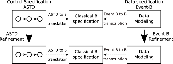
Our approach uses a coupling of the graphical astd notation and Event-B to specify a system. The specification methodology is shown in Fig. 1. A system can be viewed in two parts. The first part models the dynamic behaviour of the system, and is specified in astd (box on the left in Fig. 1). The second part focuses on data, and is described in Event-B (box on the right in Fig. 1). Transitions constitute the link between the two parts: to each action label in astd corresponds an event in Event-B. To ensure the global consistency of the system, the astd and Event-B specifications are translated into classical B (middle box in Fig. 1). As we will explain later, the classical B is only used for technical reasons.
3.1 astd specification.
With graphical notations and process algebra operators, an astd specification models the ordering of actions. Since formal notations are not always easy to understand, astd provides a graphical visualisation which makes the model validation easier, while still remaining formal. Compared to Statecharts, the astd language is based on process algebra operators, like quantified parameterised synchronisation, which allows to represent many processes in parallel.
3.2 Event-B specification.
Event-B specification contains an event for each action label declared in astd. The astd part just describes the ordering of actions. In the Event-B part we specify the effects on the data model of each astd action. Static properties like safety and typing constraints are specified by means of Event-B invariants. Sometimes we need temporal properties which are not supported by the Event-B notation. In that case, we encode these temporal properties by using theorems. Rodin tools are used to generate and prove the proof obligations associated to invariant preservation and additional theorems.
3.3 B specification.
The classical B specification contains two B machines. The first one is the translation of the astd specification, the second one is a transcription of the Event-B specification.
The astd to B translation can be summed up as follows. astd states are encoded by B state variables. To every astd action label corresponds a B operation. Its precondition checks that the state variable is in the initial state of the astd transition. Its postcondition assigns to the state variable the final state of the transition. Moreover, to link the resulting B operation with the data model, we would like to execute the events defined in the Event-B part during the transition. But technically, a B operation cannot call an Event-B event. That is why we also have to translate the events into B operations.
For the translation of the Event-B machine, variables and typing invariants remain unchanged. Events are rewritten into B operations: their guards are simply changed into preconditions and their postconditions remain identical. Grouping the two parts together in one unique B specification allows the global consistency (one horizontal level in Fig. 1) of the system to be proved: when we call an operation in B, the generated proof obligation checks that the precondition of the called operation is true before executing it. To prove the calling proof obligations, invariants are added in the B machine that is the translation of the astd. These invariants link the variables of the Event-B description and the variables that encode the states of the astd.
Event-B provides the expressiveness and the refinement relation required for the system to be modelled, but it lacks some modularity features. There exist theoretical foundations for modularity in Event-B [19], but in practice, they are not yet supported by existing tools. B is then used for technical reasons.
3.4 Refinement of the model.
The methodology uses two refinements. On one side we refine the astd specification (left refinement arrow in Fig. 1), on the other side we refine the data specification in Event-B (right refinement arrow in Fig. 1).
A first definition of astd refinement is proposed in [14]. This refinement definition requires the traces to be preserved and three generic application patterns are described. By trying to apply this astd refinement relation on the case study described here, we realise that it is too restrictive. Consequently we have introduced new patterns that weaken the original definition but preserve behaviour consistency: the properties that are true in a state of the abstract astd specification have to be preserved in the corresponding state of the concrete specification. This new refinement definition is detailed in section 4.4.
The Event-B part of the specification is refined using Event-B definition of refinement. The proof obligations are automatically generated by the RODIN tool. The Event-B refinement guarantees the preservation of the invariants in the data specification. This refinement definition is one of the reasons why we chose Event-B to specify the data part of the system: The classical B refinement does not allow events to be added, while astd refinement allows new transitions.
4 Case Study
Our Event-B/astd coupling is used to specify a train system, more precisely a CBTC-like train controller. CBTC is an automatic train control system based on communications between two subsystems. The track controller manages the entire track where the trains are moving. An on-board controller drives each train. At the most abstract level, the specification consists of trains moving independently. The aim is to define a two-part-system: a part of the system drives the trains, another part manages all the trains on the track. Informally, the property we want to prove for the system is the absence of collision.
Using formal methods to specify railway systems has already been done in the litterature. Ferrari and al. [12] use semi-formal methods to specify a complete CBTC specification. They define a methodology in a software product line approach. Many articles describe the use of formal methods to specify interlocking system: Abrial specifies it with Event-B in the Event-B book [2], James et al. with CSPB [20]. Silva uses Event-B too to specify a train system in his PhD thesis [27]. Our specification starts from a more abstract global view of the system and we refine it into the specification of two controllers. The other approaches directly specify the behaviour of each controller, without considering their global composition as we do.
4.1 Modelling Choices
At the most abstract level, we consider a unique track on which a set of trains are moving in the same direction. This is realistic since, if there are trains in the opposite direction, they are blocked at switches. Furthermore, all issues concerning switches, interlocking, etc… are not considered in this paper. They can be dealt with in subsequent refinement steps. Consequently, we check only the absence of front-to-rear collision
We define a set named on which there is a total, strict order relation (irreflexive, transitive and asymetric) called . means that the element is behind the element on the track.
In the following, we present four levels of specification. In the first one, the trains are moving independently, the second one introduces a controller for each train, the third one groups the controllers together into one single control operation and the last one splits the variables between two entities, preparing for the decomposition.
4.2 First Specification
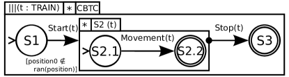
We start by specifying the system behaviour in astd (in Fig. 2). The fact that we have many trains is represented by the quantified interleaving operator. Each train can start, move and stop. is an astd of type Kleene closure: this means that the body of (i.e. the transition) can be performed zero, one or more times. When it is stopped, a train can restart thanks to the Kleene closure.
Since we assume that the trains are moving in the same direction on one track, the non-collision property can be expressed by two predicates:
| (1) |
Predicate (4.2) means that the position of two distinct trains are different. Another predicate is needed to express that a train cannot jump over another train.
| (2) |
Predicate (4.2) checks that the order of trains does not change. Symbol denotes the ”next” operator from temporal logic [23].
To express these predicates in Event-B we introduce a set and a state variable which is a partial function from to (). Variable is set when the train starts and until it stops. The EventB event, corresponding to the movement action, that acts on the data is called . It updates the variable such as (see Figure 3):
-
•
the new position is different from the positions of the other trains;
-
•
the new position stays behind the position of the trains that were located before;
-
•
the new position cannot be located behind the old position.
- Event
-
movement_act
- any
-
-
- where
-
-
gu1 :
-
gu2 :
-
- then
-
-
act1 :
-
- end
Predicate (4.2) is directly defined as an invariant of the data specification. Predicate (4.2) uses an operator coming from temporal logic and cannot be model checked by ProB. To avoid this issue, we translate temporal logic predicate (4.2) into assertions on the states, written as Event-B theorems. An Event-B theorem is an assertion that has to be proved with the invariants of the machine. A theorem is written for each event of the machine. For example, the theorem corresponding to the event checks that for all trains , and such that , (a) if is behind , (b) if the precondition of the operation is true for , (c) if we execute then stays behind . Note that this theorem includes the three possible cases: , and ( and )
astd and Event-B specification are then translated into classical B. We detail the example of the action label. In the astd translation, a operation is created. The precondition of the operation verifies that the state variable is the initial state of the precondition (state 2.1 of astd in Fig. 2). The postcondition assigns the final state of the transition to the state variable (state 2.2 of astd in Fig. 2) and calls the translation of the Event-B operation. The operation is
The translation of operation is
| END |
where is the same predicate as in the act1 part of the Event-B postcondition of .
In the data specification we have already proved that the invariant is preserved if the guards of the events are true. In the unifying machine, generated proof obligations require to prove the precondition (hence the guard of the event) of the called operation () to be true when the operation is called (i.e. ). These two proofs imply that the invariant is always preserved. This justifies the need of a unifying machine for proving the horizontal consistency.
4.3 First Refinement
At the abstract level, the operation describes the properties that the new position must satisfy. In this refinement, we show how such a position can be chosen. A computing operation is added for each train. It computes a limit for the train, called (Movement Authority Limit), given all the positions of the other trains. The operation now updates the position such that the train cannot overtake the limit.
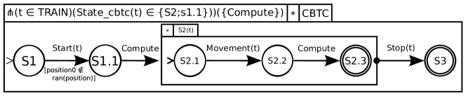
In the astd specification, the action label that computes the limit is added twice. Just after a train starts, the system computes a . Each time a train has moved, the system has to compute a new . The new ASTD specification is in Fig. 4. The refinement is proved using the refinement definition given in [14].

Since a new action label is added in the astd, we need to describe its effects on the data model in Event-B. It computes a limit for the train. This limit is the variable of the Event-B specification. The invariant properties associated to are:
| (3) |
| (4) |
Predicate (4.3) checks that the of a train is always located behind the trains that are in front of it. Predicate (4) checks that a train cannot overtake its limit.
The operation (see Figure 5) computes the limit for a train such that: (a) the new is in front of or equal to current , (b) for all trains whose is in front of , the new is behind .
- Event
-
compute_l_act
- any
-
-
- where
-
-
gu1 :
-
gu2 :
-
- then
-
-
act1 :
-
- end
Since we compute limit for the trains, we modify the operation (Figure 6) such that the new position of a train is chosen depending on : the new position is between the old and .
- Event
-
movement_act
- refines
-
movement_act
- any
-
-
- where
-
-
gu1 :
-
gu2 :
-
gu3 :
-
- then
-
-
act1 :
-
- end
4.4 Second Refinement
In this level of refinement, all the local computing operations are grouped into one global operation. It is synchronised for all the started trains ( operator). The new specification is depicted in Fig. 7.
This refinement transforms an interleaving astd into a synchronised astd . The set of accepted traces is restricted. But we want to preserve behaviour consistency: For each train the astd is a refinement of the astd according to the definition proposed in [14]. It means that if the global set of traces accepted by the astd specification is reduced, the local behaviour of each entities is preserved.
Since we change the local operation into a global one, we need to define this operation in the data specification. This operation computes for all trains a limit such that the limit respects the invariants defined in section 4.3. The specification of is shown on Figure 8.
- Event
-
compute_act
- begin
-
-
act1 :
-
- end
Proving this refinement is not possible in Event-B: a set of local events cannot be refined by a global one. To prove the consistency of our specification, we proved that executing operation is equivalent to execute any sequence of (which means an interleaving of ).
To prove the refinement, events are expressed as relations between the state of a variable before and after executing the event. We write the relation for an event and if the event has a parameter. We proved that (a) for all and , and being in , which means that for all couples of trains, the order in which we execute event does not change the result. Using (a) and by induction on the set of trains, we proved that all the sequences of execution are equivalent. Finally, we proved that executing an arbitrary sequence of is equivalent to execute . This implies that executing is equivalent to execute an interleaving of event.
4.5 Third Refinement
We want our system to have two subsystems. The on-board system drives the trains. It modifies variable , using variable . The track system manages the entire subsystem. It computes variable using variable . To share the variables between two subsystems, communications are introduced.
Each variable of the second refinement is refined by two variables: one variable called track variable is used and modified by the track controller and the other one called on-board variable is used and modified by the on-board controller. The gluing invariant is .
In the data specification, variable is replaced by in the operations that modifies it, and variable is replaced by . The rest of the specification remains almost unchanged: some guards are added to prove the Event-B refinement. A communication operation (resp. ) send variable (resp. ) from the board to the track (resp. from the track to the board). The specification of the is shown in Figure 9
- Event
-
commBT_act
- any
-
-
- where
-
-
gu1 :
-
gu2 :
-
- then
-
-
act1 :
-
- end
In the control specification, after each operation that modifies variable (the operation and ), a communication operation from the board to the track () is added. Dually, a communication operation from the track to the board () is added after the operation. The astd specification can be seen in Figure 10.
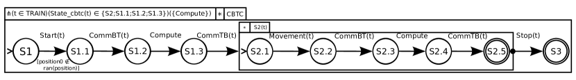
The astd refinement follows the refinement definition of [14]. The refinement of the data specification follows the Event-B definition of the refinement.
4.6 Discussion about the specification
In this section, we want to evaluate the efficency of our specification method. For this purpose, a benchmark specification was specified. First, we sum up our case study. Then the benchmark specification is explained. Finally, the specifications are compared.
Summary of the case study
In this paper, four levels of specification are presented out of six in the entire case study. The rest of the case study is described in a technical report [11]. The table in Figure 11 sums up the statistics of this case study. It contains the number of lines of specification and the number of proof obligations. The specifications presented in this paper are level 2 to 5. Our aim is to evaluate the efficiency of the astd langage. Thus we only present the statistics about the control specification. The second column is the number of lines in the generated B specification. The last four columns are the number of generated proof obligations. The first column is the total number of proof obligations, the second and third ones are respectivelly the number of automatically and manually proved obligations. The Atelier B tool allows one to save the user proof tactics. Since some proof obligations are similar, some tactics can prove many proof obligations. The last column contains the number of proof tactics that are sufficient to prove all proof obligations.
| Specification Level | Number of lines: Generated B Specification | Number of Proof Obligations | |||||||
|---|---|---|---|---|---|---|---|---|---|
| Total |
|
|
|
||||||
| Level 1 | 98 | 30 | 25 | 5 | 5 | ||||
| Level 2 | 145 | 265 | 225 | 40 | 4 | ||||
| Level 3 | 185 | 342 | 252 | 90 | 14 | ||||
| Level 4 | 201 | 391 | 239 | 152 | 15 | ||||
| Level 5 | 277 | 871 | 337 | 534 | 58 | ||||
|
121 | 149 | 16 | 133 | 13 | ||||
| Level 6 | 422 | 2710 | 1989 | 721 | 60 | ||||
The benchmark specification
To see the advantages and drawbacks of our methodology, a benchmark B specification was written following the traditional development process. This benchmark specification is a specification of the control specification that we have manually derived from the astd specification. The astd specification is used as a user requirement.
One state variable is added for each transition label of the astd specification. This state variable contains the instance of trains for which the transition is enabled. The precondition of an operation verifies if the transition is enabled. The post condition removes the instance for the disabled operations, and adds it for the enable operation. For example, the operation is shown in Figure 12. It means that the transition can be executed for the train if it is in the set . After this operation, neither nor operations are enabled, becomes enabled. The benchmark specification contains 121 lines and generates 149 proof obligations, 133 are proved manually with 13 user tactics.
| PRE | ||
| THEN | ||
Comparison and discussion
We compare the level 5 of our case study with the benchmark specification. Level 5 required to manually prove 534 obligations which were discharged with 58 tactics. The benchmark specification is shorter (121 lines vs 277) and generates less proof obligations (149 vs 871, 13 tactics required vs 58) than our specification. This comes from the fact that the control specification is automatically generated. As a comparison, the Movement operation in the generated B code contains 4 levels of SELECT substitution, which generate a lot of different proof cases. The specification of this operation is not given here for the sake of concision; it is about 30 lines long.
On one hand, the benchmark specification is shorter and easier to prove, but it is almost impossible to be sure it respects the behaviour of the astd specification without proving it. On the other hand, the astd/B specification is automatically translated from the astd specification: thus we are sure it respects the astd specification but the resulting specification is a little hard to prove. We also try to prove the equivalence between the astd/B specification and the benchmark specification. This proof is about as hard as proving the entire astd/B specification, and mistakes were found which shows the necessity of the proof of equivalence.
This comparison provides some evidence that the astd langage is a good, formal and easy to read langage to express user requirements. It can be used in a formal specification methodology, but the resulting specification is hard to prove and a little complex. In the future, we plan to improve the specification methodology to reduce the complexity of the generating specification and to help the user with the proof work.
5 Conclusion
5.1 Related work.
There exist several methods that combine state-based specifications with process algebras. In csp2B [7], a CSP specification is translated into a B machine. Only a subset of CSP operators are allowed for semantics reasons and there are some restrictions on the use of synchronisation and interleaving operators. Contrary to our approach, the basic idea of csp2B is to use one of the two languages (e.g. B) as a central support for verification and refinement.
CSP B [28, 25] consists in associating B machines with CSP controllers, such that B operations are constrained by the CSP process. Communications between B machines are modelled through their respective CSP controllers. The approach provides the sufficient conditions to verify the consistency of the whole specification. This work is probably the closest to our approach. Intrinsically, the decomposition of the system into several pairs B machine/CSP controller implies a clear separation between data model and behavioural description. However, it also induces a very constrained organisation of the model, which may be not straightforward for some systems. Moreover, compared to astd, expressiveness of CSP controllers is limited (see [13] for a comparison between astd and CSP).
Circus [29, 22] is a formal language based on Z [8] and CSP, which integrates the refinement calculus of [4]. The semantics is inspired by the unifying theory of programming [18]. The key idea is to distinguish state transitions from the communications of the main action system that represents the behaviour of the system. CSP roughly offers the same process algebra as astd but without a graphical view. Moreover our data refinement is based on Event-B.
Finally iUML-B combines Event-B with UML. A state machine or a class diagram can be added to an Event-B machine. Those diagrams are translated into Event-B specifications. It does not support the quantified synchronisation that is needed in our case study. Moreover, there is no formal semantics for now.
Let us now focus on refinement. Introducing extra operations is one of the main issues. Event-B refinement [2] allows that, as opposed to classical B. In several event-based formal languages like CSP, a denotational semantics is defined [24]: refinement is then based on inclusions of sets representing observations of the system behaviour. The simplest observation is to consider all the sequences of operations that the system can perform; this corresponds to the traces model. Contrary to astd refinement, such an inclusion of sets of traces allows loss of traces during refinement. Moreover, this semantics does not allow new operations to be added. There are also some minor differences in the other observation models (failures, divergences) such that astd allows definition of extra operations during refinement (see [14] for a more detailed comparison between CSP and astd refinements). Several work [9, 26, 5] deal with the consequences of the introduction of extra operations on the CSP, B or Z refinement semantics. Compatibility in such couplings requires observations on the input/output operations in the models used for refinement. This is consistent with respect to the astd refinement definition.
5.2 Lessons learnt and perspectives.
Our main objective is to formalise the process of transforming informal, high-level user requirements into a global abstract formal specification by stepwise refinement, as advocated in the Event-B method. Through a railway CBTC-like case study, we have shown how to model with two complementary formal languages, e.g. astd and Event-B. Then, we have explored the complementarity and consistency between astd and B-like refinements.
By adopting a specification in two parts, there is a clear separation between data aspects and behavioural description. The refinement steps illustrated in the case study show the interest of considering both refinements. For instance, the first refinement step is astd-oriented and brings more details in the event ordering for describing a specific process. When the state space must be updated, then the Event-B part will be refined. Such refinements are focused on one part of the model, and the idea is to propagate on the other part when some extra specifications are required (e.g. when a new event is inserted in an astd, then it must be defined by means of Event-B substitutions).
An interesting refinement is illustrated by the second refinement step. It corresponds to a joint refinement of both parts of the model. Not only several actions are put together to form a new one (a kind of merge) which is consistent in terms of postcondition, but the main behaviour is modified such that this new action becomes a synchronisation barrier for the different trains, thus implying a behavioural refinement.
We now aim at generalising all these lessons learnt in order to define a complete methodology, that generates a readable and more easily provable specification. The development of supporting tools is work in progress.
References
- [1]
- [2] J. R. Abrial (2007): The Event-B Book. Cambridge Univ. Press, Cambridge.
- [3] Jean-Raymond Abrial (1996): The B-book: assigning programs to meanings. Cambridge Univ. Press, Cambridge, 10.1017/CBO9780511624162.
- [4] R.J. Back & J. von Wright (1998): Refinement Calculus: A Systematic Introduction. Graduate Texts in Computer Science, Springer-Verlag, 10.1007/978-1-4612-1674-2.
- [5] Eerke A. Boiten (2014): Introducing extra operations in refinement. Formal Asp. Comput. 26(2), pp. 305–317. Available at http://dx.doi.org/10.1007/s00165-012-0266-z.
- [6] T. Bolognesi & E. Brinksma (1987): Introduction to the ISO Specification Language LOTOS. Computer Networks and ISDN Systems 14(1), pp. 25–59, 10.1016/0169-7552(87)90085-7.
- [7] M. Butler (1999): csp2B : A Practical Approach to Combining CSP and B. In: FM’99, LNCS 1708, Springer-Verlag, Toulouse, France, pp. 490–508, 10.1007/3-540-48119-2_28.
- [8] J. Davies & J.C.P. Woodcock (1996): Using Z: Specification, Refinement, and Proof. Prentice-Hall.
- [9] John Derrick & Heike Wehrheim (2005): Non-atomic Refinement in Z and CSP. In: ZB 2005: Formal Specification and Development in Z and B, 4th International Conference of B and Z Users, LNCS 3455, Springer-Verlag, Guildford, UK, pp. 24–44. Available at http://dx.doi.org/10.1007/11415787_3.
- [10] M. Embe Jiague, M. Frappier, F. Gervais, P. Konopacki, J. Milhau, R. Laleau & R. St-Denis (2010): Model-Driven Engineering of Functional Security Policies. In: International Conference on Enterprise Information Systems, 3, pp. 374–379.
- [11] T. Fayolle (2014): Specifying a Train System Using ASTD and the B Method. Technical Report. Available at www.lacl.fr/~tfayolle. Http://www.lacl.fr/~tfayolle.
- [12] Alessio Ferrari, GiorgioO. Spagnolo, Giacomo Martelli & Simone Menabeni (2014): From commercial documents to system requirements: an approach for the engineering of novel CBTC solutions. International Journal on Software Tools for Technology Transfer, pp. 1–21. Available at http://dx.doi.org/10.1007/s10009-013-0298-6.
- [13] M. Frappier, F. Gervais, R. Laleau, B. Fraikin & R. St-Denis (2008): Extending Statecharts with Process Algebra Operators. Innovations in Systems and Software Engineering 4(3), pp. 285–292, 10.1007/s11334-008-0064-1.
- [14] M. Frappier, F. Gervais, R. Laleau & J. Milhau (2014): Refinement patterns for ASTDs. Formal Aspects of Computing 26(5), pp. 919–941, 10.1007/s00165-013-0286-3.
- [15] Marc Frappier, Frédéric Gervais, Régine Laleau & Benoît Fraikin (2008): Algebraic State Transition Diagrams. Technical Report, Université de Sherbrooke.
- [16] D. Harel (1987): Statecharts: A Visual Formalism for Complex Systems. Science of Computer Programming 8, pp. 231–274, 10.1016/0167-6423(87)90035-9.
- [17] C.A.R. Hoare (1985): Communicating Sequential Processes. Prentice-Hall.
- [18] C.A.R. Hoare & H. Jifeng (1998): Unifying Theories of Programming. Prentice-Hall.
- [19] Alexei Iliasov, Elena Troubitsyna, Linas Laibinis, Alexander Romanovsky, Kimmo Varpaaniemi, Dubravka Ilic & Timo Latvala (2010): Supporting Reuse in Event B Development: Modularisation Approach. In: Abstract State Machines, Alloy, B and Z, Second International Conference, ABZ 2010, LNCS 5977, Springer-Verlag, pp. 174–188. Available at http://dx.doi.org/10.1007/978-3-642-11811-1_14.
- [20] Philip James, Faron Moller, Hoang Nga Nguyen, Markus Roggenbach, Steve Schneider, Helen Treharne, Matthew Trumble & David Williams (2013): Verification of Scheme Plans using CSPB. In: Towards a Formal Methods Body of Knowledge for Railway Control and Safety Systems, pp. 14–20, 10.1007/978-3-319-05032-4_15. Available at http://orbit.dtu.dk/fedora/objects/orbit:125733/datastreams/file_555e08e8-0922-4f67-80f1-77cca11b5030/content#page=16.
- [21] J. Milhau, A. Idani, R. Laleau, M. Labiadh, Y. Ledru & M. Frappier (2011): Combining UML, ASTD and B for the formal specification of an access control filter. Innovations in Systems and Software Engineering 7(4), pp. 303–313, 10.1007/s11334-011-0166-z.
- [22] MVM Oliveira (2005): A refinement calculus for Circus. Ph.D. thesis, Department of Computer Science, The University of York.
- [23] A. Pnueli (1981): The Temporal Semantics of Concurrent Programs. Theoretical Computer Science 13, pp. 45–60, 10.1016/0304-3975(81)90110-9.
- [24] A.W. Roscoe (1997): The Theory and Practice of Concurrency. Prentice-Hall.
- [25] Steve Schneider & Helen Treharne (2005): CSP theorems for communicating B machines. Formal Asp. Comput. 17(4), pp. 390–422. Available at http://dx.doi.org/10.1007/s00165-005-0076-7.
- [26] Steve Schneider & Helen Treharne (2011): Changing system interfaces consistently: A new refinement strategy for CSPB. Sci. Comput. Program. 76(10), pp. 837–860. Available at http://dx.doi.org/10.1016/j.scico.2010.08.001.
- [27] Renato Silva (2012): Thesis, chapter Chapter 6 : Case Study, pp. 121–160.
- [28] H. Treharne & S. Schneider (1999): Using a Process Algebra to Control B operations. In: IFM’99, Springer-Verlag, York, United Kingdom, pp. 437–457, 10.1007/978-1-4471-0851-1_23.
- [29] J.C.P. Woodcock & A.L.C. Cavalcanti (2002): The Semantics of Circus. In: ZB 2002, LNCS 2272, Springer-Verlag, Grenoble, France, pp. 184–203, 10.1007/3-540-45648-1_10.