Approximate Nonparametric Maximum Likelihood for Mixture Models: A Convex Optimization Approach to Fitting Arbitrary Multivariate Mixing Distributions

Abstract

Nonparametric maximum likelihood (NPML) for mixture models is a technique for estimating mixing distributions that has a long and rich history in statistics going back to the 1950s, and is closely related to empirical Bayes methods. Historically, NPML-based methods have been considered to be relatively impractical because of computational and theoretical obstacles. However, recent work focusing on approximate NPML methods suggests that these methods may have great promise for a variety of modern applications. Building on this recent work, a class of flexible, scalable, and easy to implement approximate NPML methods is studied for problems with multivariate mixing distributions. Concrete guidance on implementing these methods is provided, with theoretical and empirical support; topics covered include identifying the support set of the mixing distribution, and comparing algorithms (across a variety of metrics) for solving the simple convex optimization problem at the core of the approximate NPML problem. Additionally, three diverse real data applications are studied to illustrate the methods’ performance: (i) A baseball data analysis (a classical example for empirical Bayes methods), (ii) high-dimensional microarray classification, and (iii) online prediction of blood-glucose density for diabetes patients. Among other things, the empirical results demonstrate the relative effectiveness of using multivariate (as opposed to univariate) mixing distributions for NPML-based approaches.

1 Introduction

Consider a setting where we have iid observations from a mixture model. More specifically, let $G_{0}$ be a probability distribution on $\mathcal{T}\subseteq{{\mathbb{R}}}^{d}$ and let $\{F_{0}(\cdot\mid\theta)\}_{\theta\in\mathcal{T}}$ be a family of probability distributions on ${{\mathbb{R}}}^{n}$ indexed by the parameter $\theta\in\mathcal{T}$. Throughout the paper, we assume that $\mathcal{T}$ is closed and convex. Assume that $X_{1},...,X_{p}\in{{\mathbb{R}}}^{n}$ are observed iid random variables and that $\Theta_{1},...,\Theta_{p}\in{{\mathbb{R}}}^{d}$ are corresponding iid latent variables, which satisfy

$$X_{j}\mid\Theta_{j}\sim F_{0}(\cdot\mid\Theta_{j})\mbox{ and }\Theta_{j}\sim G_{0}.$$ (1)

In (1), it may be the case that $F_{0}(\cdot\mid\theta)$ and $G_{0}$ are both known (pre-specified) distributions; more frequently, this is not the case. In this paper, we will study problems where the mixing distribution $G_{0}$ is unknown, but will assume $F_{0}(\cdot\mid\theta)$ is known throughout. Problems like this arise in applications throughout statistics, and various solutions have been proposed. The distribution $G_{0}$ can be modeled parametrically, which leads to hierarchical modeling and parametric empirical Bayes methods (e.g. Efron, 2010). Another approach is to model $G_{0}$ as a discrete distribution supported on finitely- or infinitely-many points; this leads to the study of finite mixture models or nonparametric Bayes, respectively (McLachlan and Peel, 2004; Ferguson, 1973). This paper focuses on another method for estimating $G_{0}$: Nonparametric maximum likelihood.

Nonparametric maximum likelihood (NPML) methods for mixture models — and closely related empirical Bayes methods — have been studied in statistics since the 1950s (Robbins, 1950; Kiefer and Wolfowitz, 1956; Robbins, 1956). They make virtually no assumptions on the mixing distribution $G_{0}$ and provide an elegant approach to problems like (1). The general strategy is to first find the nonparametric maximum likelihood estimator (NPMLE) for $G_{0}$, denoted by $\hat{G}$, then perform inference via empirical Bayes (Robbins, 1956; Efron, 2010); that is, inference in (1) is conducted via the posterior distribution $\Theta_{j}\mid X_{j}$, under the assumption $G_{0}=\hat{G}$. Research into NPMLEs for mixture models has included work on algorithms for computing NPMLEs and theoretical work on their statistical properties (e.g. Laird, 1978; Böhning et al., 1992; Lindsay, 1995; Ghosal and van der Vaart, 2001; Jiang and Zhang, 2009). However, implementing and analyzing NPMLEs for mixture models has historically been considered very challenging (e.g. p. 571 of DasGupta, 2008; Donoho and Reeves, 2013). In this paper, we study a computationally convenient approach involving approximate NPMLEs, which sidesteps many of these difficulties and is shown to be effective in a variety of applications.

Our approach is largely motivated by recent work initiated by Koenker and Mizera (2014) and further pursued by others, including Gu and Koenker (2016, 2017a, 2017b) and Dicker and Zhao (2016). Koenker & Mizera studied convex approximations to NPMLEs for mixture models in relatively large-scale problems, with up to 100,000s of observations. In Koenker and Mizera (2014), they showed that for the Gaussian location model, where $X_{j}=\Theta_{j}+Z_{j}\in{{\mathbb{R}}}$ and $\Theta_{j}\sim G_{0}$, $Z_{j}\sim N(0,1)$ are independent, a good approximation to the NPMLE for $G_{0}$ can be accurately and rapidly computed using generic interior point methods.

Koenker and Mizera (2014)’s focus on convexity and scalability is one of the key concepts for this paper. Here, we show how a simple convex approximation to the NPMLE can be used effectively in a broad range of problems with nonparametric mixture models; including problems involving (i) multivariate mixing distributions, (ii) discrete data, (iii) high-dimensional classification, and (iv) state-space models. Backed by new theoretical and empirical results, we provide concrete guidance for efficiently and reliably computing approximate multivariate NPMLEs. Our main theoretical result (Proposition 1) suggests a simple procedure for finding the support set of the estimated mixing distribution. Many of our empirical results highlight the benefits of using multivariate mixing distributions with correlated components (Sections 6.2, 7, and 8), as opposed to univariate mixing distributions, which have been the primary focus of previous research in this area (notable exceptions include theoretical work on the Gaussian location-scale model in Ghosal and van der Vaart (2001) and applications in Gu and Koenker (2017a, b) involving estimation problems with Gaussian models). In Sections 7–9, we illustrate the performance of the methods described here in real-data applications involving baseball, cancer microarray data, and online blood-glucose monitoring for diabetes patients. In comparison with other recent work on NPMLEs for mixture models, this paper distinguishes itself from Gu and Koenker (2016) in that it focuses on more practical aspects of fitting general multivariate NPMLEs. Additionally, in this paper we consider a substantially broader swath of applications than Gu and Koenker (2017a, b) and Dicker and Zhao (2016), where the focus is estimation in Gaussian models and classification with a univariate NPMLE, respectively, and show that the same fundamental ideas may be effectively applied in all of these settings.

2 NPMLEs for mixture models via convex optimization

2.1 NPMLEs

Let ${\mathbb{G}}_{\mathcal{T}}$ denote the class of all probability distributions on $\mathcal{T}\subseteq{{\mathbb{R}}}^{d}$ and suppose that $f_{0}(\cdot\mid\theta)$ is the probability density corresponding to $F_{0}(\cdot\mid\theta)$ (with respect to some given base measure). For $G\in{\mathbb{G}}_{\mathcal{T}}$, the (negative) log-likelihood given the data $X_{1},...,X_{p}$ is

$$\ell(G)=-\frac{1}{p}\sum_{j=1}^{p}\log\left\{\int_{\mathcal{T}}f_{0}(X_{j}\mid\theta)\ dG(\theta)\right\}.$$

The Kiefer-Wolfowitz NPMLE for $G_{0}$ (Kiefer and Wolfowitz, 1956), denoted $\hat{G}$, solves the optimization problem

$$\min_{G\in{\mathbb{G}}_{\mathcal{T}}}\ell(G);$$ (2)

in other words, $\ell(\hat{G})=\min_{G\in{\mathbb{G}}_{\mathcal{T}}}\ell(G)$.

Solving (2) and studying properties of $\hat{G}$ forms the basis for basically all of the existing research into NPMLEs for mixture models (including this paper). Two important observations have had significant but somewhat countervailing effects on this research:

• The optimization problem (2) is convex;

• If $f_{0}(X_{j}|\theta)$ and $\mathcal{T}$ satisfy certain (relatively weak) regularity conditions, then $\hat{G}$ exists and may be chosen so that it is a discrete measure supported on at most $p$ points.

The first observation above is obvious; the second summarizes Theorems 18–21 of Lindsay (1995). Among the more significant regularity conditions mentioned in (ii) is that the set $\{f_{0}(X_{j}|\theta)\}_{\theta\in\mathcal{T}}$ should be bounded for each $j=1,...,p$.

Observation (i) leads to KKT-like conditions that characterize $\hat{G}$ in terms of the gradient of $\ell$ and can be used to develop algorithms for solving (2) (e.g. Lindsay, 1995). While this approach is somewhat appealing, (2) is typically an infinite-dimensional optimization problem (whenever $\mathcal{T}$ is infinite). Hence, there are infinitely many KKT conditions to check, which is generally impossible in practice.

On the other hand, observation (ii) reduces (2) to a finite-dimensional optimization problem. Indeed, (ii) implies that $\hat{G}$ can be found by restricting attention in (2) to $G\in{\mathbb{G}}_{p}$, where ${\mathbb{G}}_{p}$ is the set of discrete probability measures supported on at most $p$ points in $\mathcal{T}$. Thus, finding $\hat{G}$ is reduced to fitting a finite mixture model with at most $p$ components. This is usually done with the EM-algorithm (Laird, 1978), where in practice one may restrict to $G\in{\mathbb{G}}_{q}$ for some $q<p$. More recently, Wang and Wang (2015) proposed to estimate $G$ in a multivariate setting using a gradient based method. However, while (ii) reduces (2) to a finite-dimensional problem, we have lost convexity:

$$\min_{G\in{\mathbb{G}}_{q}}\ell(G)$$ (3)

is not a convex problem because ${\mathbb{G}}_{q}$ is nonconvex. When $q$ is large (and recall that the theory suggests we should take $q=p$), well-known issues related to nonconvexity and finite mixture models become a significant obstacle (McLachlan and Peel, 2004).

2.2 A simple finite-dimensional convex approximation

In this paper, we take a very simple approach to (approximately) solving (2), which maintains convexity and immediately reduces (2) to a finite-dimensional problem. Consider a pre-specified finite grid $\Lambda\subseteq\mathcal{T}$. We study estimators $\hat{G}_{\Lambda}$, which solve

$$\min_{G\in{\mathbb{G}}_{\Lambda}}\ell(G).$$ (4)

The key difference between (3) and (4) is that ${\mathbb{G}}_{\Lambda}$, and hence (4), is convex, while ${\mathbb{G}}_{q}$ is nonconvex. Additionally, (4) is a finite-dimensional optimization problem, because $\Lambda$ is finite.

To derive a more convenient formulation of (4), suppose that

$$\Lambda=\{t_{1},...,t_{q}\}\subseteq\mathcal{T}$$ (5)

and define the simplex $\Delta^{q-1}=\{w=(w_{1},...,w_{q})\in{{\mathbb{R}}}^{q};\ w_{k}\geq 0,\ w_{1}+\cdots+w_{q}=1\}$. Additionally, let $\delta_{t}$ denote a point mass at $t\in{{\mathbb{R}}}^{d}$. Then there is a correspondence between $G=\sum_{k=1}^{q}w_{k}\delta_{t_{k}}\in\mathcal{G}_{\Lambda}$ and points $w=(w_{1},...,w_{q})\in\Delta^{q-1}$. It follows that (4) is equivalent to the optimization problem over the simplex,

$$\min_{w\in\Delta^{q-1}}-\frac{1}{p}\sum_{j=1}^{p}\log\left\{\sum_{k=1}^{q}f_{0}(X_{j}|t_{k})w_{k}\right\}.$$ (6)

Researchers studying NPMLEs have previously considered estimators like $\hat{G}_{\Lambda}$, which solve (4)–(6). However, most have focused on relatively simple models with univariate mixing distributions $G_{0}$ (Böhning et al., 1992; Jiang and Zhang, 2009; Koenker and Mizera, 2014). In very recent work, Gu and Koenker (2017a, b) have considered multivariate NPMLEs for estimation problems involving Gaussian models — by contrast, our aim is to formulate strategies for solving and implementing the general problem, as specified in (2), (4), and (6).

3 Choosing $\Lambda$

The approximate NPMLE $\hat{G}_{\Lambda}$ is the estimator we use throughout the rest of the paper. One remaining question is: How should $\Lambda$ be chosen? Our perspective is that $\hat{G}_{\Lambda}$ is an approximation to $\hat{G}$ and its performance characteristics are inherited from $\hat{G}$. In general, $\hat{G}_{\Lambda}\neq\hat{G}$. However, as one selects larger and larger finite grids $\Lambda\subseteq\mathcal{T}$, which are more and more dense in $\mathcal{T}$, evidently $\hat{G}_{\Lambda}\to\hat{G}$. Thus, heuristically, as long as the grid $\Lambda$ is “dense enough” in $\mathcal{T}$, $\hat{G}_{\Lambda}$ should perform similarly to $\hat{G}$.

If $\mathcal{T}$ is compact, then any regular grid $\Lambda\subseteq\mathcal{T}$ is finite and implementing (4) is straightforward (specific implementations are discussed in Section 5). Thus, for compact $\mathcal{T}$, one can choose $\Lambda$ to be a regular grid with as many points as are computationally feasible. For general $\mathcal{T}$, we propose a two-step approach to choosing $\Lambda$: (i) Find a compact convex subset $\mathcal{T}_{0}\subseteq\mathcal{T}$ so that (2) is equivalent (or approximately equivalent) to

$$\inf_{G\in\mathcal{G}_{\mathcal{T}_{0}}}\ell(G);$$ (7)

(ii) choose $\Lambda\subseteq\mathcal{T}_{0}\subseteq\mathcal{T}$ to be a regular grid with $q$ points, for some sufficiently large $q$. Empirical results seem to be fairly insensitive to the choice of $q$. In Sections 7–9, we choose $q=30^{d}$ for models with $d=2,3$ dimensional mixing distributions $G$. For some simple models with univariate $G$ ($d=1$), theoretical results suggest that if $q=\sqrt{p}$, then $\hat{G}_{\Lambda}$ is statistically indistinguishable from $\hat{G}$ (Dicker and Zhao, 2016).

Now we form strategies to construct $\Lambda$ for multivariate mixing distribution. First note that Lindsay (1981, 1995) has proposed the construction of $\Lambda$ in one dimensional cases. Our approach may be viewed as a generalization of their work. For each $j=1,\ldots,p$, define

$$\hat{\theta}_{j}=\hat{\theta}(X_{j})=\mathop{\rm arg\,max}_{\theta\in\mathcal{T}}f_{0}(X_{j}\mid\theta)$$

to be the maximum likelihood estimator (MLE) for $\Theta_{j}$, given the data $X_{j}\in{{\mathbb{R}}}^{n}$. The following proposition implies that (2) and (7) are equivalent when the likelihoods $f_{0}(X_{j}\mid\theta)$ are from a class of elliptical unimodal distributions, and $\mathcal{T}_{0}=\mathrm{conv}(\hat{\theta}_{1},\ldots,\hat{\theta}_{p})$ is the convex hull of $\hat{\theta}_{1},\ldots,\hat{\theta}_{p}$. This result enables us to employ the strategy described above for choosing $\Lambda$ and finding $\hat{G}_{\Lambda}$; specifically, we take $\Lambda$ to be a regular grid contained in the compact convex set $\mathrm{conv}(\hat{\theta}_{1},\ldots,\hat{\theta}_{p})$.

Proposition 1.

Suppose that $f_{0}$ has the form

$$f_{0}(X_{j}\mid\theta)=h\big{\{}(\hat{\theta}_{j}-\theta)^{\top}\Sigma^{-1}(\hat{\theta}_{j}-\theta)\big{\}}u(X_{j}),$$ (8)

where $h:[0,\infty)\to[0,\infty)$ is a decreasing function, $\Sigma$ is a $p\times p$ positive definite matrix, and $u:{{\mathbb{R}}}^{n}\to{{\mathbb{R}}}$ is some other function that does not depend on $\theta$. Let $\mathcal{T}_{0}=\mathrm{conv}(\hat{\theta}_{1},\ldots,\hat{\theta}_{p})$. Then $\ell(\hat{G})=\inf_{G\in{\mathbb{G}}_{\mathcal{T}_{0}}}\ell(G)$.

Proof.

Assume that $G=\sum_{k=1}^{q}w_{k}\delta_{t_{k}}$, where $t_{1},\ldots,t_{q}\in\mathcal{T}$ and $w_{1},\ldots,w_{q}>0$. Further assume that $t_{q}\notin\mathcal{T}_{0}=\mathrm{conv}(\hat{\theta}_{1},\ldots,\hat{\theta}_{p})$. We show that there is another probability distribution $\tilde{G}=\sum_{k=1}^{q-1}w_{k}\delta_{t_{k}}+w_{q}\delta_{\tilde{t}_{q}}$, with $\tilde{t}_{q}\in\mathcal{T}_{0}$, satisfying $\ell(\tilde{G})\leq\ell(G)$. This suffices to prove the proposition.

Let $\tilde{t}_{q}$ be the projection of $t_{q}$ onto $\mathcal{T}_{0}$ with respect to the inner product $(s,t)\mapsto s^{\top}\Sigma^{-1}t$. To prove that $\ell(\tilde{G})\leq\ell(G)$, we show that $f_{0}(X_{j}\mid\tilde{t}_{q})\geq f_{0}(X_{j}\mid t_{q})$ for each $j=1,\ldots,p$. We have

$$(\hat{\theta}_{j}-t_{q})^{\top}\Sigma^{-1}(\hat{\theta}_{j}-t_{q}) =(\hat{\theta}_{j}-\tilde{t}_{q}+\tilde{t}_{q}-t_{q})^{\top}\Sigma^{-1}(\hat{\theta}_{j}-\tilde{t}_{q}+\tilde{t}_{q}-t_{q})$$

$$=(\hat{\theta}_{j}-\tilde{t}_{q})^{\top}\Sigma^{-1}(\hat{\theta}_{j}-\tilde{t}_{q})+2(\tilde{t}_{q}-t_{q})^{\top}\Sigma^{-1}(\hat{\theta}_{j}-\tilde{t}_{q})$$

$$\qquad+(\tilde{t}_{q}-t_{q})^{\top}\Sigma^{-1}(\tilde{t}_{q}-t_{q})$$

$$\geq(\hat{\theta}_{j}-\tilde{t}_{q})^{\top}\Sigma^{-1}(\hat{\theta}_{j}-\tilde{t}_{q}),$$

where we have used the fact that $(\tilde{t}_{q}-t_{q})^{\top}\Sigma^{-1}(\hat{\theta}_{j}-\tilde{t}_{q})=0$, because $\tilde{t}_{q}$ is the projection of $t_{q}$ onto $\mathcal{T}_{0}$. By (8), it follows that $f_{0}(X_{j}\mid\tilde{t}_{q})\geq f_{0}(X_{j}\mid t_{q})$, as was to be shown. ∎

The condition (8) is rather restrictive, but we believe it applies in a number of important problems. The fundamental example where (8) holds is $X_{j}\mid\Theta_{j}\sim N(\Theta_{j},\Sigma)$; in this case $\hat{\theta}_{j}=X_{j}$ and (8) holds with $u$ being certain constant and $h(z)\propto e^{-z/2}$. Condition (8) also holds in elliptical models, where $\Theta_{j}$ is the location parameter of $X_{j}\mid\Theta_{j}$. More broadly, if $X_{j}=(X_{1j},\ldots,X_{nj})^{\top}\in{{\mathbb{R}}}^{n}$ may be viewed as a vector of replicates $X_{ij}$, $i=1,\ldots,n$, drawn from some common distribution conditional on $\Theta_{j}$, then standard results suggest that the MLEs $\hat{\theta}_{j}$ may be approximately Gaussian if $n$ is sufficiently large, and (8) may be approximately valid. Specific applications where a normal approximation argument for $\hat{\theta}_{j}$ may imply that (8) is approximately valid include count data (similar to Section 7) and time series modeling (Section 9).

4 Connections with finite mixtures

Finding $\hat{G}_{\Lambda}$ is equivalent to fitting a finite-mixture model, where the locations of the atoms for the mixing measure have been pre-specified (specifically, the atoms are taken to be the points in $\Lambda$). Thus, the approach in this paper reduces computations for the relatively complex nonparametric mixture model (1) to a convex optimization problem that is substantially simpler than fitting a standard finite mixture model (generally a non-convex problem).

An important distinction of nonparametric mixture models is that they lack the built-in interpretability of the components/atoms from finite mixture models, and are less suited for clustering applications. On the other hand, taking the nonparametric approach provides additional flexibility for modeling heterogeneity in applications where it is not clear that there should be well-defined clusters. Moreover, post hoc clustering and finite mixture model methods could still be used after fitting an NPMLE; this might be advisable if, for instance, $\hat{G}_{\Lambda}$ has several clearly-defined modes.

5 Implementation overview

A variety of well-known algorithms are available for solving (6) and finding $\hat{G}_{\Lambda}$. We have experimented with several, including the EM-algorithm, interior point methods, and the Frank-Wolfe algorithm. This section contains a brief overview of how we have implemented these algorithms; numerical results comparing the algorithms are contained in the following section.

One of the early applications of the EM-algorithm is mixture models (Laird, 1978). Solving (6) with the EM-algorithm for mixture models with predetermined grid-points is especially simple, because the problem is convex (recall that the finite mixture model problem — as opposed to the nonparametric problem — is typically non-convex). Koenker and Mizera (2014) have developed interior point methods for solving (6). Along with Koenker and Gu (2016), they created an R package REBayes that solves (6) for a handful of specific nonparametric mixture models, e.g. Gaussian mixtures and univariate Poisson mixtures; the REBayes package calls an external optimization software package, Mosek, and relies on Mosek’s built-in interior point algorithms. In our numerical analyses, we used REBayes to compute some one-dimensional NPMLEs with interior point methods. To estimate multi-dimensional NPMLEs with interior point methods, we used our own implementations based on another R package Rmosek (ApS, 2015) (REBayes does appear to have some built-in functions for estimating two-dimensional NPMLEs, but we found them to be somewhat unstable in our applications). We note that our interior point implementation solves the primal problem (6), while REBayes solves the dual. The Frank-Wolfe algorithm (Frank and Wolfe, 1956) is a classical algorithm for constrained convex optimization problems, which has recently been the subject of renewed attention (e.g. Jaggi, 2013). Our implementation of the Frank-Wolfe algorithm closely resembles the “vertex direction method,” which has previously been used for finding the NPMLE in nonparametric mixture models (Böhning, 1995).

All of the algorithms used in this paper were implemented in R. We did not attempt to heavily optimize any of these implementations; instead, our main objective was to demonstrate that there are a range of simple and effective methods for finding (approximate) NPMLEs. While the REBayes and Rmosek packages were used for their interior point methods, no packages beyond base R were required for any of our other implementations.

6 Simulation studies

This section contains simulation results for NPMLEs and a Gaussian location-scale mixture model. Section 6.1 contains a comparison of the various NPMLE algorithms described in the previous section. In Section 6.2, we compare the performance of NPMLE-based estimators to other commonly used methods for estimating the mean in a Gaussian location-scale model.

In all of the simulations described in this section we generated the data as follows. For $j=1,\ldots,p$, we generated independent $\Theta_{j}=(\mu_{j},\sigma_{j})\sim G_{0}$ and corresponding observations $X_{j}\in{{\mathbb{R}}}^{n}$. Each $X_{j}=(X_{1j},\ldots,X_{nj})^{\top}$ was a vector of $n$ replicates $X_{1j},\ldots,X_{nj}\mid\Theta_{j}\sim N(\mu_{j},\sigma_{j}^{2})$ that were generated independently, conditional on $\Theta_{j}$. In other words,

$$X_{j}\mid\Theta_{j}\sim f_{0}(X_{j}|\Theta_{j})=\left(\frac{1}{\sqrt{2\pi}\sigma_{j}}\right)^{n}\exp\left\{-\frac{\sum_{i=1}^{n}(X_{ij}-\mu_{j})^{2}}{2\sigma_{j}^{2}}\right\}.$$ (9)

In the general model (9), the mixing distribution $G_{0}$ is bivariate. However, we considered two values of $G_{0}$ in our simulations: one where the marginal distribution of $\sigma_{j}$ was degenerate (i.e. $\sigma_{j}$ was constant, so $G_{0}$ was effectively univariate) and one where the marginal distribution of $\sigma_{j}$ was non-degenerate. (Note that for non-degenerate $\sigma_{j}$, $n\geq 2$ replicates are essential in order to ensure that the likelihood is bounded and that $\hat{G}$ exists.)

Throughout the simulations, we took $p=1000$ and $n=16$. For the first mixing distribution $G_{0}$ (degenerate $\sigma_{j}$), we fixed $\sigma_{j}=4$ and took $\mu_{j}$ so that ${\mathbb{P}}(\mu_{j}=0)={\mathbb{P}}(\mu_{j}=5)=1/2$. For the second mixing distribution (non-degenerate $\sigma_{j}$), we took ${\mathbb{P}}(\mu_{j}=0,\ \sigma_{j}=5)={\mathbb{P}}(\mu_{j}=5,\ \sigma_{j}=3)=0.5$; for this distribution $\mu_{j}$ and $\sigma_{j}$ are correlated.

6.1 Comparing NPMLE algorithms

For each mixing distribution, we computed $\hat{G}_{\Lambda}$ using the algorithms described in Section 5: the EM-algorithm, an interior point method with Rmosek, and the Frank-Wolfe algorithm. For each of these algorithms, we also computed $\hat{G}_{\Lambda}$ for various grids $\Lambda$. Specifically, we considered regular grids $\Lambda=\{m_{k}\}_{k=1}^{q_{1}}\times\{s_{k}\}_{k=1}^{q_{2}}\subseteq[\min\hat{\mu}_{j},\max\hat{\mu_{j}}]\times[\min\hat{\sigma}_{j},\max\hat{\sigma}_{j}]\subseteq{{\mathbb{R}}}^{2}$, where $\hat{\mu}_{j}=n^{-1}\sum_{i}X_{ij}$ and $\hat{\sigma}_{j}^{2}=n^{-1}\sum_{i}(X_{ij}-\hat{\mu}_{j})^{2}$. The values $q_{1},q_{2}$ determine number of grid-points in $\Lambda$ for $\mu_{j},\sigma_{j}$, respectively, and in the simulations we fit estimators with $(q_{1},q_{2})=(30,30),(50,50)$, and $(100,100)$. The stopping criterion of EM and Frank-Wolfe is

$$|\ell(w^{(K)})-\ell(w^{K-1})|/|\ell(w^{(K-1)}|\leq 10^{-6},$$

where $\ell(w)$ is the objective function in (6) and $w^{(K)}$ is the solution at the $K$-th iteration of respective methods.

In addition to fitting the two-dimensional NPMLEs $\hat{G}_{\Lambda}$ described above, for the simulations with degenerate $\sigma_{j}$ we also fit one-dimensional NPMLEs to the data $\hat{\mu}_{1},\ldots,\hat{\mu}_{p}$, according to the model

$$\hat{\mu}_{j}\mid\mu_{j}\sim N(\mu_{j},1).$$

We fit these one-dimensional NPMLEs using all of the same algorithms for the two-dimensional NPMLEs (EM, interior point with Rmosek, and Frank-Wolfe), and we also used the REBayes interior point implementation to estimate the distribution of $\mu_{j}$ in this setting. For the one-dimensional NPMLEs, we took $\Lambda\subseteq[\min\hat{\mu}_{j},\max\hat{\mu}_{j}]\subseteq{{\mathbb{R}}}$ to be the regular grid with $q=300$ points. This allows us to compare the performance of methods for one- and two-dimensional NPLMEs (where the one-dimensional NPMLEs take the distribution of $\sigma_{j}$ to be known) and compare the performance of the two interior point algorithms, among other things.

For each simulated dataset and estimator $\hat{G}_{\Lambda}$ we recorded several metrics. First, we computed the total squared error (TSE)

$$\mathrm{TSE}=\sum_{j=1}^{p}(\widehat{\mu}_{j}-\mu_{j})^{2},$$

where

$$\hat{\mu}_{j}={\mathbb{E}}_{\hat{G}_{\Lambda}}(\mu_{j}\mid X_{j})=\frac{\int\mu_{j}f_{0}(X_{j}|\mu_{j},\sigma_{j})d\hat{G}_{\Lambda}(\mu_{j},\sigma_{j})}{\int f_{0}(X_{j}|\mu_{j},\sigma_{j})d\hat{G}_{\Lambda}(\mu_{j},\sigma_{j})}.$$

Second, we computed the difference between the log-likelihood of $\hat{G}_{\Lambda}$ and the log-likelihood of $\hat{G}_{\mathrm{EM}}$, the corresponding estimator for $G_{0}$ based on the EM-algorithm:

$$\Delta(\mbox{log-lik.})=\ell(\hat{G}_{\mathrm{EM}})-\ell(\hat{G}_{\Lambda}).$$

Note that $\Delta(\mbox{log-lik.})>0$ if $\hat{G}_{\Lambda}$ has a smaller negative log-likelihood than $\hat{G}_{\mathrm{EM}}$ (we are taking the EM-estimator $\hat{G}_{\mathrm{EM}}$ as a baseline for measuring the log-likelihood). Finally, we recorded the time required to compute $\hat{G}_{\Lambda}$ (in seconds; all calculations were performed on a 2015 MacBook Pro laptop). Summary statistics are reported in Table 1.

It is evident that the results in Table 1 are relatively insensitive to the number of grid-points $(q_{1},q_{2})$ chosen for the two-dimensional NPMLE implementations. In terms of TSE, the EM algorithm and interior point methods perform very similarly across all of the settings, while the interior point methods appear to slightly out-perform the EM algorithm in terms of $\Delta(\mbox{log-lik.})$ across the board. Additionally, the interior point methods have smaller compute time than the EM algorithm, though the difference is not too significant for applications at this scale (for mixing distribution 1, with degenerate $\sigma_{j}$, the REBayes dual implementation appears to be somewhat faster than our Rmosek primal implementation). The Frank-Wolfe algorithm is the fastest implementation we have considered, but its performance in terms of TSE and $\Delta(\mbox{log-lik.})$ is considerably worse than the EM algorithm or interior point methods. In the remainder of the paper, we chose to use the EM algorithm exclusively for computing NPMLEs — we believe it strikes a balance between simplicity and performance.

Table 1: Comparison of different NPMLE algorithms. Mean values (standard deviation in parentheses) reported from 100 independent datasets; $p=1000$, throughout simulations. Mixing distribution 1 has constant $\sigma_{j}$; mixing distribution 2 has correlated $\mu_{j}$ and $\sigma_{j}$.

		TSE	$\Delta(\text{log-lik})$ $\!\times\!10^{4}$	Time (secs.)
Mixing dist. 1	EM
(Bivariate)	$(q_{1},q_{2})=(30,30)$	130.5 (42.6)	0 (0)	9
	$(q_{1},q_{2})=(50,50)$	130.4 (42.7)	0 (0)	33
	$(q_{1},q_{2})=(100,100)$	130.4 (42.6)	0 (0)	136
	Interior point (Rmosek)
	$(q_{1},q_{2})=(30,30)$	130.7 (42.6)	6 (1)	8
	$(q_{1},q_{2})=(50,50)$	130.5 (42.9)	9 (1)	20
	$(q_{1},q_{2})=(100,100)$	130.6 (42.8)	11 (1)	80
	Frank-Wolfe
	$(q_{1},q_{2})=(30,30)$	147.3 (45.1)	-234 (130)	5
	$(q_{1},q_{2})=(50,50)$	147.0 (45.9)	-238 (134)	14
	$(q_{1},q_{2})=(100,100)$	146.2 (45.4)	-238 (128)	55
Mixing dist. 1	EM	124.4 (41.6)	0 (0)	1
(univariate; $q=300$;	Interior point (Rmosek)	124.3 (42.1)	6 (1)	3
assume known $\sigma_{j}$)	Interior point (REBayes)	124.3 (42.1)	6 (1)	1
	Frank-Wolfe	126.1 (41.8)	-4 (4)	1
Mixing dist. 2	EM
	$(q_{1},q_{2})=(30,30)$	54.0 (28.4)	0 (0)	9
	$(q_{1},q_{2})=(50,50)$	54.0 (28.9)	0 (0)	34
	$(q_{1},q_{2})=(100,100)$	53.9 (28.8)	0 (0)	141
	Interior point (Rmosek)
	$(q_{1},q_{2})=(30,30)$	54.3 (28.8)	5 (1)	8
	$(q_{1},q_{2})=(50,50)$	54.2 (29.1)	8 (1)	20
	$(q_{1},q_{2})=(100,100)$	54.3 (29.1)	10 (1)	82
	Frank-Wolfe
	$(q_{1},q_{2})=(30,30)$	82.2 (39.3)	-372 (217)	5
	$(q_{1},q_{2})=(50,50)$	83.1 (36.4)	-402 (232)	14
	$(q_{1},q_{2})=(100,100)$	82.0 (37.7)	-396 (240)	56

6.2 Gaussian location-scale mixtures: Other methods for estimating a normal mean vector

Beyond NPMLEs, we also implemented several other methods that are commonly used for estimating the mean vector $\boldsymbol{\mu}=(\mu_{1},\ldots,\mu_{p})^{\top}\in{{\mathbb{R}}}^{p}$ in Gaussian location-scale models and computed the corresponding TSE. Specifically, we considered the fixed-$\Theta_{j}$ MLE, $\boldsymbol{\widehat{\mu}}=(\hat{\mu}_{1},\ldots,\hat{\mu}_{p})^{\top}\in{{\mathbb{R}}}^{p}$; the James-Stein estimator; the heteroscedastic SURE estimator of Xie et al. (2012); and a soft-thresholding estimator. The James-Stein estimator is a classical shrinkage estimator for the Gaussian location model. The version employed here is described in Xie et al. (2012) and is designed for heteroscedastic data. The heteroscedastic SURE estimator is another shrinkage estimator, which was designed to ensure that features with a high noise variance are “shrunk” more than those with a low noise variance. Both the James-Stein estimator and the heteroscedastic SURE estimator depend on the values $\sigma_{j}$. The soft-thresholding estimator takes the form $\hat{\mu}(X)=s_{t}(\hat{\mu}_{j})$, where $t\geq 0$ is a constant and $s_{t}(x)=\mathrm{sign}(x)\max\{|x|-t,0\}$, $x\in{{\mathbb{R}}}$. For soft-thresholding estimators, $t$ was chosen to minimize the TSE. Observe that the James-Stein, SURE, and soft-thresholding estimators all depend on information that is typically not available in practice: the value of $\sigma_{j}$ and the actual TSE. By contrast, the two-dimensional NPMLEs described in the previous sub-section utilize only the observed data $X_{1},\ldots,X_{p}$.

In Table 2, we report the TSE for the different estimators described in this section, along with the TSE for the bivariate NPMLE fit using the EM algorithm. We also fit a univariate NPMLE in this example, where $\sigma_{j}$ was not assumed to be known; instead we used the plug-in estimator $\hat{\sigma}_{j}$ in place of $\sigma_{j}$ and then computed the NPMLE for the distribution of $\mu_{j}$.

Table 2 shows that the NPMLEs dramatically out-perform the alternative estimators in this setting, in terms of TSE. The bivariate NPMLE out-performs the univariate NPMLE under both mixing distributions 1 and 2, but its advantage is especially pronounced under mixing distribution 2, where $\mu_{j}$ and $\sigma_{j}$ are correlated. This highlights the potential advantages of bivariate NPMLEs over univariate approaches in settings with multiple parameters.

Table 2: Mean TSE for various estimators of $\boldsymbol{\mu}\in{{\mathbb{R}}}^{p}$ based on 100 simulated datasets; $p=1000$. $(q_{1},q_{2})$ indicates the grid-points used to fit $\hat{G}_{\Lambda}$.

Method	Mixing dist.1	Mixing dist.2
Fixed-$\Theta_{j}$ MLE	997.0 (48.2)	1059.3 (57.9)
Soft-Thresholding	826.2 (50.0)	793.7 (46.0)
James-Stein	859.7 (43.6)	935.2 (53.0)
SURE	859.7 (43.6)	880.7 (48.1)
Univariate NPMLE $q=300$	170.7 (47.0)	285.4 (63.5)
Bivariate NPMLE $(q_{1},q_{2})=(100,100)$	130.4 (42.6)	53.9 (28.8)

7 Baseball data

Baseball data is a well-established testing ground for empirical Bayes methods (Efron and Morris, 1975). The baseball dataset we analyzed contains the number of at-bats and hits for all of the Major League Baseball players during the 2005 season and has been previously analyzed in a number of papers (Brown, 2008; Jiang and Zhang, 2010; Muralidharan, 2010; Xie et al., 2012). The goal of the analysis is to use the data from the first half of the season to predict each player’s batting average (hits/at-bats) during the second half of the season. Overall, there are 929 players in the baseball dataset; however, following Brown (2008) and others, we restrict attention to the 567 players with more than 10 at-bats during the first half of the season for training and among which 499 players with more than 10 at-bats during the second half of season for prediction. (We follow the other preprocessing steps described in Brown (2008) as well).

Let $A_{j}$ and $H_{j}$ denote the number of at-bats and hits, respectively, for player $j$ during the first half of the season, $j=1,...,567$. We assume that $(A_{j},H_{j})$ follows a Poisson-binomial mixture model, where $A_{j}\mid(\lambda_{j},\pi_{j})\sim\mbox{Poisson}(\lambda_{j})$, $H_{j}\mid(A_{j},\lambda_{j},\pi_{j})\sim\mbox{binomial}(A_{j},\pi_{j})$, and $(\lambda_{j},\pi_{j})\sim G_{0}$. This model has a bivariate mixing distribution $G_{0}$, i.e. $d=2$. In the notation of (1), $X_{j}=(A_{j},H_{j})$, $\Theta_{j}=(\lambda_{j},\pi_{j})$ and

$$f_{0}(X_{j}|\Theta_{j})=f_{0}(A_{j},H_{j}|\lambda_{j},\pi_{j})=\frac{\lambda_{j}^{A_{j}}e^{-\lambda_{j}}}{A_{j}!}\times{{A_{j}}\choose{H_{j}}}\pi_{j}^{H_{j}}(1-\pi_{j})^{A_{j}-H_{j}}.$$

We took $\Lambda\subseteq[\min A_{j},\max A_{j}]\times[\min A_{j}/H_{j},\max A_{j}/H_{j}]$ to be the regular grid with $(q_{1},q_{2})=(30,30)$. We propose to estimate each player’s batting average for the second half of the season by the posterior mean of $\pi$, computed under $(\lambda,\pi)\sim\hat{G}_{\Lambda}$,

$$\hat{\pi}_{j}={\mathbb{E}}_{\hat{G}_{\Lambda}}(\pi_{j}\mid A_{j},H_{j})=\frac{\int\pi_{j}f_{0}(A_{j},H_{j}|\lambda_{j},\pi_{j})d\hat{G}_{\Lambda}(\lambda_{j},\pi_{j})}{\int f_{0}(A_{j},H_{j}|\lambda_{j},\pi_{j})d\hat{G}_{\Lambda}(\lambda_{j},\pi_{j})}.$$ (10)

Most previously published analyses of the baseball data begin by transforming the data via the variance stabilizing transformation

$$W_{j}=\arcsin\sqrt{\frac{H_{j}+1/4}{A_{j}+1/2}}$$ (11)

(Muralidharan (2010) is a notable exception). Under this transformation, $W_{j}$ is approximately distributed as $N\{\mu_{j},(4A_{j})^{-1}\}$, where $\mu_{j}=\arcsin\sqrt{\pi_{j}}$. Methods for Gaussian observations may be applied to the transformed data, with the objective of estimating $\mu_{j}$. Following this approach, a variety of methods based on shrinkage, the James-Stein estimator, and parametric empirical Bayes methods for Gaussian data have been proposed and studied (Brown, 2008; Jiang and Zhang, 2010; Xie et al., 2012).

Under the transformation (11), it is standard to use total squared error to measure the performance of estimators $\hat{\mu}_{j}$ (e.g. Brown, 2008). In this example, the total squared error is defined as

$$\mathrm{TSE}=\sum_{j=1,...,499}\left\{(\hat{\mu}_{j}-\tilde{W}_{j})^{2}-\frac{1}{4\tilde{A}_{j}}\right\},$$

where

$$\tilde{W}_{j}=\arcsin\sqrt{\frac{\tilde{H}_{j}+1/4}{\tilde{A}_{j}+1/2}},$$

and $\tilde{A}_{j}$ and $\tilde{H}_{j}$ denote the at-bats and hits from the second half of the season, respectively. For convenience of comparison, we used $\mathrm{TSE}$ to measure the performance of our estimates $\hat{\pi}_{j}$, after applying the transformation $\hat{\mu}_{j}=\arcsin\sqrt{\hat{\pi}_{j}}$.

Results from the baseball analysis are reported in Table 3. Following the work of others, we have analyzed all players from the dataset together, and then the pitchers and non-pitchers from the dataset separately. In addition to our Poisson-binomial NPMLE-based estimators (10), we considered six other previously studied estimators:

1. The (fixed-parameter) MLE estimator $\hat{\mu}_{j}=W_{j}$ uses each player’s hits and at-bats from the first half of the season to estimate their performance in the second half.

2. The grand mean $\hat{\mu}_{j}=p^{-1}(W_{1}+\cdots+W_{p})$ gives the exact same estimate for each player’s performance in the second half of the season, which is equal to the average performance of all players during the first half.

3. The James-Stein parametric empirical Bayes estimator described in Brown (2008).

4. The weighted generalized MLE (weighted GMLE), which uses at-bats as a covariate (Jiang and Zhang, 2010). This is essentially a univariate NPMLE-method for Gaussian models with covariates.

5. The semiparametric SURE estimator is a flexible shrinkage estimator that may be viewed as a generalization of the James-Stein estimator (Xie et al., 2012).

6. The binomial mixture method in Muralidharan (2010) is another empirical Bayes method, which does not require the data to be transformed and estimates $\pi_{j}$ directly (in Muralidharan (2010), they work conditionally on the at-bats $A_{j}$). $\mathrm{TSE}$ is computed after applying the $\mathrm{arcsin}\sqrt{\cdot}$ transformation.

Table 3: Baseball data. $\mathrm{TSE}$ relative to the MLE. Minimum error is in bold for each analysis.

		Non-				Non-
Method	All	Pitchers	Pitchers	Method	All	Pitchers	Pitchers
MLE	1	1	1	SURE	0.41	0.26	0.08
Grand mean	0.85	0.38	0.13	Binomial mixture	0.59	0.31	0.16
James-Stein	0.54	0.35	0.17	NPMLE	0.29	0.26	0.14
GMLE	0.30	0.26	0.14

The values reported in Table 3 are the $\mathrm{TSE}$s of each estimator, relative to the $\mathrm{TSE}$ of the fixed-parameter MLE. Our Poisson-binomial method performs very well, recording the minimum $\mathrm{TSE}$ when all of the data (pitchers and non-pitchers) are analyzed together and for the non-pitchers. Moreover, the Poisson-binomial NPMLE $\hat{G}_{\Lambda}$ works on the original scale of the data (no angular transformation is required) and may be useful for other purposes, beyond just estimation/prediction. Figure 1 (a) plots the marginal Poisson-binomial NPMLE distribution of $\pi$, estimated with EM algorithm using all players, non-pitchers and pitchers data. Figure 1 (b) contains a histogram and contours of 20,000 independent draws from the estimated mixture distribution of $(A_{j},H_{j}/A_{j})$, fitted with the Poisson-binomial NPMLE to all players in the baseball dataset. Observe that the distribution appears to be bimodal. By comparing this histogram with histograms of the observed data from the non-pitchers and pitchers separately (Figure 1 (c)–(d)), it appears that the mode at the left of Figure 1 (b) represents a group of players that includes the pitchers and the mode at the right represents the bulk of the non-pitchers.

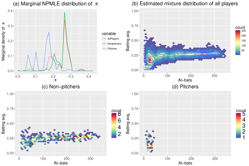
Figure 1: (a) Marginal NPMLE distribution of $\pi$, computed using EM algorithm; (b) histogram of 20,000 independent draws from the estimated distribution of $(A_{j},H_{j}/A_{j})$, fitted with the Poisson-binomial NPMLE to all players in the baseball dataset; (c) histogram of non-pitcher data from the baseball dataset; (d) histogram of pitcher data from the baseball dataset.

8 Two-dimensional NPMLE for cancer microarray classification

Dicker and Zhao (2016) proposed a univariate NPMLE-based method for high-dimensional classification problems and studied applications involving cancer microarray data. The classifiers from Dicker and Zhao (2016) are based on a Gaussian model with one-dimensional mixing distributions, i.e. $d=1$. In this section we show that using a bivariate mixing distribution may substantially improve performance.

Two datasets from the Microarray Quality Control Phase II project (MAQC Consortium, 2010) are considered; one from a breast cancer study and one from a myeloma study. The training dataset for the breast cancer study contains $n=130$ subjects and $p=22283$ probesets (genes); the test dataset contains $100$ subjects. The training dataset for the myeloma study contains $n=340$ subjects and $p=54675$ probesets; the test dataset contains $214$ subjects. The goal is to use the training data to build binary classifiers for several outcomes, then check the performance of these classifiers on the test data. Outcomes for the breast cancer data are response to treatment (“Response”) and estrogen receptor status (“ER status”); outcomes for the myeloma data are overall and event-free survival (“OS” and “EFS”).

For each of the studies, let $X_{ij}$ denote the expression level of gene $j$ in subject $i$ and let $Y_{i}\in\{0,1\}$ be the class label for subject $i$. Let $X_{j}=(X_{1j},\ldots,X_{nj})^{\top}\in{{\mathbb{R}}}^{n}$. We assume that each class ($k=0,1$) and each gene ($j=1,\ldots,p$) has an associated mean expression level $\mu_{jk}\in{{\mathbb{R}}}$, and that conditional on the $Y_{i}$ and $\mu_{jk}$ all of the $X_{ij}$ are independent and Gaussian, satisfying $X_{ij}\mid(Y_{i}=k,\ \mu_{jk})\sim N(\mu_{jk},1)$ (the gene-expression levels in the datasets are all standardized to have variance 1).

In Dicker and Zhao (2016), they assume that $\mu_{1k},\ldots,\mu_{pk}\sim G_{k}$ ($k=0,1$) are all independent draws from two distributions, $G_{0}$ and $G_{1}$. They use the training data from classes $k=0,1$ to separately estimate the distributions $G_{0}$ and $G_{1}$ using NPMLEs, and then implement the Bayes classifier, replacing $G_{0}$ and $G_{1}$ with the corresponding estimates. In this paper, we model $\Theta_{j}=(\mu_{j0},\mu_{j1})\sim G_{0}$ jointly, then compute the bivariate NPMLE $\hat{G}_{\Lambda}$, and finally use $\hat{G}_{\Lambda}$ in place of $G_{0}$ in the Bayes classifier for this model. In the notation of (1), $\Theta_{j}=(\mu_{j0},\mu_{j1})$ and

$$X_{j}\mid\Theta_{j}\sim f_{0}(X_{j}|\Theta_{j})\propto\exp\left[-\frac{1}{2}\sum_{i=1}^{n}\left\{X_{ij}-\sum_{k=0,1}\mu_{jk}\mathbbm{1}(Y_{i}=k)\right\}^{2}\right],$$

where $\mathbbm{1}(\cdot)$ is the indicator function. The model from Dicker and Zhao (2016) is equivalent to the model proposed here, when $\mu_{j0}$ and $\mu_{j1}$ are independent. Results from analyzing the MAQC datasets using these two classifiers (the previously proposed method with 1-dimensional NPMLEs and the 2-dimensional NPMLE described here), along with some other well-known and relevant classifiers, may be found in Table 4. The other classifiers we considered were:

1. NP EBayes w/smoothing. Another nonparametric empirical Bayes classifier proposed in Greenshtein and Park (2009), which uses nonparametric smoothing to fit a univariate density to the $\mu_{jk}$ and then employs a version of linear discriminant analysis.

2. Regularized LDA. A version of $\ell^{1}$-regularized linear discriminant analysis, proposed in Mai et al. (2012).

3. Logistic lasso. $\ell^{1}$-penalized logistic regression fit using the R package glmnet.

Table 4: Microarray data. Number of misclassification errors on test data.

							Logistic
Dataset	Outcome	$n_{\mathrm{test}}$	2d-NPMLE	1d-NPMLE	EBayes	LDA	lasso
Breast	Response	100	15	36	47	30	18
Breast	ER status	100	19	40	39	11	11
Myeloma	OS	214	30	55	100	97	27
Myeloma	EFS	214	34	76	100	63	32

For each of the datasets and outcomes, the 2-dimensional NPMLE classifier substantially outperforms the 1-dimensional NPMLE, and is very competitive with the top performing classifiers. Modeling dependence between $\mu_{j0}$ and $\mu_{j1}$, as with the 2-dimensional NPMLE, seems sensible because most of the genes are likely to have similar expression levels across classes, i.e. $\mu_{j0}$ and $\mu_{j1}$ are likely to be correlated. This may be interpreted as a kind of sparsity assumption on the data, which is prevalent in high-dimensional classification problems. Moreover, our proposed method involving NPMLEs should adapt to non-sparse settings as well, since $G_{0}$ is allowed to be an arbitrary bivariate distribution.

One of the main underlying assumptions of the NPMLE-based classification methods is that the different genes have independent expression levels. This is certainly not true in most applications, but is similar in principle to a “naive Bayes” assumption. Developing methods for NPMLE-based classifiers to better handle correlation in the data may be of interest for future research.

9 Continuous glucose monitoring

The analysis in this section is based on blood glucose data from a study involving 137 type 1 diabetes patients; more details on the study may be found in Hirsch et al. (2008) and Dicker et al. (2013). Subjects in the study were monitored for an average of 6 months each. Throughout the course of the study, each subject wore a continuous glucose monitoring device, built around an electrochemical glucose biosensor. Every 5 minutes while in use, the device records (i) a raw electrical current measurement from the sensor (denoted $\mathrm{ISIG}$), which is known to be correlated with blood glucose density, and (ii) a timestamped estimate of blood glucose density ($\mathrm{CGM}$), which is based on a proprietary algorithm for converting the available data (including the electrical current measurements from the sensor) into blood glucose density estimates. In addition to using the sensors, each study subject maintained a self-monitoring routine, whereby blood glucose density was measured approximately 4 times per day from a small blood sample extracted by fingerstick. Fingerstick measurements of blood glucose density are considered to be more accurate (and are more invasive) than the sensor-based estimates (e.g. CGM). During the study, the result of each fingerstick measurement was manually entered into the continuous monitoring device at the time of measurement; algorithms for deriving continuous sensor-based estimates of blood glucose density, such as $\mathrm{CGM}$, may use the available fingerstick measurements for calibration purposes.

In the rest of this section, we show how NPMLE-based empirical Bayes methods can be used to improve algorithms for estimating blood glucose density using the continuous monitoring data. The basic idea is that after formulating a statistical model relating blood glucose density to $\mathrm{ISIG}$, we allow for the possibility that the model parameters may differ for each subject, then use a training dataset to estimate the distribution of model parameters across subjects (i.e. estimate $G_{0}$) via nonparametric maximum likelihood. This is illustrated for two different statistical models in Sections 9.1–9.2.

Throughout the analysis below, we use fingerstick measurements as a proxy for the actual blood glucose density values. Let $\mathrm{FS}_{j}(t)$ and $\mathrm{ISIG}_{j}(t)$ denote the fingerstick blood glucose density and $\mathrm{ISIG}$ values, respectively, for the $j$-th subject at time $t$. Recall that $\mathrm{FS}_{j}(t)$ is measured, on average, once every 6 hours, while $\mathrm{ISIG}_{j}(t)$ is available every 5 minutes. Let $\mathcal{F}_{t}$ denote the $\sigma$-field of information available at time $t$ (i.e. all of the fingerstick and $\mathrm{ISIG}$ measurements taken before time $t$, plus $\mathrm{ISIG}_{j}(t)$). For each methodology, we use the first half of the available data for each subject to fit a statistical model relating $\mathrm{ISIG}_{j}(t)$ to $\mathrm{FS}_{j}(t)$, then estimate each value $\mathrm{FS}_{j}(t)$ in the second half of the data using $\widehat{\mathrm{FS}}_{j}(t)$, an estimator based on $\mathcal{F}_{t}$. The performance of each method is measured by the MSE on the test data, relative to the MSE of the proprietary estimator $\mathrm{CGM}$.

9.1 Linear model

First we consider a basic linear regression model relating $\mathrm{FS}$ and $\mathrm{ISIG}$,

$$\mathrm{FS}_{j}(t)=\mu_{j}+\beta_{j}\mathrm{ISIG}_{j}(t)+\sigma_{j}\epsilon_{j}(t),\ \ t=t_{1},...,t_{n}$$ (12)

where the $\epsilon_{j}(t)$ are iid $N(0,1)$, $t_{1},...,t_{n}$ is the FS measurement time and $\Theta_{j}=\{\mu_{j},\beta_{j},\log(\sigma_{j})\}\in{{\mathbb{R}}}^{3}$ are unknown, subject-specific parameters. In the notation of (1), $X_{j}=\mathrm{FS}_{j}\equiv\{\mathrm{FS}_{j}(t),t=t_{1},..,t_{n}\}$ and

$$X_{j}\mid\Theta_{j} \sim f_{0}(\mathrm{FS}_{j}|\Theta_{j})$$

$$\propto \exp\left[-n\log\sigma_{j}-\frac{\sum_{i=1}^{n}\big{\{}\mathrm{FS}_{j}(t_{i})-\mu_{j}-\beta_{j}\mathrm{ISIG}_{j}(t_{i})\big{\}}^{2}}{2\exp(2\log\sigma_{j})}\right].$$

Three ways to fit (12) are (i) using the combined model, where $\Theta_{j}=\Theta=\{\mu,\beta,\log(\sigma)\}$ for all $j$, i.e. all the subject-specific parameters are the same; (ii) the individual model, where $\Theta_{1},\ldots,\Theta_{p}$ are all estimated separately, from the corresponding subject data; and (iii) the nonparametric mixture model, where $\Theta_{j}\sim G_{0}$ are iid draws from the $d=3$-dimensional mixing distribution $G_{0}$. For each of these methods, we took $\widehat{\mathrm{FS}}_{j}(t)=\hat{\mu}_{j}+\hat{\beta}_{j}\mathrm{ISIG}(t)$, where $\hat{\mu}_{j}$ and $\hat{\beta}_{j}$ are the corresponding MLEs under the combined and individual models, and, under the mixture model, $\hat{\mu}_{j}={\mathbb{E}}_{\hat{G}_{\Lambda}}(\mu_{j}\mid\mathcal{F}_{t})$ and $\hat{\beta}_{j}={\mathbb{E}}_{\hat{G}_{\Lambda}}(\beta_{j}\mid\mathcal{F}_{t})$. Results are reported in Table 5.

Table 5: Blood glucose data. MSE relative to CGM.

Linear model			Kalman filter
Combined	Individual	NPMLE	Combined	Individual	NPMLE
1.56	1.54	1.51	1.05	1.07	1.03

9.2 Kalman filter

Substantial performance improvements are possible by allowing the model parameters relating $\mathrm{FS}$ and $\mathrm{ISIG}$ to vary with time. In this section we consider the Gaussian state space model (Kalman filter)

$$\begin{array}[]{rcl}\mathrm{FS}_{j}(t_{i})\!\!\!\!&=&\!\!\!\!\alpha_{j}(t_{i})\mathrm{ISIG}_{j}(t_{i})+\sigma_{j}\epsilon_{j}(t_{i-1}),\\ \alpha_{j}(t_{i})\!\!\!\!&=&\!\!\!\!\alpha_{j}(t_{i-1})+\tau_{j}\delta_{j}(t_{i-1}),\end{array}$$ (13)

where we assume that $\mathrm{FS}$ along with $\mathrm{ISIG}$ are observed at times $t_{1},\ldots,t_{n}$ and $\epsilon_{j}(t),\delta_{j}(t)\sim N(0,1)$ are iid. In (13), $\{\alpha_{j}(t)\}$ are the state variables that evolve according to a random walk and $\Theta_{j}=\{\log(\tau_{j}),\log(\sigma_{j})\}$ are unknown parameters. Unlike (12), there is no intercept term in (13); dropping the intercept term has been previously justified when using state space models to analyze glucose sensor data (e.g. Dicker et al., 2013). The parameters $\sigma_{j},\tau_{j}$ control how heavily recent observations are weighted when estimating $\alpha_{j}(t)$.

Similar to the analysis in Section 9.1, we fit (13) using (i) a combined model where $\Theta_{j}=\Theta$ for all $j$; (ii) an individual model where $\Theta_{1},\ldots,\Theta_{p}$ are estimated separately; and (iii) a nonparametric mixture model, where $\Theta_{j}\sim G_{0}$ are iid draws from a $d=2$-dimensional mixing distribution. Under (i)–(ii), $\sigma_{j}$ and $\tau_{j}$ are estimated by maximum likelihood and $\widehat{\mathrm{FS}}_{j}(t_{i})={\mathbb{E}}\{\alpha_{j}(t_{i})\mid\mathcal{F}_{t_{i}}\}\times\mathrm{ISIG}_{j}(t_{i})$, where the conditional expectation is computed with respect to the Gaussian law governed by (13), with $\hat{\sigma}_{j}$ and $\hat{\tau}_{j}$ replacing $\sigma_{j}$ and $\tau_{j}$ (i.e. we use the Kalman filter). For the nonparametric mixture (iii), $\widehat{\mathrm{FS}}_{j}(t_{i})={\mathbb{E}}_{\hat{G}_{\Lambda}}\{\alpha_{j}(t_{i})\mid\mathcal{F}_{t_{i}}\}\times\mathrm{ISIG}_{j}(t_{i})$, where the expectation is computed with respect to the model (13) and the estimated mixing distribution $\hat{G}_{\Lambda}$. Results are reported in Table 5.

9.3 Comments on results

From Table 5, it is evident that the NPMLE mixture approach outperforms the individual and combined methods for both the linear model and the Kalman filter/state space model. The Kalman filter methods perform substantially better than the linear model, highlighting the importance of time-varying parameters (scientifically, this is justified because the sensitivity of the glucose sensor is known to change over time). Note that all of the relative MSE values in Table 5 are greater than 1, indicating that $\mathrm{CGM}$ still outperforms all of the methods considered here. Somewhat more ad hoc methods for estimating blood glucose density that do outperform CGM are described in Dicker et al. (2013); these methods (and CGM) leverage additional data available to the continuous monitoring system, which is not described here for the sake of simplicity. The methods in Dicker et al. (2013) are somewhat similar to the “combined” Kalman filtering method from Section 9.2, where $\Theta_{j}=\Theta$ for all $j$; it would be interesting to see if the performance of these methods could be further improved by using NPMLE ideas.

10 Conclusion

We have proposed a flexible, practical approach to fitting general multivariate mixing distributions with NPMLEs and illustrated the effectiveness of this approach through several real data examples. Theoretically, we proved that the support set of the NPMLE is a subset of the convex hull of MLEs when the likelihood $f_{0}$ comes from a class of elliptical unimodal distributions. We believe that this approach may be attractive for many problems where mixture models and empirical Bayes methods are relevant, offering both effective performance and computational simplicity.

References

-
ApS (2015)
ApS, M., 2015. MOSEK Rmosek Package. Release 8.0.0.46.
URL https://mosek.com/resources/doc/ - Böhning (1995) Böhning, D., 1995. A review of reliable maximum likelihood algorithms for semiparametric mixture models. J. Stat. Plan. Infer. 47, 5–28.
- Böhning et al. (1992) Böhning, D., Schlattmann, P., Lindsay, B. G., 1992. Computer-assisted analysis of mixtures (C.A.MAN): Statistical algorithms. Biometrics 48, 283–303.
- Brown (2008) Brown, L. D., 2008. In-season prediction of batting averages: A field test of empirical Bayes and Bayes methodologies. Ann. Appl. Stat. 2, 113–152.
- DasGupta (2008) DasGupta, A., 2008. Asymptotic Theory of Statistics and Probability. Springer.
- Dicker et al. (2013) Dicker, L. H., Sun, T., Zhang, C.-H., Keenan, D. B., Shepp, L., 2013. Continuous blood glucose monitoring: A Bayes-hidden Markov approach. Stat. Sinica 23, 1595–1627.
- Dicker and Zhao (2016) Dicker, L. H., Zhao, S. D., 2016. High-dimensional classification via nonparametric empirical Bayes and maximum likelihood inference. Biometrika 103, 21–34.
- Donoho and Reeves (2013) Donoho, D. L., Reeves, G., 2013. Achieving Bayes MMSE performance in the sparse signal + Gaussian white noise model when the noise level is unknown. In: IEEE Int. Symp. Inf. Theory. pp. 101–105.
- Efron (2010) Efron, B., 2010. Large-Scale Inference: Empirical Bayes Methods for Estimation, Testing, and Prediction. Cambridge University Press.
- Efron and Morris (1975) Efron, B., Morris, C., 1975. Data analysis using Stein’s estimator and its generalizations. J. Am. Stat. Assoc. 70, 311–319.
- Ferguson (1973) Ferguson, T. S., 1973. A Bayesian analysis of some nonparametric problems. Ann. Stat. 1, 209–230.
- Frank and Wolfe (1956) Frank, M., Wolfe, P., 1956. An algorithm for quadratic programming. Nav. Res. Log. 3, 95–110.
- Ghosal and van der Vaart (2001) Ghosal, S., van der Vaart, A. W., 2001. Entropies and rates of convergence for maximum likelihood and Bayes estimation for mixtures of normal densities. Ann. Stat. 29, 1233–1263.
- Greenshtein and Park (2009) Greenshtein, E., Park, J., 2009. Application of non parametric empirical Bayes estimation to high dimensional classification. J. Mach. Learn. Res. 10, 1687–1704.
- Gu and Koenker (2016) Gu, J., Koenker, R., 2016. On a problem of Robbins. Int. Stat. Rev. 84, 224–244.
- Gu and Koenker (2017a) Gu, J., Koenker, R., 2017a. Empirical Bayesball remixed: Empirical Bayes methods for longitudinal data. J. Appl. Econom. 32 (3), 575–599.
- Gu and Koenker (2017b) Gu, J., Koenker, R., 2017b. Unobserved heterogeneity in income dynamics: An empirical Bayes perspective. J. Bus. Econ. Stat. 35 (1), 1–16.
- Hirsch et al. (2008) Hirsch, I. B., Abelseth, J., Bode, B. W., Fischer, J. S., Kaufman, F. R., Mastrototaro, J., Parkin, C. G., Wolpert, H. A., Buckingham, B. A., 2008. Sensor-augmented insulin pump therapy: Results of the first randomized treat-to-target study. Diabetes Technol. The. 10, 377–383.
- Jaggi (2013) Jaggi, M., 2013. Revisiting Frank-Wolfe: Projection-free sparse convex optimization. ICML 2013 28, 427–435.
- Jiang and Zhang (2009) Jiang, W., Zhang, C.-H., 2009. General maximum likelihood empirical Bayes estimation of normal means. Ann. Stat. 37, 1647–1684.
- Jiang and Zhang (2010) Jiang, W., Zhang, C.-H., 2010. Empirical Bayes in-season prediction of baseball batting averages. In: Borrowing Strength: Theory Powering Applications – A Festschrift for Lawrence D. Brown. Institute of Mathematical Statistics, pp. 263–273.
- Kiefer and Wolfowitz (1956) Kiefer, J., Wolfowitz, J., 1956. Consistency of the maximum likelihood estimator in the presence of infinitely many incidental parameters. Ann. Math. Stat. 27, 887–906.
- Koenker and Gu (2016) Koenker, R., Gu, J., 2016. REBayes: An R package for empirical Bayes mixture methods.