Stabilization of difference equations with noisy proportional feedback control

Abstract.

Given a deterministic difference equation $x_{n+1}=f(x_{n})$, we would like to stabilize any point $x^{\ast}\in(0,f(b))$, where $b$ is a unique maximum point of $f$, by introducing proportional feedback (PF) control. We assume that PF control contains either a multiplicative $x_{n+1}=f\left((\nu+\ell\chi_{n+1})x_{n}\right)$ or an additive noise $x_{n+1}=f(\lambda x_{n})+\ell\chi_{n+1}$. We study conditions under which the solution eventually enters some interval, treated as a stochastic (blurred) equilibrium. In addition, we prove that, for each $\varepsilon>0$, when the noise level $\ell$ is sufficiently small, all solutions eventually belong to the interval $(x^{\ast}-\varepsilon,x^{\ast}+\varepsilon)$.

AMS Subject Classification: 39A50, 37H10, 34F05, 39A30, 93D15, 93C55

Keywords: stochastic difference equations; stabilization; Proportional Feedback control; population models; Beverton-Holt equation

1. Introduction

Difference equations can describe population models with non-overlapping generations. For simplicity, the parameters involved are combined and reduced to a single value in a one-dimensional model. In the logistic equation this parameter describes an intrinsic growth rate. While demonstrating stable dynamics for small parameter values, as the parameter grows, solutions can become chaotic. Thus, even for simplest one-dimensional models, solution behaviour can become complex, resulting in the infinitesimal difference between the two initial values being amplified, leading to unpredictable dynamics. To avoid this situation, either stepwise or periodic types of control were suggested. One of efficient methods of chaos control is the proportional feedback (PF) which consists in the reduction of the state variable at each step (or selected steps), corresponding to harvesting or pest management. For a one-dimensional map

(1.1) $$x_{n+1}=f(x_{n}),\quad x_{0}>0,\quad n\in\mathbb{N},$$

PF method involves reduction of the state variable at each step, proportional to the size of the variable

(1.2) $$x_{n+1}=f(\nu x_{n}),\quad x_{0}>0,\quad n\in\mathbb{N},\quad\nu\in(0,1].$$

This type of control may describe harvesting with a constant effort [12], where the harvest is proportional to the population size, or pest control with constant efficiency [17, 21]. Sometimes reduction boosts population sizes [17, 21], this is called the hydra effect, see, for example, [15] and its literature list. Stabilization with proportional feedback control was recently studied in [6, 11, 14], see also references therein.

Since in many cases there is stochasticity involved in the control, it is reasonable to model population dynamics processes with stochastic equations. Stability of solutions of stochastic difference equations was considered in several publications, see [1, 2, 3, 18, 10, 13, 18] and references therein. Paper [1] proves non-exponential stability and estimates decay rates for solutions of nonlinear equations with unbounded noise, [2] and [13] are focused on local dynamics of polynomial equations with fading stochastic perturbations, in [3] stabilization of difference equations by noise was introduced and justified, [18] is devoted to optimal control for Volterra equations. In [5, 8, 9, 10] stochastic equations connected with population models were considered: [8, 9] discuss stabilization of two-cycles of equations under stochastic perturbations, [10] deals with convergence of solutions of equations with additive perturbations, in [5] stabilization of difference equations with noisy prediction-based control was presented.

Let us assume that the harvesting effort (or management efficiency) varies resulting in a multiplicative noise

(1.3) $$x_{n+1}=f\left((\nu+\ell\chi_{n+1})x_{n}\right),\quad x_{0}>0,\quad n\in\mathbb{N}.$$

It is also possible to suppose that the management efficiency is constant but the environment is stochastic, leading to an additive noise

(1.4) $$x_{n+1}=\max\left\{f(\nu x_{n})+\ell\chi_{n+1},0\right\}.$$

In this paper we impose the assumption on the function $f$ which describes its behaviour in a right neighbourhood of zero.

Assumption 1.1.

The function $f:[0,\infty)\rightarrow[0,\infty)$ is continuous, and there is a real number $b>0$ such that $f(x)$ is strictly monotone increasing, while the function $\frac{f(x)}{x}$ is strictly monotone decreasing on $(0,b]$, $f(b)>b$, while $\frac{f(b)}{b}>\frac{f(x)}{x}$ for any $x\in(b,\infty)$.

Remark 1.2.

Note that, once Assumption 1.1 holds for a certain $b>0$, it is also satisfied for any $b_{1}\in(0,b]$.

For example, the Ricker model

(1.5) $$x_{n+1}=f_{1}(x_{n})=x_{n}e^{r(1-x_{n})}$$

satisfies Assumption 1.1 with $b\leq 1/r$, the truncated logistic model

(1.6) $$x_{n+1}=f_{2}(x_{n})=\max\left\{rx_{n}(1-x_{n}),0\right\}$$

with $r>2$ and $b\leq\frac{1}{2}$. The modifications of the Beverton-Holt equation

$$x_{n+1}=f_{3}(x_{n})=\frac{Ax_{n}}{1+Bx_{n}^{\gamma}},\quad A,B>0,~{}~{}\gamma>1,$$

which is also called a Maynard Smith model [20], and

$$x_{n+1}=f_{4}(x_{n})=\frac{Ax_{n}}{(1+Bx_{n})^{\gamma}},\quad A,B>0,~{}~{}\gamma>1$$

satisfy Assumption 1.1, with the parameters which lead to the existence of a positive equilibrium exceeding the unique maximum point $x_{\max}$ and $b<x_{\max}$. In all the above examples, $f_{i}$ are unimodal: they increase for $x\in[0,x_{\max}]$ and decrease on $[x_{\max},\infty)$, with the only critical point on $[0,\infty)$ being a global maximum.

Note that in Assumption 1.1 we do not assume $f(0)=0$, though in most practical examples, this condition is satisfied. However, $f(0)=0$ does not necessarily imply that a finite limit $\displaystyle\lim_{x\to 0^{+}}\frac{f(x)}{x}$ exists: the Gompertz model with $\displaystyle f(x)=x\ln\left(\frac{K}{x}\right)$ satisfies Assumption 1.1 with $b\leq K/e$, while this limit is $+\infty$. The function $f$ in (1.1) does not need to be unimodal in order to satisfy Assumption 1.1. For example, the equation describing the growth of bobwhite quail populations [16]

(1.7) $$x_{n+1}=x_{n}\left(A+\frac{B}{1+x_{n}^{\gamma}}\right),\quad A,B>0,~{}~{}\gamma>1,$$

in the right-hand side involves a function, which, for some $A$ and $B$, is bimodal, i.e. has two critical points, the smaller of them is a local maximum, while the larger one is a local minimum. However, Assumption 1.1 is satisfied for the function $f(x_{n})$ in the right-hand side of (1.7), with $b$ not exceeding the smallest positive critical point.

In [6], stabilization of any point $x^{\ast}\in(0,b)$ using (1.2) was considered under the following conditions: $f$ increases on $(0,b)$ and satisfies $f(x)>x$, $f^{\prime}(x)>0$ and $f^{\prime\prime}(x)<0$ for $x\in(0,b)$, as well as ${\displaystyle\frac{f(x)}{x}<\frac{f(b)}{b}\,,\quad\forall\;x>b}$.

These conditions imply asymptotic stability [6] and are more restrictive than Assumption 1.1, which, with the appropriate control, also ensures asymptotic stability [4] of an arbitrarily chosen point $x^{\ast}\in(0,b)$, for an appropriate $\nu$. Thus, in the present paper we stick up to less restrictive Assumption 1.1. The condition $f(x)>x$, $x\in(0,b]$ means that all positive fixed points $x$ of the original function $f$ satisfy $x>b$.

However, in the stochastic case, where the noise does not tend to zero as time grows, stabilization in regular sense is impossible: at any stage, a solution will deviate from the equilibrium. We study conditions under which the solution eventually enters some interval, which can be treated as a stochastic (blurred) equilibrium. More exactly, in this paper we stochastically stabilize each point $x^{*}\in(f(0),f(b))$. First, for each $x^{*}\in(f(0),f(b))$ we find $\nu=\nu(x^{*})\in(0,1)$ such that $x^{*}$ becomes a fixed point for the function $g(x):=f(\nu x)$. Afterwards, we determine the maximum noise intensity $\ell$ for which we can guarantee stability of the equilibrium $x^{*}$ in some stochastic sense.

The approach and the results are different in the two cases of equations with multiplicative noise (1.3) and with additive noise (1.4). The main difference is that for the multiplicative noise our results hold almost surely, while for the additive noise we can prove them only with some probability. More exactly, for the solution $x_{n}$ of equation (1.3) with a multiplicative noise and an arbitrary positive initial value $x_{0}$ we show, for each $\varepsilon>0$, that $x_{n}\in(y_{1}-\varepsilon,y_{2}+\varepsilon)$ almost surely, for $n\geq N$, where $N$ is large enough. Here the points $y_{1}$ and $y_{2}$ satisfying $0<y_{1}<y_{2}$ and nonrandom $N$ are defined by the point $x^{*}$, which we are stabilizing, and by the noise intensity $\ell$. We also show that when $\ell\to 0$, the above interval is shrinking to $(x^{*}-\varepsilon,x^{*}+\varepsilon)$. For the solution $x_{n}$ of equation (1.4) with an additive noise and an arbitrary positive initial value $x_{0}$, we show, for each $\varepsilon>0$ and $\gamma\in(0,1)$, the existence of a nonrandom $N=N(\varepsilon,x_{0},\gamma)$ such that probability $\displaystyle\mathbb{P}\{y_{1}\leq x_{n}\leq y_{2}+\varepsilon,\,\,\text{for}\,\,n\geq N\}>\gamma$. In fact, the closer $\gamma$ is to 1, the bigger becomes $N=N(\varepsilon,x_{0},\gamma)$. We also show that when $\ell\to 0$, with probability $\gamma$, the above interval tends to $(x^{*}-\varepsilon,x^{*}+\varepsilon)$.

The paper is organized as follows. In Section 2 we introduce definitions, assumptions and prove some preliminary results. Section 3 considers multiplicative noise. In order to obtain in Section 3.2 the main result for the stochastic equation, we first prove several auxiliary statements for a deterministic equation with variable PF control in Section 3.1. Section 4 deals with additive stochastic perturbations. Similarly to the multiplicative case, first, in Section 4.1 variable deterministic perturbations are studied, and then the main stochastic result is obtained in Section 4.2. Section 5 presents numerical examples illustrating the possibility of stabilization, while Section 6 discusses further developments and new problems arising from the present research.

2. Definitions and preliminaries

Let $(\Omega,{\mathcal{F}},(\mathcal{F}_{n})_{n\in\mathbb{N}},{\mathbb{P}})$ be a complete filtered probability space, $\chi:=(\chi_{n})_{n\in\mathbb{N}}$ be a sequence of independent random variables with the zero mean. The filtration $(\mathcal{F}_{n})_{n\in\mathbb{N}}$ is supposed to be naturally generated by the sequence $(\chi_{n})_{n\in\mathbb{N}}$, i.e. $\mathcal{F}_{n}=\sigma\left\{\chi_{1},\dots,\chi_{n}\right\}$.

In the present paper, we consider (1.3) and (1.4), where the sequence $(\chi_{n})_{n\in{\mathbb{N}}}$ satisfies the following condition.

Assumption 2.1.

$(\chi_{n})_{n\in{\mathbb{N}}}$ is a sequence of independent and identically distributed continuous random variables, with the density function $\phi(x)$ such that

$$\phi(x)>0,\quad x\in[-1,1],\quad\phi(x)\equiv 0,\quad x\notin[-1,1].$$

We use the standard abbreviation “a.s.” for the wordings “almost sure” or “almost surely” with respect to the fixed probability measure $\mathbb{P}$ throughout the text. A detailed discussion of stochastic concepts and notation can be found, for example, in [19].

Now we state some auxiliary results concerning the function $f(\nu x)$, for any $\nu\in(0,1]$. Let Assumption 1.1 hold, then the function $f$ is increasing and continuous when restricted to the interval $(0,b)$. Thus $f$ has the increasing and continuous inverse function

$$f^{-1}:[f(0),f(b)]\to[0,b].$$

Define

(2.1) $$\Phi(z):=\frac{z}{f(z)},\quad z\in(0,b).$$

By Assumption 1.1 the function $\Phi$ is increasing, continuous and therefore uniquely invertible on $(0,b)$. The domain of the inverse function depends on the value of $f(0)$ at zero. Under Assumption 1.1, the limit

$$\lim_{x\to 0^{+}}\frac{f(x)}{x}$$

exists (finite or infinite), is positive and greater than 1. In fact, the function $f(x)/x$ is decreasing on $(0,b)$ and $f(b)/b>1$. Note that if $f(0)>0$ then $\lim_{x\to 0^{+}}\frac{f(x)}{x}=+\infty$, however, in the case $f(0)=0$ the value of the limit can be finite, as well as infinite. Since

$$\frac{f(x)}{x}=\frac{1}{\Phi(x)},$$

we have

$$\lim_{x\to 0^{+}}\frac{f(x)}{x}=\lim_{x\to 0^{+}}\frac{1}{\Phi(x)}.$$

Therefore, we can set

(2.2) $$\Phi(0):=\left\{\begin{array}[]{cc}0,&\text{if}\quad\lim\limits_{x\to 0^{+}}\frac{f(x)}{x}=\infty;\\ \\ \lim\limits_{x\to 0^{+}}\frac{x}{f(x)},&\text{if $\lim\limits_{x\to 0^{+}}\frac{f(x)}{x}\in(1,\infty)$ }.\end{array}\right.$$

Thus, we have proved the following lemma.

Lemma 2.2.

Let Assumption 1.1 hold, and $\Phi$ be defined as in (2.1) and (2.2). Then

1. $\Phi:(0,b)\to\left(\Phi(0),\Phi(b)\right),\quad\Phi^{-1}:\biggl{(}\Phi(0),\Phi(b)\biggr{)}\to(0,b)$;
   

2. $0\leq\Phi(0)<\Phi(b)<1$;
   

3. both functions, $\Phi$ and $\Phi^{-1}$, are increasing and continuous on their domains specified in (i).

For each point $x^{*}\in(f(0),f(b))$, we are looking for the control parameter $\nu=\nu(x^{*})\in(0,1)$ such that $x^{*}$ is the fixed point of the function $g(x):=f(\nu x)$. Define

(2.3) $$\nu=\nu(x^{*}):=\Phi(f^{-1}(x^{*})).$$

Lemma 2.3.

Let Assumption 1.1 hold. For each $x^{*}\in(f(0),f(b))$, the control $\nu(x^{*})$ defined by (2.3), satisfies the following conditions:

1. $x^{*}$ is a fixed point of the function $g(x):=f(\nu x)$, i.e. $f\bigl{(}\nu(x^{*})x^{*}\bigr{)}=x^{*}$;

2. $\nu(x^{*})\in\left(\Phi(0),\,\Phi(b)\right)\subset(0,1)$;

3. $\nu(x^{*})$ is an increasing function of $x^{*}$ on $(f(0),f(b))$.

Proof.

For each $x^{*}\in(f(0),f(b))$, we have

$$\nu(x^{*})=\Phi(f^{-1}(x^{*}))=\frac{f^{-1}(x^{*})}{f(f^{-1}(x^{*}))}=\frac{f^{-1}(x^{*})}{x^{*}},$$

so

$$f\bigl{(}\nu(x^{*})x^{*}\bigr{)}=f\left(\frac{f^{-1}(x^{*})}{x^{*}}x^{*}\right)=f\left(f^{-1}(x^{*})\right)=x^{*},$$

which implies (i).

Since $x^{*}\in(f(0),f(b))$,

$$f^{-1}(x^{*})\in(0,b),$$

and by Lemma 2.2 we have

$$\nu(x^{*})\in\left(\Phi(0),\,\Phi(b)\right)\subset(0,1),$$

which proves (ii). Since both $\Phi$ and $f^{-1}$ are increasing functions on $(0,b)$ and $(f(0),f(b))$, respectively, we conclude that $\nu(x^{*})=\Phi(f^{-1}(x^{*}))$ is increasing as a function of $x^{*}$ on $(f(0),f(b))$, which concludes the proof of (iii). ∎

Finally, let us discuss the role of the inequality $f(b)>b$ in Assumption 1.1. If we omit this condition in Assumption 1.1, we should also consider $b$ such that $f(b)\leq b$. Using the assumptions that $f(b)\leq b$ and the function $\Phi(x)=\frac{x}{f(x)}$ is continuous and monotone increasing on $(0,b]$, we get that $\Phi(x)<1$ for small $x>0$ and $\Phi(b)\geq 1$. Thus there is the only point $x^{\ast}\in(0,b]$ where $\Phi(x^{\ast})=1$, or $f(x^{\ast})=x^{\ast}$. According to Assumption 1.1, the continuous function $f$ is monotone increasing on $[0,x^{\ast}]$, $f(x)\geq x$ for $x\in[0,x^{\ast}]$ and $f(x)<x$ for $x>x^{\ast}$. By [6, Lemma 1], see also [4], these conditions guarantee that all solutions of equation (1.1) with $x_{0}>0$ tend to $x^{\ast}$ as $n\to\infty$. Thus, under $f(b)\leq b$ the unique positive equilibrium $x^{\ast}$ is stable, and there is no need to apply any control to stabilize $x^{\ast}$. This is the reason why we consider only the case when $f(b)>b$.

3. Multiplicative Perturbations

In this section we consider the deterministic PF with variable intensity $\nu_{n}\in(0,1]$

(3.1) $$x_{n+1}=f\left(\nu_{n}x_{n}\right),\quad x_{0}>0,\quad n\in\mathbb{N},$$

and then corresponding stochastic equation (1.3) with a multiplicative noise. For each $x^{*}\in\bigl{(}f(0),f(b)\bigr{)}$, we establish the control $\nu=\nu(x^{*})$ and the interval such that a solution of (1.3) remains in this interval, once the level of noise $\ell$ is small enough.

3.1. Deterministic multiplicative perturbations

In Lemma 3.1 below we prove that when intensity $\nu_{n}$ belongs to some interval, solution $x_{n}$ of (3.1) will reach and remain in another interval for big enough $n$.

As discussed in Section 2, Assumption 1.1 implies that for any $\displaystyle\mu\in\left(\Phi(0),\,\Phi(b)\right)$ there is a $y=\Phi^{-1}(\mu)\in(0,b)$, where $\Phi$ is defined in (2.1) and (2.2).

Lemma 3.1.

Let Assumption 1.1 hold, and $\mu_{1}$, $\mu_{2}$ be such that

(3.2) $$\mu_{1}\in\left(\Phi(0),\Phi(b)\right),\quad\mu_{2}\in\left(\Phi(0),\mu_{1}\right),$$

and, for each $n\in{\mathbb{N}}$,

(3.3) $$\nu_{n}\in[\mu_{2},\mu_{1}].$$

Then, for any $x_{0}>0$ and $\varepsilon>0$, there is $n_{0}\in{\mathbb{N}}$ such that the solution $x_{n}$ of equation (3.1) for any $n\geq n_{0}$ satisfies

$$\nu_{n}x_{n}\in\left(\Phi^{-1}(\mu_{2})-\varepsilon,\Phi^{-1}(\mu_{1})+\varepsilon\right).$$

Proof.

Define

$$y_{1}:=\Phi^{-1}(\mu_{1}),\quad y_{2}:=\Phi^{-1}(\mu_{2}).$$

Lemma 2.2 implies that, as $\Phi(0)<\mu_{2}<\mu_{1}<\Phi(b)$, we have

$$0<y_{2}<y_{1}<b.$$

By (3.2) and (3.3), for each $n\in\mathbb{N}$,

(3.4) $$\Phi(0)<\Phi(y_{2})\leq\nu_{n}\leq\Phi(y_{1})<\Phi(b).$$

The proof consists of three main steps. First, we prove that for any $x_{0}>0$ there is an $n_{1}\in{\mathbb{N}}$ such that $\nu_{n}x_{n}\in(0,b)$ for $n\geq n_{1}$. Next, we show that for any $\varepsilon\in\left(0,b-y_{1}\right)$, there is an $n_{2}(\varepsilon)\in{\mathbb{N}}$, $n_{2}(\varepsilon)>n_{1}$, such that $\nu_{n}x_{n}\in(0,y_{1}+\varepsilon)$, $n\geq n_{2}(\varepsilon)$. And, finally, we verify that for any $\varepsilon\in\left(0,y_{1}\right)$, there is an $n_{3}\in{\mathbb{N}}$, $n_{3}>n_{2}(\varepsilon)$, such that $\nu_{n}x_{n}\in(y_{2}-\varepsilon,y_{1}+\varepsilon)$, $n\geq n_{3}$.

First, assume that $\nu_{n}x_{n}\geq b$ for some $n\in{\mathbb{N}}$. Then, (3.2), (3.3) and Assumption 1.1 imply $f(\nu_{n}x_{n})/(\nu_{n}x_{n})\leq f(b)/b$ and

$$\nu_{n+1}x_{n+1} = \nu_{n+1}f\left(\nu_{n}x_{n}\right)=\nu_{n+1}\nu_{n}x_{n}\frac{f\left(\nu_{n}x_{n}\right)}{\nu_{n}x_{n}}$$

$$\leq \nu_{n+1}\nu_{n}x_{n}\frac{f(b)}{b}\leq\mu_{1}\frac{f(b)}{b}\nu_{n}x_{n}=\lambda\nu_{n}x_{n},$$

where

$$\lambda:=\mu_{1}\,\frac{f(b)}{b}\in(0,1).$$

We obtained that the positive sequence $\nu_{j}x_{j}$, $j\geq n$ does not exceed a geometric sequence: $\nu_{j}x_{j}\leq\lambda^{j-n}\nu_{n}x_{n}$ with $\lambda\in(0,1)$, as long as $\nu_{j-1}x_{j-1}\geq b$. If $\nu_{k}x_{k}>b$ for the subsequent $k=n,n+1,\dots$, we get $\nu_{j}x_{j}<b$ for $j>n+[(\ln b-\ln(\nu_{n}x_{n}))/\ln\lambda]+1$, where $[t]$ is the integer part of $t$. Thus for some $n_{1}\in{\mathbb{N}}$, $x_{n_{1}}$ satisfies $\nu_{n_{1}}x_{n_{1}}<b$.

Further, to verify that $\nu_{j}x_{j}<b$ for any $j\geq n_{1}$, we note that, by (3.4), $\displaystyle\frac{\Phi(y_{1})}{\Phi(b)}=\frac{y_{1}}{f(y_{1})}\frac{f(b)}{b}<1$ and also $\nu_{j+1}\leq\mu_{1}$. Then, if $\nu_{j}x_{j}<b$, we have

$$\nu_{j+1}x_{j+1} = \nu_{j+1}f\left(\nu_{j}x_{j}\right)\leq\mu_{1}f\left(\nu_{j}x_{j}\right)$$

$$= \frac{y_{1}}{f(y_{1})}f\left(\nu_{j}x_{j}\right)<\frac{y_{1}}{f(y_{1})}f(b)=\frac{y_{1}}{f(y_{1})}\,\frac{f(b)}{b}\,b<b.$$

Thus, once $\nu_{n_{1}}x_{n_{1}}<b$, all $\nu_{j}x_{j}<b$, $j\geq n_{1}$.

Second, assuming $\nu_{n}x_{n}\in(y_{1},b)$, we have by (3.4)

$$\nu_{n+1}x_{n+1}=\nu_{n+1}\nu_{n}x_{n}\frac{f\left(\nu_{n}x_{n}\right)}{\nu_{n}x_{n}}\leq\nu_{n+1}\nu_{n}x_{n}\frac{f(y_{1})}{y_{1}}<\frac{y_{1}}{f(y_{1})}\nu_{n}x_{n}\frac{f(y_{1})}{y_{1}}=\nu_{n}x_{n}.$$

Thus, once some $\nu_{n}x_{n}\in(y_{1},b)$, we have $\nu_{n+1}x_{n+1}<\nu_{n}x_{n}<b$ as well.

Next, let us take some $\varepsilon\in(0,b-y_{1})$. In the previous computation we apply $y_{1}+\varepsilon$ instead of $y_{1}$. Then, once $\nu_{n}x_{n}\geq y_{1}+\varepsilon$, we have $x_{n+1}\leq\lambda^{\ast}x_{n}$, with

$$\lambda^{\ast}:=\frac{f(y_{1}+\varepsilon)}{y_{1}+\varepsilon}\,\frac{y_{1}}{f(y_{1})}=\mu_{1}\,\frac{f(y_{1}+\varepsilon)}{y_{1}+\varepsilon}\in(0,1)\,.$$

If $\nu_{k}x_{k}\geq y_{1}+\varepsilon$ for the subsequent $k=n,n+1,\dots$ then $\nu_{j}x_{j}<y_{1}+\varepsilon$ for $j>n+[(\ln(y_{1}+\varepsilon)-\ln(\nu_{n}x_{n}))/\ln(\lambda^{\ast})]+1$. Thus $\nu_{n}x_{n}<y_{1}+\varepsilon$ for any $\varepsilon>0$ and $n\geq n_{2}(\varepsilon)\in{\mathbb{N}}$, for some $n_{2}(\varepsilon)>n_{1}$.

Let us justify, that, if $\nu_{n}x_{n}\leq y_{1}+\varepsilon<b$, all the subsequent $x_{k}$ also satisfy this inequality. If $\nu_{n}x_{n}\leq y_{1}+\varepsilon<b$ then, by monotonicity of $f$ on $[0,y_{1}+\varepsilon]$ and since now $\mu_{1}=\Phi(y_{1})<\Phi(y_{1}+\varepsilon)$, we have

$$\nu_{n+1}x_{n+1}=\nu_{n+1}f(\nu_{n}x_{n})\leq\nu_{n+1}f(y_{1}+\varepsilon)<\frac{\nu_{n+1}(y_{1}+\varepsilon)}{\mu_{1}}\leq y_{1}+\varepsilon,$$

as $\nu_{n+1}\leq\mu_{1}$.

Finally, for any $\varepsilon\in(0,y_{2})$, if $\nu_{n}x_{n}<y_{2}-\varepsilon$, we obtain

$$\nu_{n+1}x_{n+1}=\nu_{n+1}\nu_{n}x_{n}\frac{f\left(\nu_{n}x_{n}\right)}{\nu_{n}x_{n}}\geq\nu_{n+1}\nu_{n}x_{n}\frac{f(y_{2}-\varepsilon)}{y_{2}-\varepsilon}\geq\mu_{2}\nu_{n}x_{n}\frac{f(y_{2}-\varepsilon)}{y_{2}-\varepsilon}=\lambda_{1}\nu_{n}x_{n},$$

where

$$\lambda_{1}:=\mu_{2}\frac{f(y_{2}-\varepsilon)}{y_{2}-\varepsilon}\in(1,\infty).$$

Thus, $\nu_{n+1}x_{n+1}\geq\lambda_{1}\nu_{n}x_{n}$ as long as $\nu_{n}x_{n}<y_{2}-\varepsilon$. Hence, as in the second part of the proof, there is $N_{2}(\varepsilon)\in{\mathbb{N}}$ such that $\nu_{n}x_{n}>y_{2}-\varepsilon$ for $n\geq N_{2}(\varepsilon)$. If $\nu_{n}x_{n}\in(y_{2}-\varepsilon,b]$ then, as $f$ is monotone on $[0,b]$ and by (3.4),

$$\nu_{n+1}x_{n+1}=\nu_{n+1}f(\nu_{n}x_{n})\geq\mu_{2}\frac{f(y_{2}-\varepsilon)}{y_{2}-\varepsilon}\,(y_{2}-\varepsilon)>\mu_{2}\frac{y_{2}-\varepsilon}{\mu_{2}}=y_{2}-\varepsilon.$$

Thus, for any $x_{0}>0$ and $\varepsilon>0$, for $n\geq n_{3}>\max\{N_{2}(\varepsilon),n_{2}(\varepsilon)\}$ we have $\nu_{n}x_{n}\in(y_{2}-\varepsilon,y_{1}+\varepsilon)$, which concludes the proof. ∎

Remark 3.2.

In Lemma 3.1 we actually proved that, for small   $\varepsilon>0$,   once $\nu_{n}x_{n}\in(y_{1}-\varepsilon,y_{2}+\varepsilon)$, all subsequent $\nu_{n+j}x_{n+j}$, $j\in{\mathbb{N}}$, are also in this interval. This is also true for the results based on Lemma 3.1, in particular, for Lemma 3.3 and Theorem 3.4.

3.2. Stochastic multiplicative perturbations.

Now   we   proceed   to   stochastic   equation (1.3). First, we prove a lemma which can be treated as a stochastic version of Lemma 3.1 and can be easily deduced from it.

Lemma 3.3.

Suppose that Assumptions 1.1 and 2.1 hold, $\Phi$ is defined as in (2.1), $x^{*}\in(f(0),f(b))$, $\nu=\nu(x^{*})$ is defined as in (2.3), and $\ell\in\mathbb{R}$ satisfies the inequality

(3.5) $$0<\ell<\min\left\{\Phi(b)-\nu,\,\,\nu-\Phi(0)\right\}.$$

Let $x_{n}$ be a solution to equation (1.3) with $\nu$ satisfying (2.3), $\ell$ satisfying (3.5) and an arbitrary initial value $x_{0}>0$. Then, for any $\varepsilon>0$ there is $N_{0}\in{\mathbb{N}}$ such that, for all $n\geq N_{0}$,

$$\left(\nu+\ell\chi_{n+1}\right)x_{n}\in\left(\Phi^{-1}(\nu-\ell)-\varepsilon,\Phi^{-1}(\nu+\ell)+\varepsilon\right),\mbox{~{}~{}a.s.}$$

Proof.

From Lemma 2.3 we conclude that

$$\nu(x^{*})=\Phi(f^{-1}(x^{*}))\in\left(\Phi(0),\,\Phi(b)\right).$$

So the right-hand side of (3.5) is positive. With $\nu$ defined in (2.3) and $\ell$ satisfying (3.5), we have, a.s.,

$$\nu_{n}=\nu+\ell\chi_{n+1}\leq\nu+\ell$$

and

$$\nu_{n}=\nu+\ell\chi_{n+1}\geq\nu-\ell,$$

so $\nu_{n}=\nu+\ell\chi_{n+1}\in(\nu-\ell,\nu+\ell)$, a.s.

Now we let $\mu_{1}:=\nu-\ell$, $\mu_{2}:=\nu+\ell$ and apply Lemma 3.1. ∎

Lemma 3.3 implies the main result of this section, which states that for each $x^{*}\in(0,f(b))$ we can find a control $\nu$ and a noise level $\ell$, such that the solution eventually reaches and stays in some interval, defined by $\nu$ and $\ell$, a.s.

Theorem 3.4.

Let Assumptions 2.1, 1.1 hold, $\Phi$ be defined as in (2.1), $x^{*}\in(f(0),f(b))$ be an arbitrary point, $\nu=\nu(x^{*})$ be defined as in (2.3), $x_{0}>0$ and $\ell\in\mathbb{R}$ satisfy inequality (3.5). Then for the solution $x_{n}$ of equation (1.3), the following statements are valid, a.s.

1. For each $\delta>0$ there exists a nonrandom $N=N(\delta)\in\mathbb{N}$ such that, for all $n\geq N$,

   $$x_{n}\in\left(\frac{\Phi^{-1}(\nu-\ell)}{\nu+\ell}-\delta,\,\,\frac{\Phi^{-1}(\nu+\ell)}{\nu-\ell}+\delta\right).$$

2. $\displaystyle\liminf_{n\to\infty}x_{n}\geq\frac{\Phi^{-1}(\nu-\ell)}{\nu+\ell},\quad\limsup_{n\to\infty}x_{n}\leq\frac{\Phi^{-1}(\nu+\ell)}{\nu-\ell}.$

Proof.

Note that condition (3.5) implies $\nu>\ell$. Fix $\delta>0$ and take some $\varepsilon>0$ satisfying

$$\varepsilon<\delta(\nu-\ell).$$

By Lemma 3.3, for any $x_{0}>0$ and $\varepsilon>0$, there is $N_{0}=N_{0}(\varepsilon)\in\mathbb{N}$ such that, a.s.,

$$(\nu+\ell\chi_{n+1})x_{n}>\Phi^{-1}(\nu-\ell)-\varepsilon,\quad(\nu+\ell\chi_{n+1})x_{n}<\Phi^{-1}(\nu+\ell)+\varepsilon,\quad n\geq N_{0}.$$

Since $x_{n}\geq 0$ and $\nu+\ell\chi_{n+1}\in(\nu-l,\nu+l)$ we have, a.s.,

$$\Phi^{-1}(\nu-\ell)-\varepsilon<(\nu+\ell\chi_{n+1})x_{n}\leq(\nu+\ell)x_{n}$$

and

$$\Phi^{-1}(\nu+\ell)+\varepsilon>(\nu+\ell\chi_{n+1})x_{n}\geq(\nu-\ell)x_{n}.$$

Therefore, for $n\geq N_{0}$ we get, a.s.,

(3.6) $$\frac{\Phi^{-1}(\nu-\ell)-\varepsilon}{\nu+\ell}<x_{n}<\frac{\Phi^{-1}(\nu+\ell)+\varepsilon}{\nu-\ell}.$$

Since

$$\frac{\varepsilon}{v+\ell}<\delta,\quad\frac{\varepsilon}{v-\ell}<\delta,$$

from inequality (3.6) we obtain (i).

As $\delta>0$ in (i) is arbitrary, (i) immediately implies (ii). ∎

Theorem 3.5 below deals with the situation when the noise level $\ell$ can be chosen arbitrarily small. It confirms the intuitive feeling that, as the noise level $\ell$ is getting smaller, the solution of stochastic equation (1.2) behaves similarly to the solution of correspondent deterministic equation (1.2) in terms of approaching its stable equilibrium $x^{*}$.

Theorem 3.5.

Let Assumptions 1.1 and 2.1 hold, $x^{*}\in(f(0),f(b))$ be an arbitrary point, $\nu=\nu(x^{*})$ be defined as in (2.3), and $x_{0}>0$ be an arbitrary initial value. Then for any $\varepsilon>0$, there exists the level of noise $\ell(\varepsilon)>0$ such that for each $\ell<\ell(\varepsilon)$, there is a positive integer $N_{1}=N_{1}(\varepsilon,\ell,x_{0})$ such that for the solution $x_{n}$ of the equation (1.3) with $n\geq N_{1}$ we have $x_{n}\in(x^{*}-\varepsilon,x^{*}+\varepsilon)$, a.s.

Proof.

For each $\delta>0$, $x^{*}\in(f(0),f(b))$, $\nu(x^{*})=\Phi(f^{-1}(x^{*}))$ and $\ell$ satisfying (3.5), the solution $x_{n}$ of equation (1.3) with an arbitrary initial value $x_{0}>0$ satisfies inequality (3.6) for $n\geq N_{0}=N_{0}(\delta,\ell,x_{0})$, which can be written as

$$\frac{\Phi^{-1}(\Phi(f^{-1}(x^{*}))-\ell)-\delta}{\nu+l}<x_{n}<\frac{\Phi^{-1}(\Phi(f^{-1}(x^{*}))+\ell)+\delta}{\nu-l}.$$

By continuity of $\Phi$ we have

$$\lim_{\ell\to 0}\frac{\Phi^{-1}(\Phi(f^{-1}(x^{*}))-\ell)}{\Phi(f^{-1}(x^{*}))+\ell}=\frac{\Phi^{-1}(\Phi(f^{-1}(x^{*})))}{\Phi(f^{-1}(x^{*}))}=\frac{f^{-1}(x^{*})}{\frac{f^{-1}(x^{*})}{x^{*}}}=x^{*}$$

and

$$\lim_{\ell\to 0}\frac{\Phi^{-1}(\Phi(f^{-1}(x^{*}))+\ell)}{\Phi(f^{-1}(x^{*}))-\ell}=\frac{\Phi^{-1}(\Phi(f^{-1}(x^{*})))}{\Phi(f^{-1}(x^{*}))}=\frac{f^{-1}(x^{*})}{\frac{f^{-1}(x^{*})}{x^{*}}}=x^{*}.$$

Then, for each $\delta>0$, we obtain

(3.7) $$\lim_{\ell\to 0}\frac{\Phi^{-1}(\Phi(f^{-1}(x^{*}))-\ell)-\delta}{\Phi(f^{-1}(x^{*}))+\ell}=\frac{f^{-1}(x^{*})-\delta}{\frac{f^{-1}(x^{*})}{x^{*}}}=x^{*}-\delta\frac{x^{*}}{f^{-1}(x^{*})}$$

and

(3.8) $$\lim_{\ell\to 0}\frac{\Phi^{-1}(\Phi(f^{-1}(x^{*}))+\ell)+\delta}{\Phi(f^{-1}(x^{*}))-\ell}=\frac{f^{-1}(x^{*})+\delta}{\frac{f^{-1}(x^{*})}{x^{*}}}=x^{*}+\delta\frac{x^{*}}{f^{-1}(x^{*})}.$$

Fix some $\varepsilon>0$ as in the statement of the theorem and take

(3.9) $$\delta=\frac{\varepsilon}{2}\,\,\frac{f^{-1}(x^{*})}{x^{*}}.$$

Applying (3.7) and (3.8), for $\delta$ defined by (3.9) we can find $\ell(\varepsilon)>0$ such that, for $\ell<\ell(\varepsilon)$, both inequalities below hold:

(3.10) $$\begin{split}&\frac{\Phi^{-1}(\Phi(f^{-1}(x^{*}))-\ell)-\delta}{\Phi(f^{-1}(x^{*}))+\ell}>x^{*}-\delta\frac{x^{*}}{f^{-1}(x^{*})}-\frac{\varepsilon}{2}=x^{*}-\varepsilon,\\ &\frac{\Phi^{-1}(\Phi(f^{-1}(x^{*}))+\ell)+\delta}{\Phi(f^{-1}(x^{*}))-\ell}<x^{*}+\delta\frac{x^{*}}{f^{-1}(x^{*})}+\frac{\varepsilon}{2}=x^{*}+\varepsilon.\end{split}$$

Fix some $\ell<\ell(\varepsilon)$ and find, for $\ell$ and $\delta$ (defined by (3.9)), a number $N_{1}=N_{1}(\varepsilon,\ell,x_{0})$ such that, for all $n\geq N_{1}$,

(3.11) $$\frac{\Phi^{-1}(\Phi(f^{-1}(x^{*}))-\ell)-\delta}{\Phi(f^{-1}(x^{*}))+\ell}<x_{n}<\frac{\Phi^{-1}(\Phi(f^{-1}(x^{*}))+\ell)+\delta}{\Phi(f^{-1}(x^{*}))-\ell}.$$

By applying inequalities (3.10) to inequality (3.11) we arrive at

$$x^{*}-\varepsilon<x_{n}<x^{*}+\varepsilon,\quad n\geq N_{1},$$

which concludes the proof. ∎

4. Additive Perturbations

In this section we investigate similar problems for the stochastic equation with additive perturbations, i.e. equation (1.4), where $f$ satisfies Assumption 1.1.

Our purpose remains the same: to pseudo-stabilize any point $x^{*}\in\bigl{(}f(0),f(b)\bigr{)}$. For each $x^{*}\in\bigl{(}f(0),f(b)\bigr{)}$, we establish the control $\nu=\nu(x^{*})$ and the interval such that a solution remains in this interval, once the noise level $\ell$ is small enough. For any $x^{*}\in\bigl{(}f(0),f(b)\bigr{)}$, the same $\nu=\Phi(f^{-1}(x^{*}))$ as in the previous section will work.

4.1. Deterministic additive perturbations

Before   considering   stochastic difference equation (1.4) with an additive noise, we first study a deterministic model with variable perturbations

(4.1) $$x_{n+1}=\max\left\{f\left(\nu x_{n}\right)+r_{n},0\right\},\quad r_{n}\in{\mathbb{R}},\quad x_{0}>0,\quad n\in\mathbb{N},$$

as well as its version without a proportional feedback

(4.2) $$x_{n+1}=\max\left\{g(x_{n})+r_{n},0\right\},\quad r_{n}\in{\mathbb{R}}\quad x_{0}>0,\quad n\in\mathbb{N}.$$

The function $g$ can also be viewed as a function in which a control has already been incorporated, for example, $g(x)=f(\nu x)$.

Assumption 4.1.

Assume that the function $g:[0,\infty)\rightarrow[0,\infty)$ is continuous, and there is a real number $c>0$ such that $g(x)$ is strictly monotone increasing, while the function $\frac{g(x)}{x}$ is strictly monotone decreasing on $(0,c]$, $\frac{g(c)}{c}>\frac{g(x)}{x}$ for any $x>c$, and there exists a unique fixed point $x^{*}\in(0,c)$ of $g$ on $(0,\infty)$, $g(x^{\ast})=x^{*}$.

Remark 4.2.

Note that Assumption 4.1 and Assumption 1.1 are the same except the conditions: $f(b)>b$ while $g(c)<c.$

Let $d>0$ satisfy

(4.3) $$d<\min\left\{c-g(c),\max_{x\in[0,x^{\ast}]}\left[g(x)-x\right]\right\}.$$

Introduce the numbers $y_{1}$, $y_{2}$ and $y_{3}$ as follows:

(4.4) $$\begin{split}y_{1}:=&\sup\left\{\left.x\in[0,x^{\ast}]\right|g(x)-x\geq d\right\}\in(0,x^{\ast}),\\ y_{2}:=&\inf\left\{\left.x\in[x^{\ast},c]\right|g(x)-x\leq-d\right\}\in(x^{\ast},c),\end{split}$$

and

(4.5) $$y_{3}=\inf\left\{\left.x\in[x^{\ast},\infty)\right|g(x)-d\leq y_{1}\right\},$$

where we assume $y_{3}=\infty$, if the set in the right-hand-side of (4.5) is empty; see Fig. 1 for the outline of the points $y_{i}$, $i=1,2,3$.

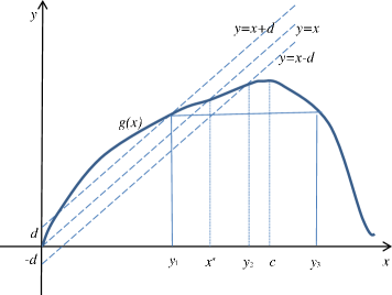
Figure 1. The graph of $g(x)$ with $y_{i}$, $i=1,2,3$, together with the equilibrium $x^{\ast}$ marked

Lemma 4.3.

Suppose Assumption 4.1 holds and $d$ satisfies (4.3). Then

1. the numbers $y_{1}$, $y_{2}$ and $y_{3}$ defined by (4.4) and (4.5), respectively, exist;

2. $y_{1}$ and $y_{2}$ satisfy

   (4.6) $$0<y_{1}<x^{\ast}<y_{2}<c,\quad g(y_{1})-d=y_{1},\quad g(y_{2})+d=y_{2},$$

   $y_{2}\in(x^{*},c)$ is the only solution of $g(x)+d=x$ on $[x^{\ast},\infty)$, and $g(x)+d<x$ for $x>y_{2}$;

3. either finite or infinite $y_{3}$ satisfies $y_{3}>c$ and $g(x)-d\geq y_{1}$ for $x\in[y_{1},y_{3}]$, if $y_{3}<\infty$, and for $x\in[y_{1},\infty)$ if $y_{3}=\infty$.

Proof.

Note that $g(0)\geq 0$, $g({x}^{*})=x^{*}$, $g(x)-x$ is continuous and, due to (4.3), we have $\max_{x\in[0,x^{\ast}]}\left[g(x)-x\right]=g(x_{\max})-x_{\max}>d$ for some $x_{\max}\in[0,x^{\ast})$. Thus, $g(x^{*})-x^{*}<d$ and there is $x\in(0,x^{\ast})$ such that $g(x)-x>d$, which implies $y_{1}\in(0,x^{\ast})$.

Further, the equations $g(x)=x-d$ and $g(x)=x+d$ have solutions on $(0,c]$. By (4.3), $g(c)+d<c$, while $g(x^{\ast})+d=x^{\ast}+d>x^{\ast}$. As $g(x)+d$ is continuous, there is a point $y_{2}\in(x^{\ast},c)$ such that $g(y_{2})+d=y_{2}$. Moreover, $\displaystyle\frac{g(x)+d}{x}$ is a decreasing function on $[x^{\ast},c]$, and for $x>c$, it is less than $(g(c)+d)/c<1$, since

$$\frac{g(x)+d}{x} = \frac{g(x)}{x}+\frac{d}{x}<\frac{g(c)}{c}+\frac{d}{c}$$

$$\leq \frac{g(y_{2})}{y_{2}}+\frac{d}{y_{2}}=\frac{g(y_{2})+d}{y_{2}}=1.$$

Thus, there is exactly one fixed point of $g(x)+d$ on $[x^{\ast},\infty)$, where the function $\displaystyle\frac{g(x)+d}{x}$ equals one, which is $y_{2}$, and $g(x)+d<x$ for $x>x^{\ast}$.

By (4.4), we have $y_{1}\in(0,x^{\ast})$ and $g(y_{1})-d=y_{1}$. Since $g$ increases and is continuous on $[0,c]$, and so is $g(x)-d$, we have $g(x)-d>y_{1}$ for any $x\in(y_{1},c]$, therefore $y_{3}>c$. Relations (4.4) and (4.5) imply $g(x)-d\geq y_{1}$ for $x\in[y_{1},y_{3}]$, if $y_{3}<\infty$, and for $x\in[y_{1},\infty)$ if $y_{3}=\infty$. ∎

Lemma 4.4.

Suppose that Assumption 4.1 holds, $d$ satisfies (4.3), and $y_{1}$, $y_{2}$, $y_{3}$ are defined by (4.4) and (4.5), respectively.

Let $x_{n}$ be a solution of (4.2) with $-d\leq r_{n}\leq d$ and $x_{0}\in[y_{1},y_{3}]$. Then

1. for each $\varepsilon>0$ there exists $N=N(\varepsilon,x_{0})$ such that, for $n\geq N$,

   (4.7) $$y_{1}\leq x_{n}\leq y_{2}+\varepsilon;$$

2. we have

   (4.8) $$\liminf_{n\to\infty}x_{n}\geq y_{1},\quad\limsup_{n\to\infty}x_{n}\leq y_{2}.$$

Proof.

By Lemma 4.3, (iii), if $x_{0}\in[y_{1},y_{3}]$ then

$$x_{1}=g(x_{0})+r_{0}\geq g(x_{0})-d\geq y_{1},$$

so $x_{1}\geq y_{1}$. By (4.3), for $x\leq c$,

$$g(x)+d<g(c)+c-g(c)=c.$$

By Lemma 4.3, (ii), for $x_{0}\geq x^{\ast}$

$$g(x_{0})+d\leq x_{0}.$$

Thus, $x_{0}\leq y_{3}$ implies

$$x_{1}\leq g(x_{0})+|r_{0}|\leq g(x_{0})+d\leq\max\{x_{0},c\}\leq y_{3}.$$

Similarly, $x_{n}\in[y_{1},y_{3}]$ yields that $x_{n+1}\in[y_{1},y_{3}]$; consequently, the first equalities in (4.7) and (4.8) hold.

For each $x_{n}\leq y_{2}$, by monotonicity of $g$ on $[0,c]$ and by (4.4),

$$x_{n+1}\leq g(x_{n})+|r_{n}|\leq g(y_{2})+d=y_{2}.$$

By Lemma 4.3, (ii), if $x_{n}\in(y_{2},y_{3}]$ then $g(x_{n})+d<x_{n}$, and thus

$$x_{n+1}\leq g(x_{n})+|r_{n}|\leq g(x_{n})+d<x_{n}.$$

Assuming that all $x_{n}\in(y_{2},y_{3}]$, we obtain that it is a decreasing sequence which has a limit $s\geq y_{2}$. Thus $x_{n}<x_{1}$, and $s>y_{2}$ implies

$$x_{n}-x_{n+1}\geq x_{n}-g(x_{n})-d\geq\min_{x\in[s,x_{1}]}\left[x-g(x)-d\right]=\sigma>0.$$

Then $\lim_{n\to\infty}x_{n}=-\infty$, which contradicts to $x_{n}\geq s>y_{2}$.

Hence for any $x_{0}\in(y_{2},y_{3}]$ and $\varepsilon>0$, we need a finite number of steps $N=N(\varepsilon,x_{0})$ to reach $(y_{1},y_{2}+\varepsilon)$, which proves the right inequality in (4.7).

Thus $\limsup_{n\to\infty}x_{n}\leq y_{2}$, and the second equality in (4.8) is also satisfied, which concludes the proof. ∎

Lemma 4.5.

Let Assumption 1.1 hold, $x^{*}\in(f(0),f(b))$ be an arbitrary point, and $\nu=\nu(x^{*})$ be defined as in (2.3). Suppose that

(4.9) $$g(x):=f(\nu x),\quad c:=\frac{b}{\nu}\,,$$

$d$ satisfies (4.3), and $y_{1}$, $y_{2}$, $y_{3}$ are defined in (4.4) and (4.5), respectively.

Then all solutions of (4.1) with $-d\leq r_{n}\leq d$ and $x_{0}\in[y_{1},y_{3}]$ satisfy parts (i) and (ii) of Lemma 4.4.

Proof.

Once we show that $g$ satisfies Assumption 4.1, the result will follow from Lemma 4.4.

From (2.1) and (2.3) we have

$$\nu=\Phi\left(f^{-1}(x^{\ast})\right)=\frac{f^{-1}(x^{\ast})}{x^{\ast}}\in(0,1),$$

and, by Lemma 2.3, (i), $g$ has $x^{*}$ as a fixed point. Also, $g$ is continuous and increasing on $\displaystyle\left[0,c\right]$. For $x>c$, we have $\nu x>b$, and thus

$$\frac{g(x)}{x}=\frac{f\left(\nu x\right)}{x}=\nu\,\frac{f\left(\nu x\right)}{\nu x}<\nu\,\frac{f(b)}{b}=\frac{g\left(c\right)}{c}.$$

Note that

$$\frac{g\left(c\right)}{c}=\nu\,\frac{f(b)}{b}=\frac{f^{-1}(x^{\ast})}{x^{\ast}}\,\frac{f(b)}{b}=\frac{\Phi\left(f^{-1}(x^{\ast})\right)}{\Phi(b)}$$

and $g(x)/x$ is strictly monotone decreasing on $(0,c]$, since for $0<x_{1}<x_{2}\leq c$ we have

$$\frac{g(x_{1})}{x_{1}}=\nu\frac{f(\nu x_{1})}{\nu x_{1}}>\nu\frac{f(\nu x_{2})}{\nu x_{2}}=\frac{g(x_{2})}{x_{2}}$$

by Assumption 1.1, so $\displaystyle\frac{g(x)}{x}<\frac{g(c)}{c}$ for $x>c$. Since $f^{-1}(x^{\ast})<b$ and $\Phi$ is strictly increasing, we have

$$\frac{\Phi\left(f^{-1}(x^{\ast})\right)}{\Phi(b)}<1,\quad\text{therefore}\quad\frac{g\left(c\right)}{c}<1.$$

Thus $g(x)<x$ for $x\geq c$, and $g$ cannot have a fixed point on $(c,\infty)$. Assume that there is one more fixed point $y$ of $g$ on $(0,c)$ and $y\neq x^{\ast}$. Since $y\in(0,c)$, we have $\nu y\in(0,b)$ and

$$g(y)=f\left(\nu y\right)=y,\quad\text{or}\quad f\left(\frac{f^{-1}(x^{\ast})}{x^{\ast}}y\right)=y.$$

Then the fixed point $y$ should be in $(0,f(b))$, and thus $f^{-1}(y)$ is well defined. Therefore

$$\frac{f^{-1}(x^{\ast})}{x^{\ast}}y=f^{-1}(y),$$

which implies

$$\Phi\left(f^{-1}(x^{\ast})\right)=\frac{f^{-1}(x^{\ast})}{x^{\ast}}=\frac{f^{-1}(y)}{y}=\Phi\left(f^{-1}(y)\right).$$

However, $\Phi\left(f^{-1}(y)\right)$ is strictly increasing on $(f(0),f(b))$, hence $y=x^{\ast}$. Application of Lemma 4.4 concludes the proof. ∎

4.2. Stochastic additive noise

In this section, we consider stochastic difference equation (1.4). First we state a lemma which will be used in the proof of the main result and which was proved in [5].

Lemma 4.6.

[5] Let $\xi_{1},\dots,\xi_{n},\dots$ be a sequence of independent identically distributed random variables such that $\mathbb{P}\left\{\xi\in(a,b)\right\}=\tau\in(0,1)$ for some interval $(a,b)$, $a<b$. Let $\mathcal{N}_{0}$ be an a.s. finite random number. Then for each $J\in{\mathbb{N}_{0}}$,

$$\mathbb{P}\biggl{[}\text{\rm{There exists} }\mathcal{N}^{*}=\mathcal{N}^{*}(J)\in(\mathcal{N}_{0},\infty)\\ \text{ \rm{such that} }\xi_{\mathcal{N}^{*}}\in(a,b),\,\xi_{\mathcal{N}^{*}+1}\in(a,b),\dots,\xi_{\mathcal{N}^{*}+J}\in(a,b)\biggr{]}=1.$$

The next theorem is the main result of this section which states that, for each $\varepsilon>0$, there exists a number after which a solution of equation (1.4) will reach the interval $[y_{1},y_{2}+\varepsilon]$ and stay there forever. However, in contrast to Theorem 3.4, where such a number is nonrandom and applies to all solutions a.s., Theorem 4.7 only proves, for each $\omega\in\Omega$, the existence of its own $\mathcal{N}(\omega)$ such that $x_{\mathcal{N}(\omega)}\in[y_{1},y_{2}+\varepsilon]$ . In addition, it is shown that, with an arbitrarily close to 1 probability, there is a nonrandom $N$ such that $x_{n}\in[y_{1},y_{2}+\varepsilon]$ for $n\geq N$.

Theorem 4.7.

Let Assumptions 1.1 and 2.1 hold, $x^{*}\in(f(0),f(b))$ be an arbitrary point, and $\nu=\nu(x^{*})$ be chosen as in (2.3), $g$ and $c$ be defined as in (4.9), and $d$ satisfy (4.3). Suppose that $y_{1}$, $y_{2}$, $y_{3}$ are defined as in (4.4) and (4.5), respectively, and $x_{n}$ is a solution to equation (1.4) with an arbitrary $x_{0}>0$ and $\ell>0$ satisfying

(4.10) $$\ell\leq d.$$

Then

1. for each $\varepsilon>0$, there exists a random $\mathcal{N}(\omega)=\mathcal{N}(\omega,x_{0},\ell,x^{*},\varepsilon)$ such that for $n\geq\mathcal{N}(\omega)$ we have, a.s. on $\Omega$,

   (4.11) $$y_{1}\leq x_{n}\leq y_{2}+\varepsilon;$$

2. for each $\varepsilon>0$ and each $\gamma\in(0,1)$, there exists a nonrandom $N=N(\gamma,x_{0},\ell,x^{*},\varepsilon)$ such that

   (4.12) $$\mathbb{P}\{y_{1}\leq x_{n}\leq y_{2}+\varepsilon,\,\,\text{\rm{for}}\,\,n\geq N\}>\gamma;$$

3. we have

   (4.13) $$\liminf_{n\to\infty}x_{n}\geq y_{1},\quad\limsup_{n\to\infty}x_{n}\leq y_{2},\quad\text{a.s}.$$

Proof.

(i) In view of Lemma 4.5, we have to prove first that for the solution $x_{n}$ of (1.4) with an arbitrary initial value $x_{0}>0$, there exists a random a.s. finite $\mathcal{N}_{1}(\omega)=\mathcal{N}_{1}(\omega,x_{0},\ell,x^{*})$ such that for $n\geq\mathcal{N}_{1}(\omega)$ we have $x_{n}\in[y_{1},y_{3}]$, a.s. on $\Omega$.

The proof consists of two parts. First, we verify that for $x_{0}>y_{3}$ there exists a nonnrandom $K\in\mathbb{N}$ such that $x_{n}\leq y_{3}$ for $n\geq K$; this part certainly is worth considering only for $y_{3}<\infty$. We also show that $x_{k}<y_{1}$ implies $x_{k+1}<y_{3}$. Second, we find a random a.s. finite $\mathcal{N}_{1}=\mathcal{N}_{1}(\omega,x_{0},\ell,x^{*})$ such that $x_{\mathcal{N}_{1}}(\omega)\in[y_{1},y_{3}]$ and a random $\mathcal{N}(\omega)=\mathcal{N}(\omega,x_{0},\ell,x^{*},\varepsilon)$ such that (4.11) holds for $n\geq\mathcal{N}(\omega)$.

Assume that $y_{3}<\infty$ and recall that $y_{3}>c>y_{2}$, see Lemma 4.3, (ii), and Fig. 1.

Let $x_{k}\in(y_{3},\infty)$ for some $k\in\mathbb{N}$. Since $d<c-g(c)$ by (4.3) and $g(x)/x<g(c)/c$ for $x>c$,

$$\frac{g(x_{k})+\ell\chi_{1}}{x_{k}}\leq\frac{g(x_{k})}{x_{k}}+\frac{\ell}{x_{k}}<\frac{g(c)+d}{c}<\frac{c-d+d}{c}=1,$$

so the next sequence term is smaller: $x_{k+1}<x_{k}$. Moreover, denoting

$$\lambda:=\frac{g(c)+\ell}{c}<1,$$

we have $x_{k+1}\leq\lambda x_{k}$, as long as $x_{k}\in(y_{3},\infty)$. Thus, whenever $x_{0}>y_{3}$, after at most $K$ steps, where

(4.14) $$K>\ln\left.\left(\frac{y_{3}}{x_{0}}\right)\right/\ln\lambda\,,$$

we have $x_{K}\in[0,y_{3}]$.

If $x_{k}<y_{1}$, condition (4.3), $0<c<y_{3}$ and the fact that $g$ is monotone increasing on $[0,c]$ imply

$$x_{k+1}\leq g(x_{k})+d<g(c)+c-g(c)=c<y_{3}.$$

Thus, $x_{k+1}<y_{3}$ for any $x_{k}<y_{1}$. So we conclude that for each $x_{0}>0$ and $K$ defined as in (4.14), the solution reaches the interval $[0,y_{3}]$ after at most $K$ steps.

Now we proceed to the second part of the proof, assuming that $x_{0}<y_{1}$. By Assumption 2.1, for any $\varepsilon_{0}\in(0,1)$, the probability $p_{1}$ of the following event is positive:

$$p_{1}:={\mathbb{P}}\left\{\chi\in[\varepsilon_{0},1]\right\}>0.$$

By (4.6) we have $y_{1}<x^{\ast}$, therefore $x_{k}\in[0,y_{1})$ implies $g(x_{k})>x_{k}$. If in addition $\chi_{k+1}\in[\varepsilon_{0},1]$, we have

$$x_{k+1}=g(x_{k})+\ell\chi_{k+1}>x_{k}+\ell\varepsilon_{0}.$$

Fix $\varepsilon_{0}\in(0,1)$ and define

$$J:=\left[\frac{y_{1}}{\ell\varepsilon_{0}}\right]+1.$$

If $J$ successive $\chi_{j}$, starting with $\chi_{k+1}$, satisfy $\chi_{j}\in[\varepsilon_{0},1]$, we have either $x_{k+j}\geq y_{1}$, for some $j=1,2,\dots,J-1$, or

$$x_{k+J}>x_{k}+J\ell\varepsilon_{0}>y_{1}.$$

By Lemma 4.6, a.s., there is a sequence of such $J$ successive $\chi_{j}$, which starts from an a.s. finite random number $\mathcal{N}^{*}$.

Summarizing all of the above, we conclude that for $x_{0}>y_{3}$ after $n\leq K$ steps we have $x_{n}\in[0,y_{3}]$. If $x_{n}<y_{1}$ we need at most $\mathcal{N}^{*}+J$ steps to reach $[y_{1},y_{3}]$. Once $x_{n}\in[y_{1},y_{3}]$, all $x_{n+k}\in[y_{1},y_{3}]$, $k\in\mathbb{N}$. Thus, by Lemma 4.6, for

(4.15) $$n\geq\mathcal{N}_{1}=K+\mathcal{N}^{*}+J$$

we have $x_{n}\in[y_{1},y_{3}]$, a.s.

Fix some $\varepsilon>0$. Suppose that $x_{n}\in[y_{2}+\varepsilon,y_{3}]$, where $n$ satisfies (4.15), and apply Lemmata 4.4-4.5, considering $x_{n}=x_{n(\omega)}$ as the initial value for each $\omega\in\Omega$. Then, for each $\omega\in\Omega$, Lemmata 4.4-4.5 claim the existence of an a.s. finite number $\mathcal{N}_{2}(x_{n(\omega)},\varepsilon)$ such that the solution will be in $[y_{1},y_{2}+\varepsilon]$ after $\mathcal{N}_{2}$ steps. Denoting

$$\mathcal{N}=\mathcal{N}(x_{0},\varepsilon,\ell,x^{*}):=K+\mathcal{N}^{*}+J+\mathcal{N}_{2},$$

we conclude that

(4.16) $$x_{n}\in[y_{1},y_{2}+\varepsilon]\quad\text{for any $n\geq\mathcal{N}$},$$

which completes the proof of (i).

Since $\mathcal{N}(x_{0},\varepsilon,\ell,x^{*})$ is a.s. finite, we can define

$$\Omega_{i}:=\{\omega\in\Omega:i-1\leq\mathcal{N}<i\}.$$

Note that $\Omega=\bigcup_{i=1}^{\infty}\Omega_{i}$ and $\Omega_{i}\bigcap\Omega_{j}=\emptyset$ for all $i\neq j$, therefore $\sum\limits_{i=1}^{\infty}\mathbb{P}(\Omega_{i})=1$.

For any $\gamma\in(0,1)$, we define $\Omega(\gamma):=\bigcup_{i=1}^{N}\Omega_{i}$, where $N=N(\gamma,x_{0},\ell,x^{*},\varepsilon)\in\mathbf{N}$ is such that

$$\sum_{i=1}^{N}\mathbb{P}(\Omega_{i})\in(\gamma,1).$$

Then,

$$\mathcal{N}(x_{0},\varepsilon,\ell,x^{*})\leq N(\gamma,x_{0},\ell,x^{*},\varepsilon)\quad\text{on}\quad\Omega(\gamma),\quad\text{and}\quad\mathbb{P}(\Omega_{\gamma})>\gamma.$$

This completes the proof of (ii). Part (iii) follows from (4.16) since $\varepsilon>0$ is arbitrary. ∎

The next theorem deals with the situation when the level of noise can be decreased. It shows that a solution will eventually be in any arbitrarily small neighborhood of the point $x^{\ast}$ with arbitrarily close to 1 probability.

Theorem 4.8.

Let Assumptions 1.1 and 2.1 hold, $x_{0}>0$ be an arbitrary initial value, $x^{*}\in(f(0),f(b))$ be an arbitrary point, $\nu=\nu(x^{*})$ be chosen as in (2.3).

Then, for each $\varepsilon>0$ and $\gamma\in(0,1)$, we can find $d$ such that for the solution $x_{n}$ to (1.4) with $\ell\leq d$, and for some nonrandom $N=N(\gamma,x_{0},\ell,x^{*},\varepsilon)\in\mathbb{N}$, we have

$$\mathbb{P}\{x_{n}\in(x^{*}-\varepsilon,x^{*}+\varepsilon)\,\,\text{for all $n\geq N$}\}\geq\gamma.$$

Proof.

Let $g$ and $c$ be defined as in (4.9) and let $x_{\max}$ be a point (maybe not unique) where the function $g(x)-x$ attains its maximum on $[0,x^{*}]$:

$$g(x_{\max})-x_{\max}=\max_{x\in[0,x^{*}]}\{g(x)-x\}.$$

Note that, for each $d$ satisfying (4.3), the values $y_{1}$ and $y_{2}$ defined by (4.4) satisfy

$$y_{1}\in(x_{\max},x^{*}),\quad y_{2}\in(x^{*},c),$$

and $y_{1}=y_{1}(d)$, $y_{2}=y_{2}(d)$. Let us show that

$$\lim_{d\to 0}y_{1}(d)=\lim_{d\to 0}y_{1}(d)=x^{*}.$$

To this end, define

$$\Psi(x)=\frac{g(x)}{x},\quad x>0.$$

By Assumption 4.1, the function $\Psi$ decreases and is continuous on $(0,c)$, so it has an inverse function $\Psi^{-1}$, which also decreases and is continuous on $(\Psi(0),\Psi(c))$. We have $\Psi(x^{*})=1$ and

$$g(y_{1})-y_{1}=d,\quad y_{2}-g(y_{2})=d.$$

So, by dividing each of the above equations by $y_{1}$ and $y_{2}$, respectively, we arrive at

$$\frac{g(y_{1})}{y_{1}}-1=\frac{d}{y_{1}},\quad 1-\frac{g(y_{2})}{y_{2}}=\frac{d}{y_{2}}.$$

This leads to the estimates

$$1<\Psi(y_{1})=1+\frac{d}{y_{1}}<1+\frac{d}{x_{\max}}\to 1\quad\text{as}\quad d\to 0$$

and

$$1>\Psi(y_{2})=1-\frac{d}{y_{2}}>1-\frac{d}{x^{*}}\to 1\quad\text{as}\quad d\to 0.$$

Hence

(4.17) $$\begin{split}x^{*}=&\Psi^{-1}(1)>y_{1}(d)>\Psi^{-1}\left(1+\frac{d}{x_{\max}}\right)\to x^{*}\quad\text{as}\quad d\to 0,\\ x^{*}=&\Psi^{-1}(1)<y_{2}(d)<\Psi^{-1}\left(1-\frac{d}{x^{*}}\right)\to x^{*}\quad\text{as}\quad d\to 0.\end{split}$$

Now, fix some $\varepsilon>0$ and find $\delta$ such that

(4.18) $$\left|\Psi^{-1}\left(1+u\right)-\Psi^{-1}\left(1\right)\right|<\frac{\varepsilon}{2}\quad\text{as soon as}\quad|u|<\delta.$$

Let $d$, in addition to (4.3), satisfy

$$d<\delta x^{*}.$$

Then, from (4.17) and (4.18), we obtain that

(4.19) $$\begin{split}y_{1}(d)>&\Psi^{-1}(1)+\left[\Psi^{-1}\left(1+\frac{d}{x_{\max}}\right)-\Psi^{-1}(1)\right]\geq x^{*}-\frac{\varepsilon}{2},\\ y_{2}(d)<&\Psi^{-1}(1)+\left[\Psi^{-1}\left(1+\frac{d}{x^{*}}\right)-\Psi^{-1}(1)\right]\geq x^{*}+\frac{\varepsilon}{2}.\end{split}$$

Further, we work only with $\ell\leq d$. Applying part (ii) of Theorem 4.7 for $\varepsilon/2$ and $\gamma\in(0,1)$, we find a nonrandom $N=N(\gamma,x_{0},\ell,x^{*},\varepsilon)\in\mathbb{N}$ and $\Omega_{\gamma}\subset\Omega$ with $\mathbb{P}(\Omega_{\gamma})>\gamma$, such that for each $\omega\in\Omega_{\gamma}$ and $n\geq N$ we have

$$y_{1}\leq x_{n}\leq y_{2}+\frac{\varepsilon}{2}.$$

This, along with inequalities (4.19), gives us the desired result: for each $n\geq N$, we have on  $\Omega_{\gamma}$

$$x^{*}-\frac{\varepsilon}{2}<y_{1}\leq x_{n}\leq y_{2}+\frac{\varepsilon}{2}<x^{*}+\varepsilon,$$

which concludes the proof. ∎

5. Numerical Examples

In this section, we consider two examples: the Beverton-Holt chaotic map

(5.1) $$f(x)=\frac{2.5x}{1+x^{5}},\quad x\geq 0,$$

considered in [6] and a particular case of (1.7)

(5.2) $$f(x)=x\left(0.55+\frac{3.45}{1+x^{9}}\right),\quad x\geq 0,$$

introduced in [16] and also considered in [7].

Example 5.1.

We can show that the function $f$ defined in (5.1) is increasing, up to its maximum attained at $b=2^{-2/5}\approx 0.757858$. Also,

$$f(b)=f(2^{-2/5})=2\times 2^{-2/5}\approx 1.5157,$$

and

$$\Phi(0)=\lim_{x\to 0}\frac{x}{f(x)}=\lim_{x\to 0}\frac{1+x^{5}}{2.5}=0.4,\quad\Phi(b)=\frac{b}{f(b)}=\frac{1+2^{-2}}{2.5}=0.5.$$

Based on the results of Sections 3 and 4 we conclude that with PF control we can stabilize any point $x^{*}\in(f(0),f(b))=(0,2b)\approx(0,1.5157)$ with corresponding $\nu$-values belonging to the interval $(\Phi(0),\Phi(b))=(0,0.5)$.

For example, we can stabilize $x^{*}=1.5$, which can be achieved for $\nu\approx 0.4685$. In Fig. 2, we get a blurry equilibrium centered at $x^{*}=1.5$ with smaller $\ell=0.01$ (upper left) and larger $\ell=0.025$ (upper right). In the other graphs $\ell=0.015$ and five runs for each parameter set are presented, where we stabilize $x^{*}=1.125$ ($\nu\approx 0.415033$) and $x^{*}=1.1$ ($\nu\approx 0.40721$) in the medium row and present the two cases where all solutions tend to zero ($\nu=0.39<0.4$, lower left) or are not stabilized ($\nu=0.75>0.5$, lower right) in the lower row.

Figure 2. Solutions of the difference equation with $f$ as in (5.1) and multiplicative stochastic perturbations with $\ell=0.01$ (upper left), $\ell=0.025$ (upper right), where PF control aims at stabilizing $x^{*}=1.5$, $\nu\approx 0.4685$ and $\ell=0.015$ (two lower rows), with either $x^{*}=1.125$ (second row,left) or $x^{*}=1.1$ stabilized (second row, right), and $x^{*}=0$ is stabilized for $\nu=0.39$ (lower left); for $\nu=0.75$ there is no blurred equilibrium but oscillations (lower right). Everywhere $x_{0}=0.5$.

In Fig. 3 the same runs are presented for the case of the additive noise.

Figure 3. Solutions of the difference equation with $f$ as in (5.1) and additive stochastic perturbations with $\ell=0.01$ (upper left), $\ell=0.025$ (upper right), where PF control aims at stabilizing $x^{*}=1.5$, $\nu\approx 0.4685$ and $\ell=0.015$ (two lower rows), with either $x^{*}=1.125$ (second row,left) or $x^{*}=1.1$ stabilized (second row, right), and $x^{*}=0$ is stabilized for $\nu=0.39$ (lower left); for $\nu=0.75$ there is no blurred equilibrium but oscillations (lower right). Everywhere $x_{0}=0.5$.

Example 5.2.

Let us apply PF control to (5.2). We can stabilize $x^{*}=2.5$, which can be achieved for $\nu\approx 0.253555$. The dependency of the solution variation on $\ell$ is illustrated in Fig. 4, for $\ell=0.01$ (left) and $\ell=0.025$ (right). In Fig. 5, left, we stabilize the maximum $\approx 2.877$ of the function in the right-hand side of (5.2), with $\nu\approx 0.282$, in the middle, with $\nu=0.23$, the zero equilibrium is stabilized, while the right figure corresponds to the blurred cycle with $\nu=0.35$.

Figure 4. Solutions of the difference equation with $f$ as in (5.2) and multiplicative stochastic perturbations with $\ell=0.01$ (left) and $\ell=0.025$ (right), where PF control aims at stabilizing $x^{*}=2.5$, $\nu\approx 0.253555$. In both figures, five runs are illustrated, $x_{0}=1$.

Figure 5. Solutions of the difference equation with $f$ as in (5.2) and multiplicative stochastic perturbations with $\ell=0.01$, where we stabilize the maximum $\approx 2.877$ (left), the zero equilibrium with $\nu=0.23$ (middle) and obtained blurred cycle for $\nu=0.35$ (right). Everywhere we present five runs, $x_{0}=1$.

In Fig. 6 we ullustrate stabilization of $x^{*}=2.5$ with $\nu\approx 0.253555$ and additive noise with $\ell=0.01$ (left) and oscillation with $\nu=0.35$ (right).

Figure 6. Solutions of the difference equation with $f$ as in (5.2) and additive stochastic perturbations with $\ell=0.01$, where $x^{*}=2.5$ is stabilized (left), or there are sustainable blurred oscillations for $\nu=0.35$ (right). In each figure, we present five runs, $x_{0}=1$.

6. Discussion and Open Problems

In the present paper we considered PF stabilization, and the approach is a little bit different than in [6, 11, 14] where an appropriate range of stabilizing $\nu$ was established, and the stabilization point was found for any of such $\nu$. Here we focus on the range of points that can be stabilized with PF control, and, once such $x^{*}$ is chosen, we identify the required control level. In addition, either the control or the environment can be stochastic, we get a stable blurred equilibrium as a result of the control. Numerical examples illustrate that

1. the stochasticity in the control can lead to higher solution variation than the stochasticity of the environment (compare Figs. 2 and 3);

2. there is a strong dependency of this variation on both the form of the function $f$ involved in the difference equation and the point to be stabilized (compare the right top and the middle figures in Fig. 2).

Though we deal with stochastic perturbations with a constant maximal amplitude, statements for this amplitude tending to zero give an indication that results for a stochastic perturbation tending to zero with time will be similar to the non-stochastic PF control [11, 14]. Certainly stochasticity of the control and the environment can be combined.

Some relevant open problems and topics for future research are outlined below.

1. Estimate the probability of certain solution bounds if the conditions of the theorems of the present paper are not satisfied, for example, in the case of the Allee effect.

2. Consider unbounded, for example, normally distributed, perturbations.

3. Explore the equation with both multiplicative and additive noise

   $$x_{n+1}=f\left((\nu+l_{1}\chi_{n+1})x_{n}\right)+l_{2}\zeta_{n+1},\,\,x_{0}>0,\quad n\in\mathbb{N},$$

   describing a model where both the harvesting effort (or pest management efficiency) and the environment are stochastic.

4. Investigate the case where not a positive equilibrium but a cycle can be stabilized, with a control applied at each step.

5. Consider the equation where a stochastic control is applied on certain steps only, so called “impulsive” control [6] and consider stabilization of blurred cycles.

References

- [1] J. A. D. Appleby, G. Berkolaiko, and A. Rodkina. Non-exponential stability and decay rates in nonlinear stochastic difference equations with unbounded noise. Stochastics: An International Journal of Probability and Stochastic Processes, 81:2, (2009), 99-127.
- [2] J. A. D. Appleby, C. Kelly, X. Mao, and A. Rodkina, On the local dynamics of polynomial difference equations with fading stochastic perturbations. Dynamics of Continuous, Discrete and Impulsive Systems. A. 17 (3), (2010), 401-430.
- [3] J. A. D. Appleby, X. Mao, and A. Rodkina. On stochastic stabilization of difference equations, Dynamics of Continuous and Discrete System, 15:3, (2006), pp. 843-857.
- [4] E. Braverman and B. Chan, Stabilization of prescribed values and periodic orbits with regular and pulse target oriented control, Chaos 24 (2014), article 013119, 7p.
- [5] E. Braverman, C. Kelly, A. Rodkina, Stabilisation of difference equations with noisy prediction-based control, to appear in Physica D, 2016, DOI: 10.1016/j.physd.2016.02.004.
- [6] E. Braverman and E. Liz, Global stabilization of periodic orbits using a proportional feedback control with pulses, Nonlinear Dynamics 67 (2012), 2467–2475.
- [7] E. Braverman and E. Liz, On stabilization of equilibria using predictive control with and without pulses, Comput. Math. Appl. 64 (2012), 2192–2201.
- [8] E. Braverman, A. Rodkina, Stabilization of two-cycles of difference equations with stochastic perturbations, J. Difference Equ. Appl. 19 (2013), 1192–1212.
- [9] E. Braverman, A. Rodkina, Difference equations of Ricker and logistic types under bounded stochastic perturbations with positive mean, Comput. Math. Appl. 66 (2013), 2281–2294.
- [10] E. Braverman and A. Rodkina, On convergence of solutions to difference equations with additive perturbations, to appear in J. Difference Equ. Appl. (2016), http://dx.doi.org/10.1080/10236198.2016.1161762.
- [11] P. Carmona and D. Franco, Control of chaotic behaviour and prevention of extinction using constant proportional feedback, Nonlinear Anal. Real World Appl. 12 (2011), 3719–3726.
- [12] C. W. Clark, Mathematical bioeconomics: the optimal management of renewable resources, 2nd Edition, John Wiley & Sons, Hoboken, New Jersey, 1990.
- [13] C. Kelly and A. Rodkina, Constrained stability and instability of polynomial difference equations with state-dependent noise, Discrete Contin. Dyn. Syst. 11 (2009),
- [14] E. Liz, How to control chaotic behaviour and population size with proportional feedback, Phys. Lett. A 374 (2010), 725–728.
- [15] E. Liz and A. Ruiz-Herrera, The hydra effect, bubbles, and chaos in a simple discrete population model with constant effort harvesting, J. Math. Biol. 65 (2012), 997–-1016.
- [16] J.G. Milton and J. Bélair, Chaos, noise, and extincion in models of population growth, Theor. Popul. Biol. 37 (1990), 273–290.
- [17] H. Seno, A paradox in discrete single species population dynamics with harvesting/thinning, Math. Biosci. 214 (2008), 63–69.
- [18] L. Shaikhet, Optimal Control of Stochastic Difference Volterra Equations. An Introduction. Studies in Systems, Decision and Control 17, Springer, Cham, 2015.
- [19] A. N. Shiryaev (1996): Probability (2nd edition), Springer, Berlin.
- [20] H.R. Thieme, Mathematics in Population Biology, Princeton University Press, Princeton, 2003.
- [21] E. F. Zipkin, C. E. Kraft, E. G. Cooch, and P. J. Sullivan, When can efforts to control nuisance and invasive species backfire?, Ecological Applications 19 (2009), 1585-1595.