BICEP2 / Keck Array VIII: Measurement of gravitational lensing from large-scale $B$-mode polarization

Abstract

We present measurements of polarization lensing using the 150 GHz maps which include all data taken by the BICEP2 & Keck Array CMB polarization experiments up to and including the 2014 observing season (BK14). Despite their modest angular resolution ($\sim 0.5^{\circ}$), the excellent sensitivity ($\sim 3\mu$K-arcmin) of these maps makes it possible to directly reconstruct the lensing potential using only information at larger angular scales ($\ell\leq 700$). From the auto-spectrum of the reconstructed potential we measure an amplitude of the spectrum to be $A_{\rm L}^{\phi\phi}=1.15\pm 0.36$ (Planck $\Lambda$CDM prediction corresponds to $A_{\rm L}^{\phi\phi}=1$), and reject the no-lensing hypothesis at $5.8\sigma$, which is the highest significance achieved to date using an $EB$ lensing estimator. Taking the cross-spectrum of the reconstructed potential with the Planck 2015 lensing map yields $A_{\rm L}^{\phi\phi}=1.13\pm 0.20$. These direct measurements of $A_{\rm L}^{\phi\phi}$ are consistent with the $\Lambda$CDM cosmology, and with that derived from the previously reported BK14 $B$-mode auto-spectrum ($A_{\rm L}^{\rm BB}=1.20\pm 0.17$). We perform a series of null tests and consistency checks to show that these results are robust against systematics and are insensitive to analysis choices. These results unambiguously demonstrate that the $B$-modes previously reported by BICEP / Keck at intermediate angular scales ($150\lesssim\ell\lesssim 350$) are dominated by gravitational lensing. The good agreement between the lensing amplitudes obtained from the lensing reconstruction and $B$-mode spectrum starts to place constraints on any alternative cosmological sources of $B$-modes at these angular scales.

I. Introduction

Cosmic Microwave Background (CMB) photons traveling from the surface of last scattering are lensed by the gravitational potential of the large-scale structure along the line of sight. This leads to spatial distortions of a few arcminutes in the temperature and polarization anisotropies. In particular, gravitational lensing converts some of the $E$-mode polarization into $B$-mode polarization (Zaldarriaga & Seljak, 1998). Measurements of temperature and polarization with sufficient resolution and sensitivity can be used to reconstruct the intervening matter distribution, and in the future such bias-free measurements of large-scale structure will become some of the most powerful probes in cosmology (e.g., Hu 2002; Namikawa et al. 2010; Wu et al. 2014; Abazajian et al. 2015; Allison et al. 2015; Pan & Knox 2015). Lensing can also act as a noise source for primordial $B$-modes, which peak at degree-scales (e.g., Kesden et al. 2002; Knox & Song 2002). With sufficient sensitivity, a reconstructed lensing potential can be used to predict the degree-scale lensing $B$-modes, enabling a deeper search for a primordial signal. If the tensor-to-scalar ratio $r$ is below $0.01$, such “de-lensing” procedures will become important in the search for inflationary $B$-modes (Kesden et al., 2002; Knox & Song, 2002; Seljak & Hirata, 2004; Smith et al., 2012). In the latest BICEP / Keck results we already see a non-negligible lensing contribution at large angular scales ($\ell<100$) (Bicep2 / Keck Array Collaboration VI, 2015).

Lensing reconstruction from high resolution CMB temperature maps has been performed using data from the Atacama Cosmology Telescope (ACT; Das et al. 2011, 2014), Planck (Planck Collaboration, 2014a) and the South Pole Telescope (SPT; van Engelen et al. 2012; Story et al. 2015). More recently, reconstruction using polarization maps has also been demonstrated. Using polarization data, the estimated amplitude of the lensing potential power spectrum, $A_{\rm L}^{\phi\phi}$, from Planck 2015, Polarbear and SPTpol are, $A_{\rm L}^{\phi\phi}=0.76\pm 0.15$ (Planck Collaboration, 2015), $A_{\rm L}^{\phi\phi}=1.06\pm 0.47$ (Polarbear Collaboration, 2014b), and $A_{\rm L}^{\phi\phi}=0.92\pm 0.24$ (Story et al., 2015), respectively, where the errors denote the $1\,\sigma$ statistical uncertainties. The reconstructed lensing potential from the polarization maps can be used in cross-correlation with other lensing potential tracers such as the cosmic-infrared background (CIB) (Hanson et al., 2013; Polarbear Collaboration, 2014a; van Engelen et al., 2015). These measurements all use the fact that a common lensing potential introduces statistical anisotropy into the observed CMB in the form of a correlation between the CMB polarization anisotropies and their spatial derivatives (Hu, 2001; Hu & Okamoto, 2002; Hirata & Seljak, 2003a, b). These experiments have high enough angular resolution to resolve small-scale (arcminute) polarization fluctuations where weak lensing significantly perturbs the primordial CMB anisotropies.

The BICEP2 and Keck Array telescopes, with smaller apertures and beam sizes of $\sim 0.5^{\circ}$ at $150$ GHz, do not resolve the arcminute-scale fluctuations. Nevertheless, we demonstrate in this paper that the excellent achieved sensitivity makes it possible to perform reconstruction of the lensing potential using only information at larger angular scales, and report a significant detection in the auto-spectrum of the reconstructed lensing potential. In addition, we cross-correlate our reconstructed lensing map with the published Planck lensing potential (Planck Collaboration, 2015). This cross-spectrum, which is immune to most systematic effects and foregrounds, also detects lensing with high significance. Since the Planck lensing potential is reconstructed primarily using temperature, and that from BICEP / Keck is reconstructed entirely using polarization, the strong correlation of the two maps shows that they are producing a consistent reconstruction of the true lensing potential. The derived lensing amplitudes are consistent with that expected in the $\Lambda$CDM cosmology. Taken together, these results imply that the $B$-mode power in the multipole range of $150\lesssim\ell\lesssim 350$ previously detected by BICEP / Keck (Bicep2 / Keck Array Collaboration VI, 2015) is indeed caused by lensing.

This paper is part of an on-going series describing results and methods from the BICEP / Keck series of experiments (Bicep2 Collaboration I 2014, hereafter BK-I; Bicep2 Collaboration II 2014, hereafter BK-II; Bicep2 Collaboration III 2015, hereafter BK-III; Bicep2 Collaboration IV 2015, hereafter BK-IV; Bicep2 / Keck Array Collaborations V 2015, hereafter BK-V; Bicep2 and Planck Collaborations 2015, hereafter BKP; Bicep2 / Keck Array Collaboration VI 2015, hereafter BK-VI; Bicep2 / Keck Array Collaboration VII 2016, hereafter BK-VII). This paper is organized as follows: in Sec. II we briefly summarize the data sets that are used in this paper, in Sec. III we describe our analysis method for reconstructing the lensing potential from the BICEP / Keck data, in Sec. IV we give our results including the auto- and cross-spectra of the lensing potential, in Sec. V we present consistency and null tests, and in Sec. VI we conclude.

II. Observed data and simulations

II.1. BICEP2 and Keck Array

In this paper we use the BICEP / Keck maps which coadd all data taken up to and including the 2014 observing season—we refer to these as the BK14 maps. These maps were previously described in BK-VI, where they were converted to power spectra, and used to set constraints on the amplitudes of primordial $B$-modes and foregrounds. In this work we use only the 150 GHz $Q/U$ maps. These have a depth of $3.0\ \mu$K-arcmin over an effective area of $\sim 395$ deg², centered on RA 0h, Dec. $-57.5^{\circ}$.

We re-use the standard sets of simulations described in BK-VI and previous papers: lensed and unlensed CMB signal-only simulations (denoted by “lensed/unlensed-$\Lambda$CDM”), instrumental noise, and dust foreground, each having $499$ realizations. In addition in this paper we also make use of the input lensing potential. The details of the signal and noise simulations are given in Sec. V of BK-I and the dust simulations are described in Sec. IV.A of BKP and Appendix E of BK-VI. As discussed in Sec. III, the lensed-$\Lambda$CDM, instrumental noise, and dust simulated maps are combined to estimate the transfer function, mean-field bias, disconnected bias, and the uncertainties of the lensing power spectrum. The unlensed-$\Lambda$CDM simulations are used to evaluate the significance of detection of lensing (rejection of the no-lensing hypothesis). Lensing is applied to the unlensed input maps using Lenspix (Lewis, 2005) as described in Sec. V.A.2 of BK-I.

Starting with the spherical harmonic coefficients of the input lensing potential (from Lenspix) we first transform to the lensing-mass field $\kappa$ (lensing convergence) using

$$\kappa_{LM}=-\frac{L(L+1)}{2}\phi_{LM}\,,$$ (1)

and then make the full-sky $\kappa$ map by the spherical harmonic transform of $\kappa_{LM}$. This transformation is necessary to avoid mode mixing in the subsequent apodization to the BK14 sky patch because the lensing-mass field has a nearly flat spectrum, while the lensing potential has a red spectrum (Planck Collaboration, 2015). Next the input lensing-mass map in the BK14 sky patch, $\kappa^{\rm in}(\hat{\textit{{n}}})$, is obtained by interpolating the full-sky $\kappa$ map to the standard BK14 map pixelization, and multiplying by the standard inverse variance apodization mask. Here $\hat{\textit{{n}}}$ denotes position in the BK14 sky patch. Finally, the Fourier modes of the input lensing potential in the BK14 sky patch, $\phi^{\rm in}_{\textit{{L}}}$, are calculated from

$$\phi^{\rm in}_{\textit{{L}}}=-\frac{2}{L^{2}}{\int\!\!\,{\rm d}^{2}\hat{\textit{{n}}}\,\hskip 1.00006pt{\rm e}^{-{\rm i}\hskip 0.35002pt\hat{\textit{{n}}}\cdot\textit{{L}}}\,}\kappa^{\rm in}(\hat{\textit{{n}}})\,.$$ (2)

Here and after, we use $L$ for the multipoles of the lensing potential and $\ell$ for the $E$ and $B$ modes.

II.2. Planck

We use the publicly available Planck 2015 lensing-mass field (Planck Collaboration, 2015). This lensing-mass field is estimated by optimally combining all of the quadratic estimators constructed from the SMICA temperature and $E$/$B$ maps. The most effective of the estimators is $TT$, but the $TE$ and $EE$ estimators also improve the total significance of the detection. We also use the Planck 2013 lensing potential (Planck Collaboration, 2014a), which has larger statistical uncertainty, but, since it is reconstructed using the temperature maps only, is a useful cross check.

The publicly released Planck 2015 lensing package contains multipole coefficients for the observed lensing-mass field as well as $100$ simulated realizations of input and reconstructed lensing-mass fields. The Planck 2013 release instead provides multipole coefficients of the unnormalized lensing potential, so we multiply by the provided response function (see Sec. 2 of Planck Collaboration 2014a), and make a full sky lensing-mass field. The full-sky Planck lensing-mass maps, with point sources masked, are interpolated to the standard BK14 map pixelization. We find that the noise contribution to the Planck lensing-mass map in this region is approximately $\sim 20$% smaller than that of the full-sky average due to the scan strategy of the Planck mission.

As discussed in Sec. III, the Planck simulations are used to evaluate the expected correlation between the BK14 and Planck lensing signals and its statistical uncertainty. In order to correlate the reconstructed lensing signal between the BK14 and Planck simulations, we replace each Planck lensing realization with those of the BK14 simulations using (e.g., Giannantonio et al. 2015; Kirk et al. 2015)

$$\widehat{\kappa}^{\rm sim,P^{\prime}}(\hat{\textit{{n}}})=\widehat{\kappa}^{\rm sim,P}(\hat{\textit{{n}}})-\kappa^{\rm in,P}(\hat{\textit{{n}}})+\kappa^{\rm in}(\hat{\textit{{n}}})\,,$$ (3)

where $\kappa^{\rm in,P}$ and $\widehat{\kappa}^{\rm sim,P}$ are the input and reconstructed lensing-mass maps of the Planck simulations, and $\kappa^{\rm in}$ is the input lensing-mass map of the BK14 realizations. We checked that the correlation between $\widehat{\kappa}^{\rm sim,P^{\prime}}$ and $\kappa^{\rm in,P}$ is consistent with zero. We then multiply $\widehat{\kappa}^{\rm sim,P^{\prime}}$ by the standard BK14 inverse variance apodization mask, and Fourier transform according to Eq. (2).

Hereafter, unless otherwise stated, the Planck data refers to the Planck 2015 release products.

III. Lensing reconstruction method

It is possible to reconstruct the lensing potential from observed CMB anisotropies because lensing introduces off-diagonal mode-mode covariance within, and between, the $T$- $E$- and $B$- mode sets. An estimator of the lensing potential is then given by a quadratic form in the CMB anisotropies. The power spectrum of the lensing potential $C_{L}^{\phi\phi}$ (lensing potential power spectrum) can be studied by taking the power spectrum of the lensing potential estimator.

In this section we describe the method used to reconstruct the lensing potential from the BK14 polarization map, to calculate the lensing potential power spectrum, and to evaluate the amplitudes of the resulting power spectra for the data sets described in Sec. II.

III.1. Lensed CMB anisotropies

The effect of lensing on the $Q$ and $U$ maps is given by (e.g., Lewis & Challinor 2006; Hanson et al. 2010)

$$[\widetilde{Q}\pm{\rm i}\hskip 0.50003pt\widetilde{U}](\hat{\textit{{n}}}) =[Q\pm{\rm i}\hskip 0.50003ptU](\hat{\textit{{n}}}+\textit{{d}}(\hat{\textit{{n}}}))$$

$$\simeq[Q\pm{\rm i}\hskip 0.50003ptU](\hat{\textit{{n}}})+\textit{{d}}(\hat{\textit{{n}}})\cdot\bm{\nabla}[Q\pm{\rm i}\hskip 0.50003ptU](\hat{\textit{{n}}})\,,$$ (4)

where $\hat{\textit{{n}}}$ is the observed direction, and $Q$($\widetilde{Q}$) and $U$($\widetilde{U}$) are the unlensed (lensed) anisotropies. The two-dimensional vector $\textit{{d}}(\hat{\textit{{n}}})$ is the deflection angle, with two degrees of freedom. In terms of parity symmetry, these two components are given as the lensing potential (even parity), and curl-mode deflection (odd parity) (Hirata & Seljak, 2003b):

$$\bm{\nabla}^{2}\phi(\hat{\textit{{n}}}) =\bm{\nabla}\cdot\textit{{d}}(\hat{\textit{{n}}})\,,$$ (5)

$$(\star\bm{\nabla})^{2}\varpi(\hat{\textit{{n}}}) =(\star\bm{\nabla})\cdot\textit{{d}}(\hat{\textit{{n}}})\,,$$ (6)

where $\bm{\nabla}$ is the covariant derivative on the sphere, and $\star$ denotes the operation that rotates the angle of a two-dimensional vector counterclockwise by $90$ degrees.

The $E$ and $B$ modes are defined as

$$E_{\bm{\ell}}\pm iB_{\bm{\ell}}=-{\int\!\!\,{\rm d}^{2}\hat{\textit{{n}}}\,\hskip 1.00006pt{\rm e}^{-{\rm i}\hskip 0.35002pt\hat{\textit{{n}}}\cdot\bm{\ell}}\,}[Q\pm{\rm i}\hskip 0.50003ptU](\hat{\textit{{n}}})\hskip 1.00006pt{\rm e}^{\mp 2{\rm i}\hskip 0.35002pt\varphi_{\bm{\ell}}}\,,$$ (7)

where $\varphi_{\bm{\ell}}$ is the angle of $\bm{\ell}$ measured from the Stokes $Q$ axis. With the lensing potential and curl mode given in Eqs. (5) and (6), the lensed $E$ and $B$ modes are given by (e.g., Hu & Okamoto 2002; Cooray et al. 2005)

$$\widetilde{E}_{\bm{\ell}} =E_{\bm{\ell}}+{\int\!\!\frac{\,{\rm d}^{2}\textit{{L}}\,}{(2\pi)^{2}}\,}[\textit{{L}}\cdot(\bm{\ell}-\textit{{L}})\phi_{\textit{{L}}}+(\star\textit{{L}})\cdot(\bm{\ell}-\textit{{L}})\varpi_{\textit{{L}}}]$$

$$\qquad\times E_{\bm{\ell}-\textit{{L}}}\cos 2(\varphi_{\bm{\ell}-\textit{{L}}}-\varphi_{\bm{\ell}})$$ (8)

$$\widetilde{B}_{\bm{\ell}} ={\int\!\!\frac{\,{\rm d}^{2}\textit{{L}}\,}{(2\pi)^{2}}\,}[\textit{{L}}\cdot(\bm{\ell}-\textit{{L}})\phi_{\textit{{L}}}+(\star\textit{{L}})\cdot(\bm{\ell}-\textit{{L}})\varpi_{\textit{{L}}}]$$

$$\qquad\times E_{\bm{\ell}-\textit{{L}}}\sin 2(\varphi_{\bm{\ell}-\textit{{L}}}-\varphi_{\bm{\ell}})\,.$$ (9)

Because the contribution of $B$-modes from gravitational waves is tightly constrained in the BK-VI paper, and rapidly decreases in amplitude at $\ell>100$, we ignore their possible contribution here.

Up to first order in $\phi$ and $\varpi$, the lensing-induced off-diagonal elements of the covariance are (e.g., Hu & Okamoto 2002; Cooray et al. 2005)

$$\langle\widetilde{E}_{\textit{{L}}}\widetilde{B}_{\bm{\ell}-\textit{{L}}}\rangle_{\rm CMB} =w_{\bm{\ell},\textit{{L}}}^{\phi}\phi_{\bm{\ell}}+w_{\bm{\ell},\textit{{L}}}^{\varpi}\varpi_{\bm{\ell}}\,,$$ (10)

where $\langle\cdots\rangle_{\mathrm{CMB}}$ denotes the ensemble average over unlensed $E$-modes, with a fixed realization of the lensing potential and curl modes. The explicit forms of the weight functions for the lensing potential and curl mode are, respectively, given in Hu & Okamoto (2002) and Namikawa et al. (2012) as

$$w^{\phi}_{\textit{{L}},\bm{\ell}} =-\bm{\ell}\cdot(\textit{{L}}-\bm{\ell})\widetilde{C}^{\rm EE}_{\ell}\sin 2(\varphi_{\bm{\ell}}-\varphi_{\textit{{L}}-\bm{\ell}})\,,$$ (11)

$$w^{\varpi}_{\textit{{L}},\bm{\ell}} =-(\star\bm{\ell})\cdot(\textit{{L}}-\bm{\ell})\widetilde{C}^{\rm EE}_{\ell}\sin 2(\varphi_{\bm{\ell}}-\varphi_{\textit{{L}}-\bm{\ell}})\,,$$ (12)

where $\widetilde{C}^{\rm EE}_{\ell}$ is the lensed $E$-mode power spectrum to take into account the higher order biases (Hanson et al., 2011; Lewis et al., 2011). Eq. (10) means that the lensing signals, $\phi$ and $\varpi$, can be estimated through off-diagonal elements of the covariance matrix of the CMB Fourier modes (see Sec. III.3 for details). Note that we do not include $\varpi$ in our simulations because its contribution is negligible in the standard $\Lambda$CDM model (e.g. Saga et al. 2015; Pratten & Lewis 2016). We use the reconstructed curl mode as a null test in Sec. V.

III.2. Input E and B-modes for reconstruction

In BICEP / Keck analysis, we use real space matrix operations to process the data into purified $E$- and $B$-maps, which are then transformed to multipole space. The sky signal is filtered by the observing strategy, and the analysis process, including the removal of potential systematic errors (“deprojection”). These effects are entirely captured in an observation matrix, ${\bm{\mathrm{\mathcal{R}}}}$ (see Tolan 2014 and BK-VII). The observed maps, $Q^{\rm obs}$ and $U^{\rm obs}$, are then given by

$$\binom{Q^{\rm obs}}{U^{\rm obs}}={\bm{\mathrm{\mathcal{R}}}}\binom{Q^{\prime}}{U^{\prime}}+\binom{Q^{\rm noise}}{U^{\rm noise}}\,.$$ (13)

Here $Q^{\prime}$ and $U^{\prime}$ are an input signal realization—in this case lensed-$\Lambda$CDM+dust—and the second term is a noise realization. The observed map suffers from some mixing of $E$- and $B$-modes induced by e.g. the survey boundary and the filtering. To mitigate the mixing between $E$- and $B$-modes, the observed $E$- and $B$-mode maps are multiplied by purification matrices ${\bm{\mathrm{\Pi}}}^{\rm E}$ and ${\bm{\mathrm{\Pi}}}^{\rm B}$ respectively to recover pure $E$- and $B$-modes. This operation is simply expressed as (Tolan, 2014)

$$\binom{\widehat{Q}^{\rm E}}{\widehat{U}^{\rm E}}={\bm{\mathrm{\Pi}}}^{\rm E}\binom{Q^{\rm obs}}{U^{\rm obs}}\,,$$ (14)

$$\binom{\widehat{Q}^{\rm B}}{\widehat{U}^{\rm B}}={\bm{\mathrm{\Pi}}}^{\rm B}\binom{Q^{\rm obs}}{U^{\rm obs}}\,,$$ (15)

where $\widehat{Q}^{\rm E}$ ($\widehat{Q}^{\rm B}$) and $\widehat{U}^{\rm E}$ ($\widehat{U}^{\rm B}$) are purified Stokes $Q$ and $U$ maps containing as much of the original $E$ ($B$) modes as possible. The purified $Q$ and $U$ maps are further multiplied by the standard inverse variance apodization mask to downweight noisy pixels around the survey boundary. The Fourier transforms of the purified, apodized $Q$/$U$ maps are converted to purified $E$- and $B$-modes, $\widehat{E}$ and $\widehat{B}$, and these are used as inputs to the lensing reconstruction analysis.

The input CMB Fourier modes require proper weighting to optimize the lensing reconstruction. In the ideal case (i.e., white noise, full-sky observation with no filtering), the lensing reconstruction is optimized by a simple diagonal weighting of $E_{\bm{\ell}}$ and $B_{\bm{\ell}}$. Denoting $X=E$ or $B$, the optimally-weighted Fourier modes are given by (Hu & Okamoto, 2002)

$$\overline{X}_{\bm{\ell}} =\frac{\widehat{X}_{\bm{\ell}}}{\widehat{C}^{\rm XX}_{\ell}}\,.$$ (16)

Here $\widehat{E}$ and $\widehat{B}$ are, again, the purified $E$ and $B$-modes obtained by the Fourier transform of the purified $Q$/$U$ maps in Eqs. (14) and (15), and $\widehat{C}^{\rm XX}_{\ell}$ is an isotropic power spectrum including noise and foregrounds. In more realistic situations, using diagonal filtering degrades the sensitivity to the lensing potential (Hirata & Seljak, 2003b; Smith et al., 2007; Hanson & Lewis, 2009; Planck Collaboration, 2014a). To take into account the anisotropic filtering and noise we multiply two-dimensional functions in Fourier space to the purified $E$- and $B$-modes

$$\overline{X}_{\bm{\ell}} \simeq\frac{f^{\rm X}_{\bm{\ell}}\widehat{X}_{\bm{\ell}}}{\widehat{C}^{\rm XX}_{\bm{\ell}}}\,,$$ (17)

where $\widehat{C}^{\rm XX}_{\bm{\ell}}$ is the mean of the two dimensional $E$-/$B$-mode spectra of the lensed-$\Lambda$CDM+dust+noise simulations, and the factor $f^{\rm X}_{\bm{\ell}}$ describes the beam and filtering suppression of the $E$- and $B$-modes. We calculate these suppression factors by comparing the mean input and output power spectra of the lensed-$\Lambda$CDM signal-only simulations, $C^{\rm XX,in}_{\ell}$ and $C^{\rm XX,out}_{\bm{\ell}}$, as $(f^{\rm X}_{\bm{\ell}})^{2}=C^{\rm XX,out}_{\bm{\ell}}/C^{\rm XX,in}_{\ell}$.

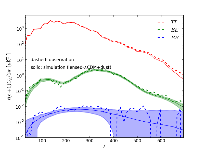
Figure 1.— Raw temperature, $E$- and $B$-mode spectra (dashed lines) measured from BK14, compared with those from lensed-$\Lambda$CDM+dust+noise simulations. (Both have been noise debiased but no beam or filtering correction has been applied.) For the simulations the solid line shows the mean value and the shaded region the $\pm 1\sigma$ range. The temperature sky input to the simulations is constrained to be the actual sky pattern as observed by Planck so there is no sample variance in the simulated $TT$ spectra.

In addition to the above filtering function, we filter in multipole space to select $E$ and $B$-modes with the baseline ranges being $30\leq\ell\leq 700$ and $150\leq\ell\leq 700$ respectively. The minimum multipole of the $E$-modes is set by the timestream filtering—multipoles smaller than $\raise 2.9pt\hbox{$\scriptstyle<$}\lower 0.5pt\hbox{$\scriptscriptstyle\sim$}\;30$ are so heavily attenuated as to be unrecoverable. The minimum multipole of the $B$-modes is chosen so that the dust foreground is subdominant compared to the lensing $B$-modes. The nominal maximum multipole is set by the resolution of the standard BK14 maps which have 0.25^∘ pixel spacing. We will see later (in Sec. V) that restricting to $\ell<600$ makes very little difference to the final result.

We have not previously published any results for $\ell>350$ because the beam correction becomes very large, and hence in principle so does the uncertainty on that correction. As shown in 1, we find that the mean of the signal simulations actually remains very close to the observed bandpower values for multipoles all the way up to the pixel scale. However there is a small positive deviation at higher $\ell$ which reaches $20\%$ at $\ell=600$ implying that we have slightly under-estimated our beam function in this range. This is very clear in the $TT$ spectrum because the input sky for the simulations is constrained to the actual sky pattern as observed by Planck (as described in Sec. V.A.1 of BK-I), and hence there is no sample variance in this comparison. Based on this observation we apply a small additional beam correction for the baseline lensing analysis presented in this paper. In practice, we multiply the inverse square root of the $\ell$-dependent correction to the observed (and also simulated noise) $E$-/$B$-modes, and then compute the weighted Fourier modes of Eq. (17). As shown in Sec. V, this correction only leads to small changes in the final results.

III.3. Estimating the lensing potential

We now describe the estimator for the lensing potential. Eq. (10) motivates the following quadratic estimator for the lensing potential (Hu, 2001; Hu & Okamoto, 2002)

$$\widehat{\phi}_{\textit{{L}}}=A_{\textit{{L}}}^{\phi}(\overline{\phi}_{\textit{{L}}}-\langle\overline{\phi}_{\textit{{L}}}\rangle)\,,$$ (18)

where $\langle\cdots\rangle$ is the ensemble average over realizations of purified $E$ and $B$ modes, and $\overline{\phi}_{\textit{{L}}}$ is the unnormalized $EB$ estimator

$$\overline{\phi}_{\textit{{L}}} ={\int\!\!\frac{\,{\rm d}^{2}\bm{\ell}\,}{(2\pi)^{2}}\,}w^{\phi}_{\textit{{L}},\bm{\ell}}\overline{E}_{\bm{\ell}}\overline{B}_{\textit{{L}}-\bm{\ell}}\,.$$ (19)

Here $w^{\phi}_{\textit{{L}},\bm{\ell}}$ is the weight function given in Eq. (11). The second term, $\langle\overline{\phi}_{\textit{{L}}}\rangle$, is a correction for the mean-field bias, and is estimated from the simulations. The quantities, $\overline{E}$ and $\overline{B}$, are the weighted Fourier modes given in Eq. (17), and $A_{\textit{{L}}}$ is a normalization that makes the estimator unbiased.

Similarly, the curl-mode estimator is constructed by replacing the weight function with $w_{\textit{{L}},\bm{\ell}}^{\varpi}$, which is given in Eq. (12). Up to first order in $\phi$ and $\varpi$, the estimator of the lensing potential is unbiased even in the presence of the curl-mode, and vice versa (Namikawa et al., 2012).

Unlike the lensing reconstruction from the temperature and $E$-mode, the mean-field bias due to the presence of the sky cut is typically small for this $EB$ estimator with an appropriate treatment for $E$/$B$ mixing (Namikawa & Takahashi, 2013; Pearson et al., 2014). Other non-lensing anisotropies could generate a mean-field component (e.g. Hanson et al. 2009), but our simulations show that the mean-field bias is smaller than the simulation noise which corresponds to $A_{L}^{\phi}$ divided by the number of realizations (see e.g. Namikawa et al. 2013). We also note again that our simulated maps are generated with the temperature sky constrained to that observed by Planck. However, the use of these constrained realizations results in a contribution in the mean-field bias which is consistent with the simulation noise, and therefore has a negligible effect on our results.

In the ideal case, the normalization of the estimator is given analytically by

$$\overline{A}_{\textit{{L}}}^{\phi} =\left\{{\int\!\!\frac{\,{\rm d}^{2}\bm{\ell}\,}{(2\pi)^{2}}\,}\frac{|w_{\textit{{L}},\bm{\ell}}^{\phi}|^{2}}{\widehat{C}^{\rm EE}_{\ell}\widehat{C}^{\rm BB}_{|\textit{{L}}-\bm{\ell}|}}\right\}^{-1}\,.$$ (20)

In BICEP / Keck, different CMB multipoles are mixed by the survey boundary and anisotropic filtering. Therefore, we calculate the normalization factor using simulations, as other experiments have done (Polarbear Collaboration 2014b; van Engelen et al. 2015; Story et al. 2015). In practice, we use the following additional normalization:

$$A_{\textit{{L}}}^{\phi}=\frac{\langle|\phi^{\rm in}_{\textit{{L}}}|^{2}\rangle}{\langle\phi^{\rm in}_{\textit{{L}}}(\widehat{\phi}_{\textit{{L}}}^{\rm sim})^{*}\rangle}\overline{A}^{\phi}_{\textit{{L}}}\,,$$ (21)

where $\phi_{\textit{{L}}}^{\rm in}$ and $\widehat{\phi}_{\textit{{L}}}^{\rm sim}$ are the input and reconstructed lensing potential from simulation.

III.4. Estimating the lensing potential power spectrum

We estimate the lensing potential power spectrum using the reconstructed lensing potential from BK14 data alone, and also by cross-correlating the reconstructed lensing potential from BK14 with that from Planck.

The power spectrum of the lensing potential is estimated by squaring $\widehat{\phi}_{\textit{{L}}}$. The lensing potential estimator is quadratic in the CMB, and its power spectrum is the four-point correlation of the CMB anisotropies. This power spectrum can be decomposed into the disconnected and connected parts

$$\langle|\widehat{\phi}_{\textit{{L}}}|^{2}\rangle=\langle|\widehat{\phi}_{\textit{{L}}}|^{2}\rangle_{\rm C}+\langle|\widehat{\phi}_{\textit{{L}}}|^{2}\rangle_{\rm D}\,.$$ (22)

The disconnected part $|\widehat{\phi}_{\textit{{L}}}|^{2}_{\rm D}$ comes from the Gaussian part of the four-point correlation, while the connected part contains the non-Gaussian contributions from lensing. The connected part gives the lensing power spectrum, $C_{L}^{\phi\phi}$, with a correction from the higher-order bias (Kesden et al., 2003) which is negligible in our analysis. On the other hand, the disconnected part of the four-point correlation remains even in the absence of lensing, and is given by

$$\langle|\widehat{\phi}|^{2}_{\textit{{L}}}\rangle_{\rm D} =(A_{L}^{\phi})^{2}{\int\!\!\frac{\,{\rm d}^{2}\bm{\ell}\,}{(2\pi)^{2}}\,}{\int\!\!\frac{\,{\rm d}^{2}\bm{\ell}^{\prime}\,}{(2\pi)^{2}}\,}w^{\phi}_{\textit{{L}},\bm{\ell}}w^{\phi}_{-\textit{{L}},\bm{\ell}^{\prime}}$$

$$\times[\overline{{\bm{\mathrm{C}}}}^{\rm EE}_{\bm{\ell},\bm{\ell}^{\prime}}\overline{{\bm{\mathrm{C}}}}^{\rm BB}_{\textit{{L}}-\bm{\ell},-\textit{{L}}-\bm{\ell}^{\prime}}+\overline{{\bm{\mathrm{C}}}}^{\rm EB}_{\bm{\ell},\textit{{L}}-\bm{\ell}^{\prime}}\overline{{\bm{\mathrm{C}}}}^{\rm EB}_{\bm{\ell}^{\prime},-\textit{{L}}-\bm{\ell}}]\,,$$ (23)

where $A_{L}^{\phi}$ is the angle average of the estimator normalization in Eq. (21), and $\overline{{\bm{\mathrm{C}}}}^{XY}_{\bm{\ell},\bm{\ell}^{\prime}}\equiv\langle\overline{X}_{\bm{\ell}}\overline{Y}_{\bm{\ell}^{\prime}}\rangle$ is the covariance matrix. The disconnected part of the four-point correlation is produced by both the CMB fluctuations and instrumental noise. We describe the treatment of the disconnected bias for auto- and cross- lensing power in the next two sections.

III.4.1 Auto-spectrum of BK14

For the auto-spectrum of the BK14 lensing potential, the disconnected bias is a significant contribution that must be subtracted. The de-biased lensing potential power spectrum is given by

$$\widehat{C}^{\phi\phi}_{\textit{{L}}}\equiv|\widehat{\phi}_{\textit{{L}}}|^{2}-\widehat{N}_{\textit{{L}}}^{\phi}\,,$$ (24)

where $\widehat{N}_{\textit{{L}}}^{\phi}$ is the disconnected bias, and a normalization factor (the correction for the apodization window) is omitted for clarity. In principle, this Gaussian bias can be estimated from the explicit formula in Eq. (23) or dedicated Gaussian simulations. However, these approaches rely on an accurate model of $\overline{{\bm{\mathrm{C}}}}^{XY}_{\bm{\ell},\bm{\ell}^{\prime}}$. Using an inaccurate covariance matrix, $\overline{{\bm{\mathrm{C}}}}^{XY}+\Sigma^{XY}$, Eq. (23) results in an error $\mathcal{O}(\Sigma^{XY})$.

In our analysis, the disconnected bias is estimated with the realization-dependent method developed by Namikawa et al. (2013) for temperature and extended by Namikawa & Takahashi (2013) to include polarization. In this method, part of the covariance is replaced with the real data, and is given by

$$\widehat{N}_{\textit{{L}}}^{\phi} =\langle|\widehat{\phi}^{E_{\bm{1}},\widehat{B}}_{\textit{{L}}}+\widehat{\phi}_{\textit{{L}}}^{\widehat{E},B_{\bm{1}}}|^{2}\rangle_{\bm{1}}-\frac{1}{2}\langle|\widehat{\phi}_{\textit{{L}}}^{E_{\bm{1}},B_{\bm{2}}}+\widehat{\phi}_{\textit{{L}}}^{E_{\bm{2}},B_{\bm{1}}}|^{2}\rangle_{\bm{1},\bm{2}}\,.$$ (25)

Here $\widehat{\phi}^{XY}_{\textit{{L}}}$ is the lensing estimator computed from the quadratic combination of $X$ and $Y$. $\widehat{E}$ and $\widehat{B}$ are the purified $E$- and $B$-modes from real data, while $E_{\bm{1}}$ ($E_{\bm{2}}$) and $B_{\bm{1}}$ ($B_{\bm{2}}$) are generated from the first (second) set of simulations. The ensemble average $\langle\cdots\rangle_{\bm{i}}$ is taken over the $i$’th set of simulations. Our simulation set is divided into two subsets multiple times to estimate the second term.

Note that this form of disconnected bias is obtained naturally from the optimal estimator for the lensing-induced trispectrum using the Edgeworth expansion of the CMB likelihood (Appendix A). Realization-dependent methods have the benefit of suppressing spurious off-diagonal elements in the covariance matrix. Furthermore, the disconnected bias estimated using this method is less sensitive to the accuracy of the covariance, i.e., it contains contributions from $\mathcal{O}(\Sigma^{2})$ instead of $\mathcal{O}(\Sigma)$.

The curl-mode power spectrum is also estimated in the same way but with the quadratic estimator of the curl-mode $\widehat{\varpi}_{\textit{{L}}}$, while the disconnected bias becomes very small in estimating the cross-spectrum between the lensing potential and curl mode.

III.4.2 Cross-spectrum with Planck

In cross-correlation studies involving Planck  we expect the disconnected bias in cross-spectra to be completely negligible. The reasons are as follows.

In cross-spectrum analysis, the instrumental noise of the two experiments is uncorrelated. Disconnected bias can only arise from sky signal. The Planck 2015 lensing potential is estimated from all of the quadratic estimators, including those involving polarization. Therefore, even in the absence of lensing, two of these quadratic estimators (the $EB$ and $TB$ estimators) are correlated with the $EB$ estimator computed from the BK14 data through the common sky signal.

In practice, this disconnected bias is small. The correlation of $B$-modes between these two experiments does not contain noise contributions. The four-point correlation, $EBEB$ and $TBEB$, are then produced by the CMB $B$-mode signals but not by the instrumental noise in $B$-modes. The uncertainties in the Planck lensing potential are dominated by instrumental noise, which is much larger than any possible $B$-modes on the sky that can lead to a disconnected bias. To see this more quantitatively, we evaluate the disconnected bias expected from the $\Lambda$CDM $B$-mode power spectrum and appropriate noise levels, using the analytic formula based on Hu & Okamoto (2002). We find that the bias is indeed negligible compared to the reconstruction noise (see 5).

In addition, since the Planck 2013 lensing potential is reconstructed from the temperature maps alone, the cross-spectrum between BK14 and Planck 2013 is free of any disconnected bias. In the next section, we show that the cross-spectrum results with Planck 2013 and Planck 2015 are consistent, again confirming that the disconnected bias in the Planck 2015 - BK14 cross-spectrum is not significant.

III.4.3 Binned power spectrum and its amplitude

In our analysis the multipoles between $30$ and $700$ are divided into $10$ bins and the bandpowers of the lensing potential power spectrum $C_{b}$ are given at these multipole bins. We estimate the amplitude of the lensing potential power spectrum as a weighted mean over multipole bins

$$A_{\rm L}^{\phi\phi}=\frac{\sum_{b}a_{b}A_{b}}{\sum_{b}a_{b}}\,,$$ (26)

where $A_{b}$ is the relative amplitude of the power spectrum compared with a fiducial power spectrum $C_{b}^{\rm f}$, i.e., $A_{b}\equiv C_{b}/C_{b}^{\rm f}$, and the weights, $a_{b}$, are taken from the bandpower covariance according to

$$a_{b}=\sum_{b^{\prime}}C^{\rm f}_{b}{\bm{\mathrm{Cov}}}_{bb^{\prime}}^{-1}C^{\rm f}_{b^{\prime}}\,.$$ (27)

The fiducial bandpower values and their covariances are evaluated from the simulations. Consequently, $A_{\rm L}^{\phi\phi}$ defined as above is an amplitude relative to the Planck $\Lambda$CDM prediction.

IV. Results

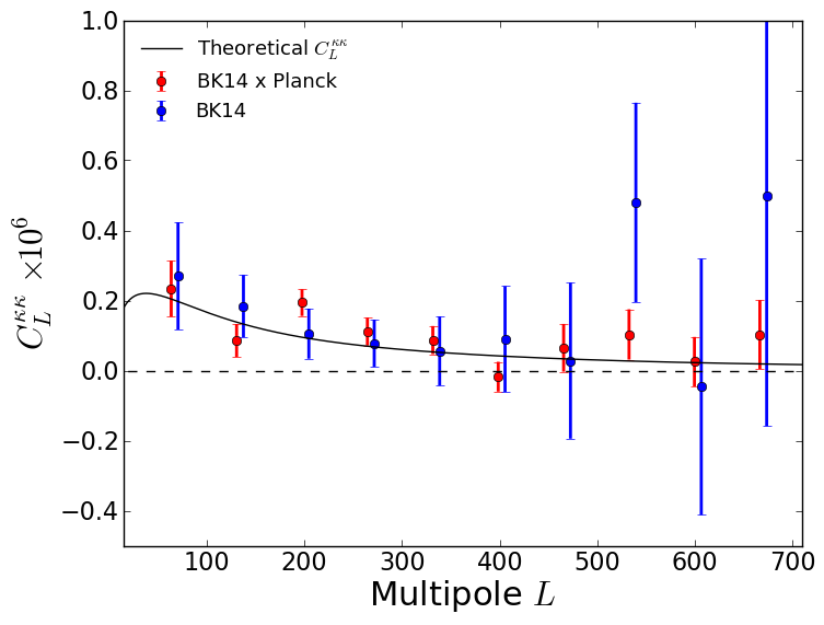
Figure 2.— The lensing-mass power spectrum, $C_{L}^{\kappa\kappa}=L^{4}C^{\phi\phi}_{L}/4$, estimated from the cross-spectrum between BK14 and Planck 2015 data (red), and the auto-spectrum of BK14 data (blue). The black solid line shows the theoretical spectrum assuming the $\Lambda$CDM cosmology. The BK14 auto-spectrum is offset in $L$ for clarity.

Table 1 The bandpowers of the lensing-mass power spectrum and $1\sigma$ statistical errors at the center of each bin, $L_{\rm c}$, as shown in 2. The values of the bandpowers and errors are multiplied by $10^{7}$.

$L_{\rm c}$	BK14$\times$Planck	BK14
$63.5$	$2.33\pm 0.80$	$2.70\pm 1.53$
$130.5$	$0.86\pm 0.47$	$1.84\pm 0.89$
$197.5$	$1.94\pm 0.38$	$1.05\pm 0.72$
$264.5$	$1.11\pm 0.40$	$0.78\pm 0.67$
$331.5$	$0.87\pm 0.40$	$0.55\pm 0.99$
$398.5$	$-0.18\pm 0.43$	$0.90\pm 1.51$
$465.5$	$0.65\pm 0.68$	$0.28\pm 2.23$
$532.5$	$1.03\pm 0.72$	$4.80\pm 2.85$
$599.5$	$0.25\pm 0.71$	$-0.47\pm 3.66$
$666.5$	$1.03\pm 0.98$	$4.97\pm 6.56$

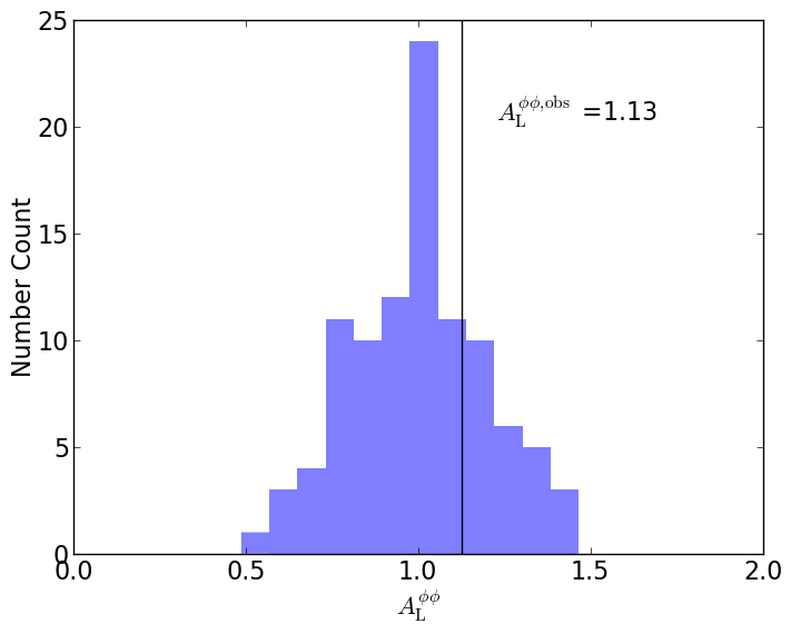
Figure 3.— The amplitudes of the cross-spectra of BK14 and Planck 2015 lensing potential maps reconstructed from lensed-$\Lambda$CDM+dust+noise simulations (histogram), and the observed value (vertical line).

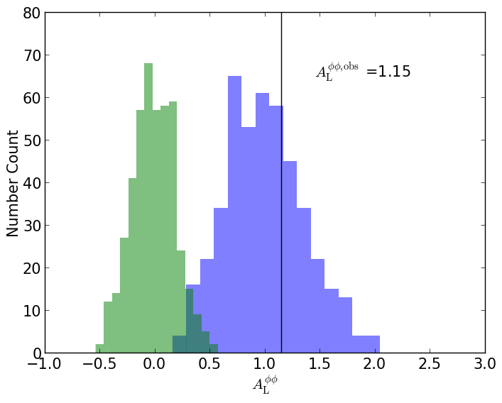
Figure 4.— The amplitudes of the auto-spectra of BK14 lensing potential maps reconstructed from lensed-$\Lambda$CDM+dust+noise simulations (blue histogram), and from unlensed-$\Lambda$CDM+dust+noise simulations (green histogram). The observed value is indicated by the vertical line.

2 shows the cross-spectrum of the BK14 and Planck lensing-mass fields, and the auto-spectrum of the BK14 data alone. Table 1 shows the bandpowers and $1\sigma$ statistical errors of the lensing power spectrum. 3 compares the amplitude of the lensing cross-spectrum between BK14 and Planck to lensed-$\Lambda$CDM+dust+noise simulations, while the line and blue histogram in 4 do the same thing for the BK14 auto-spectrum. The observed amplitude estimated from the cross-spectrum is $A_{\rm L}^{\phi\phi}=1.13\pm 0.20$ and the amplitude estimated from the auto-spectrum is $A_{\rm L}^{\phi\phi}=1.15\pm 0.36$. In each case the uncertainty is taken from the standard deviation of the lensed-$\Lambda$CDM+dust+noise simulations. We find that these values are mutually consistent, and are also consistent with the Planck $\Lambda$CDM expectation within the $1\sigma$ statistical uncertainty.

To evaluate the rejection significance of the no-lensing hypothesis in 4 we also show the results of a special set of unlensed-$\Lambda$CDM+dust+noise simulations where there is no sample variance on the lensing component. Assuming Gaussian statistics we find that the no-lensing hypothesis is rejected at $5.8\sigma$ which is the highest significance achieved to date using $EB$ lensing estimator.

The $B$-mode power spectrum can also be used to constrain the amplitude of the lensing effect and in BKP we quoted the value $A_{\rm L}^{\rm BB}=1.13\pm 0.18$ when marginalizing over $r$ and the dust foreground amplitude. Updating to the BK14 spectrum and setting $r=0$ we find $A_{\rm L}^{\rm BB}=1.20\pm 0.17$. The agreement of this result with that from the lensing reconstruction described above verifies that the $B$-mode observed by the BICEP / Keck experiments at intermediate angular scales is dominated by gravitational lensing.

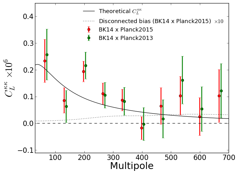
Figure 5.— The lensing-mass power spectrum, $C_{L}^{\kappa\kappa}=L^{4}C^{\phi\phi}_{L}/4$, estimated from the cross-spectrum between BK14 and Planck 2015 data compared with that between BK14 and Planck 2013 data. We also show the theoretical expectation of the disconnected bias in the cross-spectrum between the BK14 and Planck 2015 data multiplied by $10$. The cross-spectrum between BK14 and Planck 2013 is offset in $L$ for clarity.

To show that the disconnected bias in the cross-spectrum is small, an analytic estimate multiplied by 10$\times$ for clarity is compared in 5 to the BK14/Planck 2015 cross-spectrum. The inclusion of this bias changes the value of the lensing amplitude by less than $1\%$. In addition, we show an alternate cross-spectrum taken between BK14 and the Planck 2013 data. As mentioned earlier, the BK14 and Planck 2013 cross-spectrum is free of any disconnected bias. Therefore, the similarity of these two spectra also suggests that the disconnected bias in the BK14 and Planck 2015 cross-spectrum is small.

V. Consistency checks and null tests

In this section, we discuss systematics in the reconstructed lensing potential. $B$-modes in the $EB$ estimator for $\phi$ are an order of magnitude fainter than the $E$-modes, and need to be tested for non-negligible contributions from systematics or leakage from $E$-modes. The matrix-purified BK14 $E$- and $B$-modes up to $\ell\simeq 350$ used in this paper have already passed the long list of systematics and null tests described in BK-I, BK-III and BK-VI. In the baseline results presented above we include additional modes up to $\ell_{\rm max}=700$, and we see below that the modes in the range $350<\ell<600$ carry a significant portion of the total available statistical weight. In this section we therefore discuss additional tests that demonstrate the robustness of the reconstructed $\phi$ map and the lensing spectrum. Furthermore, note that the cross-spectrum of BK14 and Planck, which produces the most stringent constraint on $A_{\rm L}^{\phi\phi}$ in this paper, is immune to additive bias from all known systematics, and is highly insensitive to the dust foreground.

V.1. Null tests

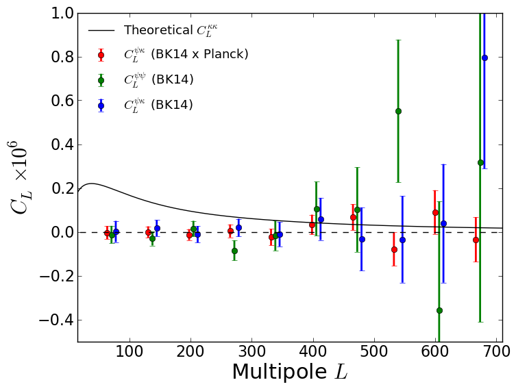
Figure 6.— Curl null test: The cross-spectrum of the curl-mode reconstructed from BK14 data and the Planck lensing-mass field (red), the auto-spectrum of the BK14 curl-mode (green), and the cross-spectrum of the BK14 lensing-mass field and curl-mode (blue). For comparison, we also show the theoretical lensing-mass power spectrum (black). The power spectra are offset in $L$ for clarity.

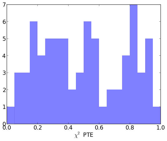
Figure 7.— Distribution of the jackknife $\chi^{2}$ PTE values.

Table 2 Probability to exceed a $\chi^{2}$ statistic for the curl null test and the jackknife tests.

	BK14 $\times$ Planck		BK14
	$\phi\times\phi$	$\varpi\times\phi$	$\phi\times\phi$	$\varpi\times\phi$	$\varpi\times\varpi$
Curl	—	0.77	—	0.92	0.34
Deck	0.51	0.48	0.34	0.06	0.12
Scan Dir	0.37	0.43	0.87	0.15	0.57
Tag Split	0.30	0.85	0.36	0.86	0.73
Tile	0.30	0.16	0.20	0.05	0.54
Phase	0.69	0.68	0.92	0.76	0.25
Mux Col	0.18	0.22	0.46	0.38	0.35
Alt Deck	0.18	0.72	0.39	0.16	0.16
Mux Row	0.49	0.80	0.60	0.58	0.09
Tile/Deck	0.20	0.36	0.83	0.84	0.88
Focal Plane inner/outer	0.09	0.12	0.41	0.35	0.28
Tile top/bottom	0.84	0.51	0.51	0.77	0.28
Tile inner/outer	0.31	0.05	0.91	0.64	0.78
Moon	0.02	0.84	0.18	0.53	0.83
A/B offset best/worst	0.93	1.00	0.57	0.24	0.59

In the following we present results of i) a curl-null test, and ii) jackknife tests, which are expected to be consistent with zero unless there are systematics remaining in the data.

To test this quantitatively, we use the probability to exceed (PTE) the value of $\chi^{2}$ obtained from observations, under the assumption that the fiducial power spectrum is zero in all multipole bins. The PTE is evaluated from the simulation set with the same method as in the BK-I paper. Table 2 summarizes the PTE values obtained. 7 shows the distribution of the jackknife $\chi^{2}$ PTE.

V.1.1 Curl null test

The curl-mode is mathematically similar to lensing but cannot be generated by scalar perturbations at linear order. As described in Sec. III, the curl-mode is estimated by replacing the weight function with $w_{\bm{\ell},\textit{{L}}}^{\varpi}$, and the reconstruction noise level in the curl-mode is similar to that in the lensing potential. It is therefore commonly used as an important check for any residual systematics in lensing reconstruction analysis.

6 shows the cross-spectrum between the BK14 curl-mode and the Planck lensing potential, the BK14 curl-mode auto-spectrum, and the cross-spectrum between the BK14 lensing potential and curl-mode. For illustrative purposes, similar to the relationship between $\kappa$ and $\phi$, we define $\psi_{\textit{{L}}}=-L^{2}\varpi_{\textit{{L}}}/2$, and show the power spectrum of $\psi$ instead of $\varpi$. We compute the corresponding PTEs for these power spectra (see Table 2), finding no evidence of systematics in these curl-null tests.

V.1.2 Jackknife tests

As part of our standard data reduction we form multiple pairs of jackknife maps which split the data into approximately equal halves, and which should contain (nearly) identical sky signal, but which might be expected to contain different systematic contamination. We then difference these pairs of maps and search for signals which are inconsistent with the noise expectation—see BK-I, BK-III and BK-VI for further details. Here we take these jackknife maps, perform the lensing reconstruction on them, and as usual look for signals which are inconsistent with null.

Table 2 gives the PTE values. We find no evidence of spurious signals in the lensing potential.

V.2. Consistency checks

Table 3 The amplitude of the lensing potential power spectrum $A_{\rm L}^{\phi\phi}$ estimated with different analysis choices.

	BK14 $\times$ Planck	BK14
Baseline	$1.13\pm 0.20$	$1.15\pm 0.36$
$\ell_{\rm max}=650$	$1.07\pm 0.20$	$1.21\pm 0.36$
$\ell_{\rm max}=600$	$1.14\pm 0.20$	$1.26\pm 0.36$
$\ell_{\rm max}=350$	$1.41\pm 0.30$	$1.97\pm 0.84$
$\ell_{\rm min}=150$	$1.13\pm 0.20$	$1.14\pm 0.36$
$\ell_{\rm min}=200$	$1.07\pm 0.20$	$0.95\pm 0.40$
$\ell_{\rm max}^{\rm B}=350$	$1.24\pm 0.22$	$1.33\pm 0.45$
Diff. beam ellipticity	$1.11\pm 0.20$	$1.14\pm 0.36$
Apodization	$1.07\pm 0.22$	$0.99\pm 0.39$

As consistency checks of the BK14 lensing potential, we calculate the lensing power spectrum while varying the following analysis choices from their baseline values, and give the resulting alternate values of $A_{\rm L}^{\phi\phi}$ in Table 3.

• Maximum multipole: $\ell_{\rm max}$
  In our baseline analysis, the nominal maximum multipole of the $E$- and $B$-modes used for the lensing reconstruction in Eq. (19) is $\ell_{\rm max}=700$. Reducing the value of $\ell_{\rm max}$ to $650$ and $600$ we see small changes in the constraint on $A_{\rm L}^{\phi\phi}$. However, if we reduce $\ell_{\rm max}$ to $350$ to match the range probed by jackknife tests in BK-VI, the values of $A_{\rm L}^{\phi\phi}$ shift up, and the statistical errors increase. To quantify how likely the up-shifts are to occur by chance we compute the corresponding shifts when making the same change in the simulations, and find a positive shift greater than the observed one $10$% of the time for the cross-spectrum and $15$% of the time for the auto-spectrum.

• Minimum multipole: $\ell_{\rm min}$
  For the baseline analysis the minimum multipole of the $E$-modes is set to $30$ in Eq. (19) (due to the timestream filtering), while the minimum multipole of the $B$-modes is set to $150$ (to ensure that the contributions of the dust foreground is small compared to the noise and lensing signal). Raising $\ell_{\rm min}$ for the $E$-modes to $150$ we see very small changes to the $A_{\rm L}^{\phi\phi}$ results, while raising both to $200$ we see modest changes.

• Maximum multipole of the $B$-mode polarization: $\ell_{\rm max}^{\rm B}$
  As mentioned above, $B$-modes are used up to a nominal $\ell_{\rm max}=700$ in our baseline analysis. The $B$-mode polarization at $\ell\gtrsim 350$ is not as well tested against various systematics. However, unlike $E$-modes, $B$-modes at smaller scales $\ell>350$ do not contribute significantly in estimating $A_{\rm L}^{\phi\phi}$. We repeat the analysis removing $B$-modes at $\ell>350$, and find only a moderate change in the results and their statistical uncertainties.

• Differential beam ellipticity:
  In our pair-differencing analysis differences in the beam shapes between the A and B detectors of each pair generates temperature-to-polarization leakage. We filter out the leading order modes of this leakage using a technique which we call deprojection (see BK-III for details). For differential beam ellipticity, however, we do not use deprojection because it introduces a bias in $TE$. Instead, in our standard analysis, we subtract the expected temperature-to-polarization leakage based on the measured differential beam ellipticity. To test whether the lensing results are sensitive to differential beam ellipticity, we repeat the lensing reconstruction from maps without this subtraction and find only a very small change in the results.

• Apodization:
  To mitigate the noisy regions around the survey boundary, after obtaining the purified $E$ and $B$ modes, our standard analysis applies an inverse variance apodization window. We also perform the analysis using the sine apodization defined in Namikawa & Takahashi (2013) and find only a small change in the results.

V.3. Effects of beam systematics

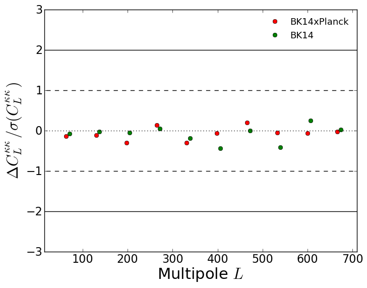
Figure 8.— The difference of the lensing power spectrum when subtracting from the BK14 $Q/U$ maps a nominal undeprojected residual as derived from per-channel beam maps (red: BK14$\times$Planck, blue:BK14), divided by the $1\,\sigma$ statistical uncertainty.

Beam shape mismatch of each detector pair leads to a leakage from the bright temperature anisotropies into polarization (e.g. Hu et al. 2003; Miller et al. 2008; Su et al. 2009). In our analysis, this leakage is mitigated by deprojecting (or for ellipticity, subtracting) several modes corresponding approximately to the difference of two elliptical Gaussians (see BK-III for details). To assess the level of leakage remaining after deprojection, we use calibration data consisting of high precision, per-detector beam maps described in BK-IV. In special simulations, we explicitly convolve these beam maps onto an input $T$ sky and process the resulting simulated timestream in the normal manner, including deprojection, to produce maps of the “undeprojected residual.” In BK-V, this residual was treated as an upper limit to possible residual systematics. Here, as an additional check, we try subtracting this nominal residual from the maps and re-extracting the lensing potential. 8 shows the differences in the resulting spectrum in units of the bandpower uncertainties, finding that the difference is small compared to the $1\,\sigma$ statistical uncertainty.

In addition to temperature-to-polarization leakage caused by beam mismatch, beam asymmetry as well as detector-to-detector beam shape variation can produce a spurious lensing signal if non-uniform map coverage leads to an effective beam that is spatially dependent (e.g. Planck Collaboration 2014a). The beam map simulation procedure described above does not probe this effect in the $EB$ estimator because the input maps do not contain polarization. However, we note that ellipticity is the dominant component of beam asymmetry and beam shape variation in BICEP2 and Keck (see BK-IV, Table 2). We also note that beam ellipticity is a strong function of radial position in the focal plane (see BK-IV, Figures 12-13), so that the focal plane inner/outer jackknife listed in Table 2 is a good proxy for a beam ellipticity jackknife. The fact that this null test passes limits the contribution from beam asymmetry and beam variation to less than the uncertainty.

We finally test the effects of the beam correction to $E$-/$B$-modes based on the observed level of temperature anisotropies at high $\ell$ (Sec. III). We repeat the same lensing reconstruction without the beam correction, and estimate the lensing amplitude. We find that $A_{\rm L}^{\phi\phi}$ increases while the statistical error is unchanged compared to the baseline results, and the differences of $A_{\rm L}^{\phi\phi}$ are $\Delta A_{\rm L}^{\phi\phi}=0.05$ for BK14$\times$ Planck and $\Delta A_{\rm L}^{\phi\phi}=0.15$ for BK14. These changes are within the $1\sigma$ statistical error.

V.4. Effects of absolute calibration error

Although the lensing potential is in principle a dimensionless quantity, the measured lensing potential depends on the overall amplitude of the polarization map. The calibration uncertainties in $E$- and $B$-modes therefore propagate into an error in the amplitude of the lensing potential spectrum (e.g. Polarbear Collaboration 2014b). The absolute calibration uncertainty, $\delta$, is $1.3$% in the BICEP2/Keck polarization maps (BK-I). Given this uncertainty on amplitudes of the $E$- and $B$-modes, the resultant systematic uncertainties in the lensing spectral amplitudes are $\Delta A_{\rm L}^{\phi\phi}=4\delta=0.052$ for the BK14 auto-spectrum and $\Delta A_{\rm L}^{\phi\phi}=2\delta=0.026$ for the cross-spectrum with Planck, significantly smaller than the statistical uncertainties. Since the estimate of the curl-mode power spectrum is also affected in the same manner, non-detection of the curl mode also indicates that the effect of these uncertainties is negligible compared to the statistical errors.

VI. Conclusions

In this paper we have reconstructed the lensing potential from the BK14 polarization data, and taken its cross-spectrum with the public Planck lensing potential, as well as the auto-spectrum of the BK14 alone. The amplitude of the cross-spectrum with Planck is constrained to be $A_{\rm L}^{\phi\phi}=1.13\pm 0.20$, while the auto-spectrum has amplitude $A_{\rm L}^{\phi\phi}=1.15\pm 0.36$. By comparing the auto-spectrum to special unlensed simulations we reject the no-lensing hypothesis at $5.8\sigma$ significance, which is the highest significance achieved to date using $EB$ lensing estimator. We have performed several consistency checks and null tests, and find no evidence for spurious signals in our reconstructed map and spectra.

This paper demonstrates for the first time lensing reconstruction using $B$-modes in the intermediate multipole range. The results verify that the $B$-mode power observed by the BICEP / Keck experiments on these intermediate angular scales is dominated by gravitational lensing. The good agreement between these results and $A_{\rm L}^{\rm BB}=1.20\pm 0.17$ from the BK14 $B$-mode spectrum starts to place constraints on any alternative sources of $B$-modes at these angular scales, such as cosmic strings (e.g., Seljak & Slosar 2006; Pogosian & Wyman 2008), primordial magnetic fields (e.g., Shaw & Lewis 2010; Bonvin et al. 2014) and cosmic birefringence induced by interaction between a massless pseudo-scalar field and photons (e.g., Pospelov et al. 2009; Lee et al. 2015; Polarbear Collaboration 2015). The calculation of formal quantitative constraints is rather involved and depends on the assumed statistical properties of the alternative $B$-mode sources. We leave that to future work.

Looking ahead, the reconstructed lensing potential can be used to cross-correlate with other astronomical tracers. However, the reconstruction noise of the BICEP / Keck data will limit its usefulness as a cosmological probe in the era of DES (The Dark Energy Survey Collaboration, 2016), DESI (The DESI Collaboration, 2013), and LSST (LSST Dark Energy Science Collaboration, 2012). As the sensitivity of BICEP / Keck improves, our main objective is to use a well-measured deflection map $\phi$ to form a degree-scale $B$-mode lensing template, which can then be used to improve our final uncertainties on $r$ (i.e., “delensing”). Multiple studies have shown that high resolution CMB polarization data (e.g., Seljak & Hirata 2004; Smith et al. 2012), the CIB (Simard et al., 2015; Sherwin & Schmittfull, 2015), galaxy clustering (Namikawa et al., 2016), or weak lensing (Sigurdson & Cooray, 2005; Marian & Bernstein, 2007) can all improve measurements of $\phi$. In addition to the lensing potential presented here there already exists in the BICEP / Keck field data from the Planck CIB measurements (Planck Collaboration, 2014b, c), as well as high resolution CMB maps from SPTpol. We are exploring the formation of a lensing template using an optimal combination of these and anticipate using this in our likelihood analysis in the near future. This template will considerably improve as SPT3G(Benson et al., 2014) comes online.

Appendix A Disconnected bias estimation

The realization-dependent method for the disconnected bias given in Eq. (A6) comes naturally from deriving the optimal estimator for the lensing-induced trispectrum. Here we briefly summarize derivation of Eq. (A6) (see appendix A of Namikawa & Takahashi 2013 for a thorough derivation).

The lensing-induced trispectrum which is relevant to our analysis is given by (see e.g. Lewis & Challinor 2006)

$$T_{\bm{\ell}_{1}\bm{\ell}_{2}\bm{\ell}_{3}\bm{\ell}_{4}}\equiv\langle E_{\bm{\ell}_{1}}B_{\bm{\ell}_{2}}E_{\bm{\ell}_{3}}B_{\bm{\ell}_{4}}\rangle_{\rm C}\simeq\delta^{D}_{\bm{\ell}_{1}+\bm{\ell}_{2}+\bm{\ell}_{3}+\bm{\ell}_{4}}[w^{\phi}_{\bm{\ell}_{1}+\bm{\ell}_{2},\bm{\ell}_{1}}w^{\phi}_{\bm{\ell}_{3}+\bm{\ell}_{4},\bm{\ell}_{3}}C_{|\bm{\ell}_{1}+\bm{\ell}_{2}|}^{\phi\phi}+w^{\phi}_{\bm{\ell}_{1}+\bm{\ell}_{4},\bm{\ell}_{1}}w^{\phi}_{\bm{\ell}_{2}+\bm{\ell}_{3},\bm{\ell}_{2}}C_{|\bm{\ell}_{1}+\bm{\ell}_{4}|}^{\phi\phi}]\,,$$ (A1)

where $w^{\phi}_{\textit{{L}},\bm{\ell}}$ is given in Eq. (11), $C_{L}^{\phi\phi}$ is the lensing potential power spectrum, and $\delta^{D}_{\textit{{L}}}$ is the Dirac delta function in Fourier space. In the Edgeworth expansion of the $E$- and $B$-mode likelihood, the term containing the above trispectrum is given by (Regan et al., 2010)

$$\mathcal{L}\propto\left[\prod_{i=1}^{4}{\int\!\!\frac{\,{\rm d}^{2}\bm{\ell}_{i}\,}{(2\pi)^{2}}\,}\right]T_{\bm{\ell}_{1}\bm{\ell}_{2}\bm{\ell}_{3}\bm{\ell}_{4}}\dfrac{\partial}{\partial E_{\bm{\ell}_{1}}}\dfrac{\partial}{\partial B_{\bm{\ell}_{2}}}\dfrac{\partial}{\partial E_{\bm{\ell}_{3}}}\dfrac{\partial}{\partial B_{\bm{\ell}_{4}}}\mathcal{L}_{\rm g}\,,$$ (A2)

where $\mathcal{L}_{\rm g}$ is the Gaussian likelihood of the $E$- and $B$-mode:

$$\mathcal{L}_{\rm g}\propto\exp\left(-\frac{1}{2}\left[\prod_{i=1}^{2}{\int\!\!\frac{\,{\rm d}^{2}\bm{\ell}_{i}\,}{(2\pi)^{2}}\,}\right]\sum_{a,b=E,B}a_{\bm{\ell}_{1}}\{{\bm{\mathrm{C}}}^{-1}\}^{a_{\bm{\ell}_{1}}b_{\bm{\ell}_{2}}}b_{\bm{\ell}_{2}}\right)\,.$$ (A3)

Here $\{{\bm{\mathrm{C}}}\}^{a_{\bm{\ell}}b_{\bm{\ell}}}=\langle a_{\bm{\ell}}b_{\bm{\ell}^{\prime}}\rangle$ is the covariance matrix, and we omit the normalization of the above Gaussian likelihood.

The optimal estimator for the lensing power spectrum in the trispectrum is obtained by maximizing the CMB likelihood. The approximate formula which is numerically tractable is proportional to the derivative of the log-likelihood with respect to $C_{L}^{\phi\phi}$. The derivative of the above likelihood with respect to the lensing potential power spectrum is given by (Namikawa & Takahashi, 2013)

$$\dfrac{\partial\mathcal{L}}{\partial C^{\phi\phi}_{L}}\propto\left[\prod_{i=1}^{2}{\int\!\!\frac{\,{\rm d}^{2}\bm{\ell}_{i}\,}{(2\pi)^{2}}\,}\right]w^{\phi}_{\textit{{L}},\bm{\ell}_{1}}w^{\phi}_{-\textit{{L}},\bm{\ell}_{2}}\dfrac{\partial}{\partial E_{\bm{\ell}_{1}}}\dfrac{\partial}{\partial B_{\textit{{L}}-\bm{\ell}_{1}}}\dfrac{\partial}{\partial E_{\bm{\ell}_{2}}}\dfrac{\partial}{\partial B_{-\textit{{L}}-\bm{\ell}_{2}}}\mathcal{L}_{\rm g}\simeq\left(|\overline{\phi}^{EB}_{\textit{{L}}}|^{2}-\frac{\widehat{N}^{\phi}_{\textit{{L}}}}{(A^{\phi}_{\textit{{L}}})^{2}}\right)\mathcal{L}_{\rm g}\,.$$ (A4)

After correcting the normalization for the unbiased estimator, the above equations leads to Eq. (24).

Realization-dependent methods are useful to suppress spurious off-diagonal elements in the covariance matrix of the power spectrum estimates (e.g., Dvorkin & Smith 2009; Hanson et al. 2011). As discussed in Namikawa et al. (2013), the disconnected bias estimation described above is less sensitive to errors in covariance compared to the other approaches. To see this, using Eq. (18), we rewrite Eq. (23) as

$$\widehat{N}_{\textit{{L}}}^{\phi} =(A^{\phi}_{\textit{{L}}})^{2}{\int\!\!\frac{\,{\rm d}^{2}\bm{\ell}\,}{(2\pi)^{2}}\,}{\int\!\!\frac{\,{\rm d}^{2}\bm{\ell}^{\prime}\,}{(2\pi)^{2}}\,}w^{\phi}_{\textit{{L}},\bm{\ell}}w^{\phi}_{-\textit{{L}},\bm{\ell}^{\prime}}\bigg{[}\overline{{\bm{\mathrm{C}}}}^{\rm EE}_{\bm{\ell},\bm{\ell}^{\prime}}\overline{B}_{\textit{{L}}-\bm{\ell}}\overline{B}_{-\textit{{L}}-\bm{\ell}^{\prime}}+\overline{{\bm{\mathrm{C}}}}^{\rm BB}_{\textit{{L}}-\bm{\ell},-\textit{{L}}-\bm{\ell}^{\prime}}\overline{E}_{\bm{\ell}}\overline{E}_{\bm{\ell}^{\prime}}-\overline{{\bm{\mathrm{C}}}}^{\rm EE}_{\bm{\ell},\bm{\ell}^{\prime}}\overline{{\bm{\mathrm{C}}}}^{\rm BB}_{\textit{{L}}-\bm{\ell},-\textit{{L}}-\bm{\ell}^{\prime}}$$

$$\qquad+\overline{{\bm{\mathrm{C}}}}^{\rm EB}_{\bm{\ell}^{\prime},\textit{{L}}-\bm{\ell}}\overline{E}_{\bm{\ell}}\overline{B}_{-\textit{{L}}-\bm{\ell}^{\prime}}+\overline{{\bm{\mathrm{C}}}}^{\rm EB}_{\bm{\ell},-\textit{{L}}-\bm{\ell}^{\prime}}\overline{E}_{\bm{\ell}^{\prime}}\overline{B}_{\textit{{L}}-\bm{\ell}}-\overline{{\bm{\mathrm{C}}}}^{\rm EB}_{\bm{\ell},-\textit{{L}}-\bm{\ell}^{\prime}}\overline{{\bm{\mathrm{C}}}}^{\rm EB}_{\bm{\ell}^{\prime},\textit{{L}}-\bm{\ell}}\bigg{]}\,.$$ (A5)

For example, replacing the covariance matrix with an incorrect covariance model, $\overline{{\bm{\mathrm{C}}}}^{\rm EE}+\Sigma^{\rm EE}$, we obtain

$$\widehat{N}_{\textit{{L}}}^{\phi} =(A^{\phi}_{\textit{{L}}})^{2}{\int\!\!\frac{\,{\rm d}^{2}\bm{\ell}\,}{(2\pi)^{2}}\,}{\int\!\!\frac{\,{\rm d}^{2}\bm{\ell}^{\prime}\,}{(2\pi)^{2}}\,}w^{\phi}_{\textit{{L}},\bm{\ell}}w^{\phi}_{-\textit{{L}},\bm{\ell}^{\prime}}\Sigma^{\rm EE}_{\bm{\ell},\bm{\ell}^{\prime}}(\overline{B}_{\textit{{L}}-\bm{\ell}}\overline{B}_{-\textit{{L}}-\bm{\ell}^{\prime}}-\overline{{\bm{\mathrm{C}}}}^{\rm BB}_{\textit{{L}}-\bm{\ell},-\textit{{L}}-\bm{\ell}^{\prime}})+\mathcal{O}([\Sigma^{\rm EE}]^{2})\,.$$ (A6)

and $\langle\widehat{N}_{\textit{{L}}}^{\phi}\rangle$ has no contribution from $\mathcal{O}(\Sigma^{\rm EE})$.

Note that the estimators for $C_{L}^{\varpi\varpi}$ and $C_{L}^{\phi\varpi}$ are also derived in the same way (Namikawa & Takahashi, 2013). The estimator for the curl-mode power spectrum is given by replacing $\widehat{\phi}_{\textit{{L}}}$ with $\widehat{\varpi}_{\textit{{L}}}$, while the disconnected bias for $C_{L}^{\phi\varpi}$ is estimated from

$$\widehat{N}^{\phi\varpi}_{\textit{{L}}}=\langle\Re[(\widehat{\phi}^{E_{\bm{1}},\widehat{B}}_{\textit{{L}}}+\widehat{\phi}^{\widehat{E},B_{\bm{1}}}_{\textit{{L}}})(\widehat{\varpi}^{E_{\bm{1}},\widehat{B}}_{\textit{{L}}}+\widehat{\varpi}^{\widehat{E},B_{\bm{1}}}_{\textit{{L}}})^{*}]\rangle_{\bm{1}}-\frac{1}{2}\langle\Re[(\widehat{\phi}^{E_{\bm{1}},B_{\bm{2}}}_{\textit{{L}}}+\widehat{\phi}^{E_{\bm{2}},B_{\bm{1}}}_{\textit{{L}}})(\widehat{\varpi}^{E_{\bm{1}},B_{\bm{2}}}_{\textit{{L}}}+\widehat{\varpi}^{E_{\bm{2}},B_{\bm{1}}}_{\textit{{L}}})^{*}]\rangle_{\bm{1},2}\,.$$ (A7)

References

- Abazajian et al. (2015) Abazajian, K. N., et al. 2015, Astropart. Phys., 63, 66
- Allison et al. (2015) Allison, R., et al. 2015, Phys. Rev. D, 92, 123535
- Benson et al. (2014) Benson, B. A., et al. 2014, arXiv:1407.2973
- Bicep2 and Planck Collaborations (2015) Bicep2 and Planck Collaborations. 2015, Phys. Rev. Lett., 114, 101301
- Bicep2 Collaboration I (2014) Bicep2 Collaboration I. 2014, Phys. Rev. Lett., 112, 241101
- Bicep2 Collaboration II (2014) Bicep2 Collaboration II. 2014, ApJ, 792, 62
- Bicep2 Collaboration III (2015) Bicep2 Collaboration III. 2015, ApJ, 814, 110
- Bicep2 Collaboration IV (2015) Bicep2 Collaboration IV. 2015, ApJ, 806, 206
- Bicep2 / Keck Array Collaborations V (2015) Bicep2 / Keck Array Collaborations V. 2015, ApJ, 126, 811
- Bicep2 / Keck Array Collaboration VI (2015) Bicep2 / Keck Array Collaboration VI. 2015, Phys. Rev. Lett., 116, 031302
- Bicep2 / Keck Array Collaboration VII (2016) Bicep2 / Keck Array Collaboration VII. 2016, arXiv:1603.05976
- Bonvin et al. (2014) Bonvin, C., Durrer, R., & Maartens, R. 2014, Phys. Rev. Lett., 112, 191303
- Cooray et al. (2005) Cooray, A., Kamionkowski, M., & Caldwell, R. R. 2005, Phys. Rev. D, 71, 123527
- Das et al. (2011) Das, S., et al. 2011, Phys. Rev. Lett., 107, 021301
- Das et al. (2014) —. 2014, J. Cosmol. Astropart. Phys., 04, 014
- Dvorkin & Smith (2009) Dvorkin, C., & Smith, K. M. 2009, Phys. Rev. D, 79, 043003
- Giannantonio et al. (2015) Giannantonio, T., et al. 2015, MNRAS, 456, 3213
- Hanson et al. (2011) Hanson, D., Challinor, A., Efstathiou, G., & Bielewicz, P. 2011, Phys. Rev. D, 83, 043005
- Hanson et al. (2010) Hanson, D., Challinor, A., & Lewis, A. 2010, Gen. Relativ. Gravit., 42, 2197
- Hanson & Lewis (2009) Hanson, D., & Lewis, A. 2009, Phys. Rev. D, 80, 063004
- Hanson et al. (2009) Hanson, D., Rocha, G., & Gorski, K. 2009, MNRAS, 400, 2169
- Hanson et al. (2013) Hanson, D., et al. 2013, Phys. Rev. Lett., 111, 141301
- Hirata & Seljak (2003a) Hirata, C. M., & Seljak, U. 2003a, Phys. Rev. D, 67, 043001
- Hirata & Seljak (2003b) —. 2003b, Phys. Rev. D, 68, 083002
- Hu (2001) Hu, W. 2001, ApJ, 557, L79
- Hu (2002) —. 2002, Phys. Rev. D, 65, 023003
- Hu et al. (2003) Hu, W., Hedman, M., & Zaldarriaga, M. 2003, Phys. Rev. D, 67, 043004
- Hu & Okamoto (2002) Hu, W., & Okamoto, T. 2002, ApJ, 574, 566
- Kesden et al. (2002) Kesden, M. H., Cooray, A., & Kamionkowski, M. 2002, Phys. Rev. Lett., 89, 011304
- Kesden et al. (2003) —. 2003, Phys. Rev. D, 67, 123507
- Kirk et al. (2015) Kirk, D., Omori, Y., et al. 2015, arXiv:1512.04535
- Knox & Song (2002) Knox, L., & Song, Y.-S. 2002, Phys. Rev. Lett., 89, 011303
- Lee et al. (2015) Lee, S., Liu, G.-C., & Ng, K.-W. 2015, Phys. Lett. B, 746, 406
- Lewis (2005) Lewis, A. 2005, Phys. Rev. D, 71, 083008
- Lewis & Challinor (2006) Lewis, A., & Challinor, A. 2006, Phys. Rep., 429, 1
- Lewis et al. (2011) Lewis, A., Challinor, A., & Hanson, D. 2011, J. Cosmol. Astropart. Phys., 03, 018
- LSST Dark Energy Science Collaboration (2012) LSST Dark Energy Science Collaboration. 2012, arXiv:1211.0310
- Marian & Bernstein (2007) Marian, L., & Bernstein, G. M. 2007, Phys. Rev. D, 76, 123009
- Miller et al. (2008) Miller, N. J., Shimon, M., & Keating, B. G. 2008, Phys. Rev. D, 79, 063008
- Namikawa et al. (2013) Namikawa, T., Hanson, D., & Takahashi, R. 2013, MNRAS, 431, 609
- Namikawa et al. (2010) Namikawa, T., Saito, S., & Taruya, A. 2010, J. Cosmol. Astropart. Phys., 12, 027
- Namikawa & Takahashi (2013) Namikawa, T., & Takahashi, R. 2013, MNRAS, 438, 1507
- Namikawa et al. (2016) Namikawa, T., Yamauchi, D., Sherwin, D., & Nagata, R. 2016, Phys. Rev. D, 93, 043527
- Namikawa et al. (2012) Namikawa, T., Yamauchi, D., & Taruya, A. 2012, J. Cosmol. Astropart. Phys., 1201, 007
- Pan & Knox (2015) Pan, Z., & Knox, L. 2015, MNRAS, 454, 3200
- Pearson et al. (2014) Pearson, R., Sherwin, B., & Lewis, A. 2014, Phys. Rev. D, 90, 023539
- Planck Collaboration (2014a) Planck Collaboration. 2014a, A&A, 571, A17
- Planck Collaboration (2014b) —. 2014b, A&A, A18
- Planck Collaboration (2014c) —. 2014c, A&A, A30
- Planck Collaboration (2015) —. 2015, arXiv:1502.01591
- Pogosian & Wyman (2008) Pogosian, L., & Wyman, M. 2008, Phys. Rev. D, 77, 083509
- Polarbear Collaboration (2014a) Polarbear Collaboration. 2014a, Phys. Rev. Lett., 112, 131302
- Polarbear Collaboration (2014b) —. 2014b, Phys. Rev. Lett., 113, 021301
- Polarbear Collaboration (2015) —. 2015, Phys. Rev. D, 92, 123509
- Pospelov et al. (2009) Pospelov, M., Ritz, A., & Skordis, C. 2009, Phys. Rev. Lett., 103, 051302
- Pratten & Lewis (2016) Pratten, G., & Lewis, A. 2016, arXiv:1605.05662
- Regan et al. (2010) Regan, D., Shellard, E., & Fergusson, J. 2010, Phys. Rev. D, 82, 023520
- Saga et al. (2015) Saga, S., Yamauchi, D., & Ichiki, K. 2015, Phys. Rev. D, 92, 063533
- Seljak & Hirata (2004) Seljak, U., & Hirata, C. M. 2004, Phys. Rev. D, 69, 043005
- Seljak & Slosar (2006) Seljak, U., & Slosar, A. 2006, Phys. Rev. D, 74, 063523
- Shaw & Lewis (2010) Shaw, J. R., & Lewis, A. 2010, Phys. Rev. D, 81, 043517
- Sherwin & Schmittfull (2015) Sherwin, B. D., & Schmittfull, M. 2015, Phys. Rev. D, 92, 043005
- Sigurdson & Cooray (2005) Sigurdson, K., & Cooray, A. 2005, Phys. Rev. Lett., 95, 211303
- Simard et al. (2015) Simard, G., Hanson, D., & Holder, G. 2015, ApJ, 807, 166
- Smith et al. (2007) Smith, K. M., Zahn, O., & Dore, O. 2007, Phys. Rev. D, 76, 043510
- Smith et al. (2012) Smith, K. M., et al. 2012, J. Cosmol. Astropart. Phys., 1206, 014
- Story et al. (2015) Story, K. T., et al. 2015, ApJ, 810, 50
- Su et al. (2009) Su, M., Yadav, A. P. S., & Zaldarriaga, M. 2009, Phys. Rev. D, 79, 123002
- The Dark Energy Survey Collaboration (2016) The Dark Energy Survey Collaboration. 2016, MNRAS, 1601.00329
- The DESI Collaboration (2013) The DESI Collaboration. 2013, arXiv:1308.0847
- Tolan (2014) Tolan, J. E. 2014, PhD thesis
- van Engelen et al. (2012) van Engelen, A., et al. 2012, ApJ, 756, 142
- van Engelen et al. (2015) —. 2015, ApJ, 808, 9
- Wu et al. (2014) Wu, W. L. K., Errard, J., Dvorkin, C., et al. 2014, ApJ, 788, 19
- Zaldarriaga & Seljak (1998) Zaldarriaga, M., & Seljak, U. 1998, Phys. Rev. D, 58, 023003