Distributed Graphical Simulation in the Cloud

Abstract

Graphical simulations are a cornerstone of modern media and films. But existing software packages are designed to run on HPC nodes, and perform poorly in the computing cloud. These simulations have complex data access patterns over complex data structures, and mutate data arbitrarily, and so are a poor fit for existing cloud computing systems. We describe a software architecture for running graphical simulations in the cloud that decouples control logic, computations and data exchanges. This allows a central controller to balance load by redistributing computations, and recover from failures. Evaluations show that the architecture can run existing, state-of-the-art simulations in the presence of stragglers and failures, thereby enabling this large class of applications to use the computing cloud for the first time.

200(110,87)

1 Introduction

Graphical simulation is a staple of modern digital entertainment. When we see a river flow in the movie Brave, an explosion in Star Wars: Revenge of the Sith, or smoke billowing from destroyed buildings in Man of Steel, we see the result of computationally simulating fluids: water, fire, and smoke.

Being able to run simulations in the cloud would enable studios to elastically scale their simulation infrastructure when needed, such as during final production, when each shot has its final render. Graphical simulation software packages are designed to run on a single powerful server or small, 3-4 node high performance computing clusters with InfiniBand inf as their interconnect. The techniques and algorithms these simulations use work poorly in the cloud. They assume that all nodes can communicate equally, all nodes run at exactly the same speed, and failures are very rare (e.g., $<1$ in 40,000 in a multi-day simulation). They evenly partition the simulation across all of the cores used, so the simulation runs as fast as the slowest core. To handle rare failures, they use expensive and infrequent checkpointing mechanisms. Furthermore, parallel nodes run in lockstep, such that the high latency of Ethernet (100 microseconds, rather than 500 nanoseconds with InfiniBand) causes cores to fall idle during communications.

Graphical simulations require very different data and execution models than what current cloud computing systems provide. A graphical simulation uses multiple complex data models, such as a marker-and-cell grid Harlow et al. [1965] for the fluid volume, a dense particle field for the fluid surface Enright et al. [2002], and a system of linear equations to ensure fluid does not disappear. These data structures are geometric in nature and computations on neighboring regions have tight dependencies. A simulation involves a loop of many iterations that advance time. All simulation state is held in memory, as I/O is far too slow. These requirements differ greatly from data tuples as in MapReduce Dean and Ghemawat [2008], Spark Zaharia et al. [2010], and Naiad Murray et al. [2013] or graphs as in Pregel Malewicz et al. [2010] and PowerGraph Gonzalez et al. [2012].

This paper presents Nimbus, a system for running graphical simulations in the computing cloud. To deal with the scheduling challenges inherent to cloud systems, Nimbus, like other cloud systems, uses a centralized controller node that is responsible for monitoring the entire state of the simulation. To enable dynamic load balancing, Nimbus decouples data exchange and the simulation execution plan. The system runtime is responsible for data exchanges between nodes, and invoking a simulation function after all its data is ready. This decoupling gives Nimbus the ability to place data and computation based on global knowledge of the system. To make applications tolerant to node failures, the controller continuously monitors progress and dynamically inserts check-points to save data, as needed.

The next section provides an overview of graphical simulations, which motivates a set of requirements for a system to support them in the cloud. Section 3 presents a system design whose abstractions meet these requirements. Section 4 details implementation, and. Section 5 evaluates how the system handles stragglers and node failures. Section 6 and Section 7 conclude with related work and a set of open questions for future work.

2 Graphical Simulations

Graphical simulations use different data models and algorithms than what available cloud frameworks provide. This section gives an overview of the principal methods and algorithms used in graphical simulations, and explains the challenges of distributing these computations over multiple nodes. The nature of these simulations and the associated challenges motivate a set of system design requirements (§3).

As a concrete example of a graphical simulation, we focus on PhysBAM phy , an open source physics based software package for fluid and rigid body simulations. Movie studios such as ILM and Pixar use PhysBAM in production films, and the developers have won two Academy Awards for its contributions to special effects osc . PhysBAM can simulate a huge range of phenomena, but in the rest of this paper, we focus on a water simulation. Water simulation is a canonical example, as it is extremely difficult and employs methods that are required for other fluid simulations such as smoke and fire.

2.1 Fluid Models and Simulation Algorithms

There are two basic ways to computationally represent a fluid: a grid or particles. A grid divides simulated volume into cells. Per-cell state describes the state of the simulation, such as whether it contains fluid, pressure, and velocity. The second approach is to represent the fluid as a set of particles, each of which has its own $(x,y,z)$ coordinates, velocity, and size. Grids and particles have different strengths and weaknesses. For example, a grid smoothes out small ripples but do not model splashes well, while particles have difficulty representing fixed boundaries such as the edge of a glass.

The particle-levelset method Enright et al. [2002], pioneered by PhysBAM, combines particle and grid representations and is why movie and special effect studios can simulate water, smoke, and fire today. The key insight is that the most important visual feature is the surface of the fluid. The particle level-set method use a coarse grid, augmented with dense particles only on the surface. Combining these two methods, however makes simulations much more complex, as the grids and particles interact in subtle and interesting ways.

A simulation is a loop: each iteration steps time forward.  When time passes a frame boundary, the simulation outputs the visual state of the simulation for later rending. An iteration has 22 distinct computational steps, which can be divided into three major categories: updating grid cells, updating particles, and solving a set of linear equations that enforce physical laws on the water (e.g., it does not compress or disappear). Solving the linear equations uses a sub-loop within the main loop. In a typical $256^{3}$ water simulation, there are on average 20 main loop iterations per frame (24fps means 42ms/frame, the main loop time step is 1.6ms) and 100 iterations of the inner solver loop. Table 1 shows where a time step spends its time.

2.2 Current Distributed Simulations

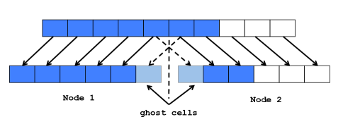
Figure 1: A 1D row of water represented in a grid. When partitioned across two processes, the two processes must exchange ghost cells of state so they can perform computations locally.

Running a simulation across multiple nodes requires partitioning the simulation geometry across them. The basic challenge is that partitions are not independent. The state of water at any cell is dependent on its neighboring cells, some of which may be on a different node. Furthermore, solving the linear equations involve global operations.

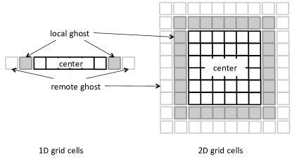
Figure 2: Ghost cell configurations in simulation grids. The local state on a node consists of $3^{d}$ objects, where $d$ is the dimensionality of the grid, while the combined local and remote state a node must use consists of $5^{d}$ objects. A 3D grid is not shown for visual simplicity: per-node state is 27 objects and the total state is 125 objects.

Partitions can be distributed while minimizing data sharing with ghost cells. Consider a simple 1D simulation of a pipe with water, shown in Figure 1. Each partition is divided into five parts per axis: a large, central region that only the local computations need, two thin regions of ghost cells that are sent to neighbors, and two thin regions of ghost cells that are received from neighbors. Figure 2 shows a partition in a 1D and a 2D grid. For a 3D simulation, a partition consists of 125 separate regions ($5^{3}$). Each variable is partitioned in this manner, resulting in over $29$ thousand data objects for 16 partitions, in a typical simulation with 21 different variables.

	one solver	particle-	entire
	iteration	levelset	main-loop
computation substeps	4	22	422
global reductions	2	2	202
ghost value updates	1520	73.6K	225.6K
duration	61ms	6.7s	12.91s

Table 1: Number of computation substeps, global reductions, and ghost value updates for a $256^{3}$ water simulation with 16 partitions. Each main-loop consists of particle-levelset operations in addition to $100$ solver iterations.

In addition to computing on particles and grid cells, simulations also need to perform global reductions. For example, to compute the time step, or the residual of the linear solve, the simulation takes the maximum value across all of the partitions. Table 1 summarizes the number of computation substeps, global reductions, and ghost value updates in the main-loop and its components for water simulation.

When a computational step (e.g., reseeding particles) completes, that node needs to send the updates it made to local ghost regions and receive updates for remote ghost regions. PhysBAM does this in lockstep: each worker process completes its computation, sends its results, then blocks on receiving results from neighbors. This approach tightly couples the control flow of the program with its state exchange. Furthermore, the partitions are set up statically at compile time and cannot move. If one node fails, the entire simulation fails. The simulation can run only as fast as the slowest node in the cluster, so stragglers are a major concern.

2.3 Design Requirements

Finally, while interacting with the PhysBAM developers and other graphical simulation researchers, we learned that there is a strong hesitation in changing available libraries and code bases. Core libraries has been tested for correctness and optimized for performance over many years. For example, PhysBAM library is over 50 developer-years worth of work and supports tens of applications.

In order to run these simulations in the cloud, in presence of stragglers and failures, we derived the following three system requirements:

1. the system’s abstractions must allow dynamic data placement and load distribution for graphical simulations,

2. the runtime must schedule around stragglers and recover from failures, and

3. the system must be able to run existing simulation codes with minimal changes.

Achieving the first two goals will enable simulations to run in the cloud; achieving the third will mean there are simulations to run and this capability will be an attractive option for developers.

3 System Design

This section presents a system design that addresses the requirements listed in the previous section. To satisfy the first requirement, we decouple control flow, computations and data exchange. Specifically, an application is decomposed into a series of jobs with pure computation and no communication. Each job has compact meta data that determine data dependencies and job execution order. Nimbus runtime deciphers and performs data exchanges between nodes (for ghost values and reductions) based on this metadata, as required.

To address the second requirement, Nimbus uses a centralized controller that maintains global information about performance of nodes, to detect stragglers and failures. This is similar to other cloud computing systems Dean and Ghemawat [2008]; Corbett et al. [2013]; Zaharia et al. [2010]. The controller makes decisions about data and job placement, load-balancing the simulation as stragglers appear. It creates periodic checkpoints of the simulation state, and rewinds back, when one or more nodes fail.

Nimbus does not make any assumptions about data access and computation patterns within computation jobs, except that computation jobs do not perform any data exchanges on their own. This allows us to use code from existing simulation libraries with minimal changes and some additional code to specify metadata. This helps us meet the third goal. This is covered in more detail in § 4.1.

3.1 Application Abstraction

Each variable over a simulation domain is decomposed into disjoint data objects over the ghost and central regions, as depicted in Figure 2. Application logic is decomposed into a series of computation units, called jobs. Each job is characterized by four things: (i) Read set of data objects to read, (ii) Write set of data objects to write, (iii) Before set of jobs that must finish before the job starts executing, and (iv) Computation code to perform the actual computation. Before sets determine the control flow of the application, while read/write sets determine the data requirements of a job. Before sets and read/write sets comprise a job’s metadata.

Jobs mutate data and/or spawn new jobs. An application starts with a special job main, which spawns new jobs. Applications iterate by spawning jobs that spawn a batch of jobs. When a job running on a node spawns a new job, the node submits the job to a centralized controller for execution. The controller assigns these spawned jobs to nodes, which execute the corresponding simulation code.

Figure 3 illustrates this with a simplified 1D water simulation example over two partitions. The simulation updates velocity for each cell that contains water, and then moves water using the updated velocity. The application comprises of four jobs – main spawns Forloop, and ForLoop spawns AdvanceVelocity, AdvanceWater and conditionally, a new ForLoop job for the next iteration. Figure 3(a) shows how velocity is decomposed into disjoint central and ghost data objects. Figure 3(b) shows the metadata for each job. Note that data objects over ghost regions appear in read set of multiple jobs, while central data objects are read/written by only one job, in each substep. The job graph in Figure 3(b) depicts the application flow. Jobs with a dashed outline spawn new jobs for the next iteration.

Exchanging job metadata between controller and nodes quickly and storing them in optimized data structures for fast queries is critical to runtime performance. Data objects and jobs are represented using integer identifiers, data id and job id. This allows Nimbus to compactly represent metadata as integer sets , and deploy efficient hash table for queries.

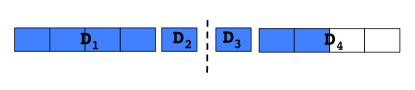
(a) Simulation data as disjoint data.

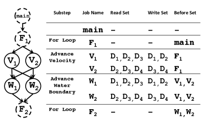
(b) Job graph for one simulation iteration, with each job’s meta-data. Each substep has two jobs that operate over left and right partitions. Dashed jobs spawn new jobs.

Figure 3: Discretized 1D water simulation example under Nimbus abstraction split into two partitions.

3.2 Centralized Controller

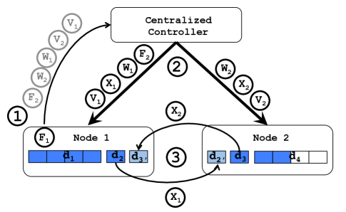
Figure 4: Centralized controller driving 2 nodes for one iteration of discretized 1D water simulation example. Nodes submit jobs to scontroller in phase $1$. Controller instantiates data objects, inserts required data exchanges (X) in between compute jobs and assigns jobs to nodes in phase $2$. Computation and data exchange happen at the nodes in phase $3$.

Centralized controller monitors resources in the cloud and drives a simulation over available resources by issuing commands to the nodes. These commands instantiate data objects, assign computation jobs to nodes, and exchange data values between nodes. The controller distributes simulation state among nodes by instantiating one or more partitions of simulation over each node.

As new jobs are submitted to controller, it builds the job graph from their meta data. The controller uses the job dependencies (before set) and data dependencies (read/write set) to determine what data values to pass to computation jobs – what updates from previous jobs are visible to a job. Based on the existing distribution of data objects, the controller picks a target node for executing a job. If the target node does not have updated data values (e.g. out-dated ghost values), it inserts copy jobs to exchange data between nodes. A runtime before set comprises of all the computation and copy jobs that must run before a job starts executing. It ensures that data accesses are race free, and jobs read correctly updated data. The controller sends a runtime before set, and data instance identifiers to nodes, when issuing a commmand to execute a job. A node executes a job only after all the jobs in its runtime before set complete.

Figure 4 shows one iteration of the simplified water example. A FoorLoop job executes on one of the nodes, and spawns new jobs for the next iteration. The controller issues commands to create data objects $d_{1}$, $d_{2}$ and $d^{\prime}_{3}$ on node $1$, and sends jobs that operate on the left partition to node $1$. Similarly, it issues commands to create data objects $d^{\prime}_{2}$, $d_{3}$ and $d_{4}$, and sends jobs that operate on the right partition to node $2$. After the first set of AdvanceVelocity jobs, ghost values on each node need to be updated from the neighbor. The controller inserts copy jobs to exchange these.

The controller constantly monitors nodes for their health and performance, and redistributes data and computations when a node starts straggling or fails. It regularly checkpoints a simulation by taking a snapshot of the job graph and saving simulation state on persistent memory. Upon failure, it rewinds back to the latest checkpoint and resumes simulation using the saved simulation data. The following section discusses load-balancing and fault-tolerance in more detail.

A design with a centralized controller has two major benefits. First, global knowledge about cloud resources and their performance helps in detecting stragglers and failures. Second, control logic for a simulation does not need to be distributed over multiple nodes – only the centralized controller needs metadata for all jobs. Exchanging job metadata among all nodes to build the job graph at each node induces a lot of overhead in the cloud, due to large network latencies.

4 Implementation

This section covers three main implementation details required to evaluate Nimbus abstraction success in running graphical simulations in presence of stragglers and failures. First, we explain negligible effort in porting current applications into Nimbus. Next, the details of providing load balancing and fault tolerance features are covered. There are a lot of details including controller optimizations that explaining them is out of the scope of this paper.

4.1 Porting Applications

We have ported water and smoke simulation from PhysBAM library into the introduced abstraction, by wrapping existing PhysBAM function calls with Nimbus job abstraction, and adding two loop jobs that spawns the main-loop and the solver-loop with correct job meta data. There are helper functions that help specify read/write/before set, and thus the required changes are small. All in all, water (smoke) simulation required about $2,000$ ($1,300$) additional lines of C++ code to be ported compared to the implemented simulation logic in PhysBAM with over $100,000$ lines of C++ code.

Note that, PhysBAM computations expect to operate over a contiguous data whereas, in our abstraction data is split into disjoin objects. To Eliminate any changes in the code base, we implemented a Translator Layer that translates between the disjoint objects and contiguous data back and forth. The translation happens partially for only the updated objects within the contiguous data. Explaining the details and intricacies of this layer is out of the scope of this paper.

4.2 Load Balancing

Controller tries to distribute computation work uniformly among all nodes by adjusting the simulation region each node is responsible for and assigning jobs accordingly. It carves out the whole simulation region into contiguous regions and ties each region to a node. The target node for job execution would be the node with the region that has the most overlap with the objects in the job’s read/write set. Continuous region assignment eliminates the communication between nodes.

To achieve load balancing, controller reduces the size of the region assigned to a node once it detects the node becomes a straggler. The controller detects stragglers by periodically retrieving performance report from each node. A node is treated as a straggler if the ratio of computation time over total time is over a certain percentage and other nodes are blocking on its ghost cell data transfer.

4.3 Fault Tolerance

Controller periodically creates checkpoints of the simulation state to rewind back from in case of failures. Simulation states are made persistent to disk during checkpointing, and are sharded over different nodes and indexed by a distributed key value store on top of leveldblev .

The states to be checkpointed includes: a snapshot of the job graph, all the parent jobs that submit other jobs to the controller (e.g. For Loop jobs in Figure 3), and all data objects that the parent jobs or the jobs they spawned might access. These saved states are enough for the controller to do a complete rewind back. Upon failure, controller replaces the current job graph with the saved one, assigns the saved parent jobs to nodes for execution, and all data objects that might be possibly accessed are restored. The restored parent jobs will restart the whole simulation from the checkpoint.

5 Evaluation

This section evaluates how Nimbus performs in presence of stragglers and failures. All experiments use a 3D simulation of water pouring into a half full glass gla . We compare Nimbus performance to that of Physbam’s MPI-based distributed implementation. All experiments are run on Amazon EC2; Nimbus controller runs on a $c3.2xlarge$ instance with $15GB$ of RAM and $8$ hyper-threaded cores, while each compute node is a $c3.large$ instance with $3.75GB$ of RAM and $2$ hyper-threaded cores. Unless otherwise stated, all experiments run for $3$ frames and the simulation is $256^{3}$ grid split into $16$ partitions and distributed over $8$ computation nodes. When there are no stragglers or failures, this simulation takes under $15$ minutes.

Figure 5 shows how Nimbus and PhysBAM perform with stragglers. To measure Nimbus’ worst case overhead, we first compare its performance to PhysBAM in an HPC configuration. This is the worst case because it is the environment PhysBAM was designed for – there are no stragglers or failures. Nimbus runs slightly slower in this case. The overhead is primarily round-trip-times between workers and the controller during the linear solve. As Table 1 shows, for every $61ms$ computation period there are more than $1500$ data exchange commands issued from controller to nodes. To compare performance in presence of stragglers, we evaluate Nimbus and Physbam when one of nodes starts straggling $5$ minutes into the simulation. We simulated the straggler by running background processes on one of the nodes (same method as Zaharia et al. [2008]). With this straggler and no load redistribution, the simulation runs $5$ to $6$ times slower . It takes less than $50$ seconds for the controller to detect and adapt to the straggler before converging to a balanced load. PhysBAM cannot adapt and so it goes as slowly as the straggler. However, Nimbus migrates two partitions at the straggler to other two nodes. This way, the simulation runs around $1.5X$ slower, as two nodes run $3$ partitions instead of $2$.

Last we evaluate Nimbus’ fault tolerance mechanisms. In this setup, checkpointing happens every $10$ minutes, and one of the nodes fails after $11$ minutes into the simulation. Figure 6 depicts the iteration progress for a time window. The controller creates a checkpoint after completion of $43^{rd}$ iteration, and one of the nodes fails in the middle of computing $52^{nd}$ iteration. Checkpoint creation overhead is less than $18$ seconds. When the node fails, its in memory state is gone, and controller rewinds back to the last checkpoint, and recomputes the iterations from there. The first iteration after rewinding takes around $153$ seconds which is due to loading aroung $2.4$GB of state from hard disk of remote nodes. Also, iterations take longer after failure because there are less resources available (same as in the straggler case).

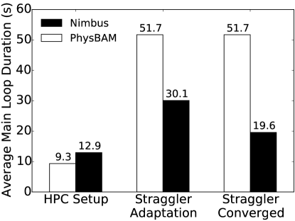
Figure 5: Running a $256^{3}$ water simulation in HPC setting and cloud setting over 8 nodes. Main iteration duration length is measured in case of PhysBAM MPI implementation vs. Nimbus. For the cloud settings the adaptation and converged periods are separated.

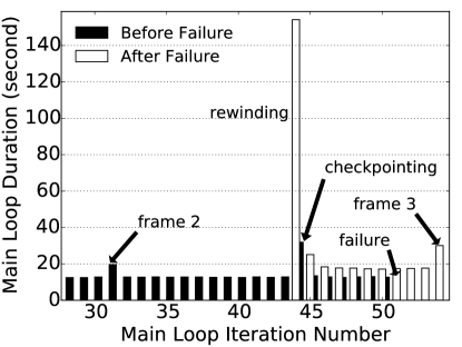
Figure 6: Running a $256^{3}$ water simulation in presence of failure over 8 nodes. Iteration progress is depicted against time. Each ripple shows a checkpoint creation. At each knee one of the nodes has failed and simulation is reverted back by the centralized controller to the last checkpoint.

6 Related Work

Previous work on support for distributing physical simulations, such as Legion Bauer et al. [2012], Charm++ Kale and Krishnan [1993] and adaptive MPI Huang et al. [2004] have focused on supercomputing and high-performance computing environments. Legion provides mechanisms to decouple computations from where they run, but leaves collection and synchronization of runtime information, and actual load-balancing to applications, and does not provide any fault tolerance. Charm++ and adaptive MPI load-balance by migrating chare objects and virtual MPI processes, which do not have any information about geometric locality. Simulation languages such as Liszt DeVito et al. [2011] target portability of code, and use existing mechanisms from the supercomputing domain to parallelize code. Dandelion Rossbach et al. [2013] uses a data flow-engine, similar to Dryad Isard et al. [2007], that is well-suited for parallelism at a coarser granularity.

Existing cloud computing systems such as Map-reduce Dean and Ghemawat [2008] and Spark Zaharia et al. [2010] target highly data parallel computations over key-value stores. Systems such as Pregel Malewicz et al. [2010] and Powergraph Gonzalez et al. [2012] target computations such as scatter and gather over graph data structures. These computations over key-values and graphs have very different access patterns compared to graphical simulations over grids. Nimbus application jobs on the other hand can read and write data at arbitrary locations in their read and write sets. Application job graphs involve complex inter-job and data dependencies in Nimbus.

7 Conclusion and Future Work

Nimbus is a runtime system for running graphical simulation in the cloud. To utilize cloud resources efficiently, Nimbus addresses problems such as stragglers and failures by load-balancing and checkpointing. The key to achieving this is decoupling control flow, computations and data exchanges. With careful design and optimized data structures, the centralized controller does not become a bottleneck at common simulation scales. We have ported a PhysBAM water simulation, an advanced graphical simulation application, to Nimbus with negligible code changes, and proved that Nimbus can adapt to cloud performance problems well.

In future, we plan to explore running more partitions per node to have more flexibility for load balancing, and run even larger simulations. We plan to examine and address scalability issues when running on a large number of nodes. The final objective is to be able to run large simulations on hundreds of elastically provisioned nodes, instead of small and expensive high performance computing clusters.

References

- [1] PhysBAM Water Simulation. http://physbam.stanford.edu/~mlentine/project.html#water.
- [2] InfiniBand. http://www.infinibandta.org/.
- [3] Leveldb. https://github.com/google/leveldb.
- [4] Oscar Aci-Tech Awards. http://www.oscars.org/sci-tech.
- [5] PhysBAM. http://physbam.stanford.edu/.
- [6] protocol buffer. https://github.com/google/protobuf.
- Ananthanarayanan et al. [2010] G. Ananthanarayanan, S. Kandula, A. G. Greenberg, I. Stoica, Y. Lu, B. Saha, and E. Harris. Reining in the outliers in map-reduce clusters using mantri. In OSDI, volume 10, page 24, 2010.
- Bauer et al. [2012] M. Bauer, S. Treichler, E. Slaughter, and A. Aiken. Legion: Expressing locality and independence with logical regions. In High Performance Computing, Networking, Storage and Analysis (SC), 2012 International Conference for, pages 1–11. IEEE, 2012.
- Bridson [2008] R. Bridson. Legion: Expressing locality and independence with logical regions. In Fluid Simulation for Computer Graphics, 2008.
- Corbett et al. [2013] J. C. Corbett, J. Dean, M. Epstein, A. Fikes, C. Frost, J. J. Furman, S. Ghemawat, A. Gubarev, C. Heiser, P. Hochschild, et al. Spanner: Google’s globally distributed database. ACM Transactions on Computer Systems (TOCS), 31(3):8, 2013.
- Dean and Ghemawat [2008] J. Dean and S. Ghemawat. Mapreduce: simplified data processing on large clusters. Communications of the ACM, 51(1):107–113, 2008.
- DeVito et al. [2011] Z. DeVito, N. Joubert, F. Palacios, S. Oakley, M. Medina, M. Barrientos, E. Elsen, F. Ham, A. Aiken, K. Duraisamy, et al. Liszt: a domain specific language for building portable mesh-based pde solvers. In Proceedings of 2011 International Conference for High Performance Computing, Networking, Storage and Analysis, page 9. ACM, 2011.
- Enright et al. [2002] D. Enright, R. Fedkiw, J. Ferziger, and I. Mitchell. A hybrid particle level set method for improved interface capturing. Journal of Computational Physics, 183(1):83–116, 2002.
- Gonzalez et al. [2012] J. E. Gonzalez, Y. Low, H. Gu, D. Bickson, and C. Guestrin. Powergraph: Distributed graph-parallel computation on natural graphs. In OSDI, volume 12, page 2, 2012.
- Harlow et al. [1965] F. H. Harlow, J. E. Welch, et al. Numerical calculation of time-dependent viscous incompressible flow of fluid with free surface. Physics of fluids, 8(12):2182, 1965.
- Huang et al. [2004] C. Huang, O. Lawlor, and L. V. Kale. Adaptive mpi. In Languages and Compilers for Parallel Computing, pages 306–322. Springer, 2004.
- Isard et al. [2007] M. Isard, M. Budiu, Y. Yu, A. Birrell, and D. Fetterly. Dryad: distributed data-parallel programs from sequential building blocks. In ACM SIGOPS Operating Systems Review, volume 41, pages 59–72. ACM, 2007.
- Kale and Krishnan [1993] L. V. Kale and S. Krishnan. CHARM++: a portable concurrent object oriented system based on C++, volume 28. ACM, 1993.
- Malewicz et al. [2010] G. Malewicz, M. H. Austern, A. J. Bik, J. C. Dehnert, I. Horn, N. Leiser, and G. Czajkowski. Pregel: a system for large-scale graph processing. In Proceedings of the 2010 ACM SIGMOD International Conference on Management of data, pages 135–146. ACM, 2010.
- Murray et al. [2013] D. G. Murray, F. McSherry, R. Isaacs, M. Isard, P. Barham, and M. Abadi. Naiad: a timely dataflow system. In Proceedings of the Twenty-Fourth ACM Symposium on Operating Systems Principles, pages 439–455. ACM, 2013.
- Rossbach et al. [2013] C. J. Rossbach, Y. Yu, J. Currey, J.-P. Martin, and D. Fetterly. Dandelion: a compiler and runtime for heterogeneous systems. In Proceedings of the Twenty-Fourth ACM Symposium on Operating Systems Principles, pages 49–68. ACM, 2013.
- Zaharia et al. [2008] M. Zaharia, A. Konwinski, A. D. Joseph, R. H. Katz, and I. Stoica. Improving mapreduce performance in heterogeneous environments. In OSDI, volume 8, page 7, 2008.
- Zaharia et al. [2010] M. Zaharia, M. Chowdhury, M. J. Franklin, S. Shenker, and I. Stoica. Spark: cluster computing with working sets. In Proceedings of the 2nd USENIX conference on Hot topics in cloud computing, pages 10–10, 2010.