Abstract

We present revised measurements of the static electric dipole polarizabilities of K, Rb, and Cs based on atom interferometer experiments presented in [Phys. Rev. A 2015, 92, 052513] but now re-analyzed with new calibrations for the magnitude and geometry of the applied electric field gradient. The resulting polarizability values did not change, but the uncertainties were significantly reduced. Then we interpret several measurements of alkali metal atomic polarizabilities in terms of atomic oscillator strengths $f_{ik}$, Einstein coefficients $A_{ik}$, state lifetimes $\tau_{k}$, transition dipole matrix elements $D_{ik}$, line strengths $S_{ik}$, and van der Waals $C_{6}$ coefficients. Finally, we combine atom interferometer measurements of polarizabilities with independent measurements of lifetimes and $C_{6}$ values in order to quantify the residual contribution to polarizability due to all atomic transitions other than the principal $ns$-$np_{J}$ transitions for alkali metal atoms.

x 10.3390/—— xx Academic Editor: name Received: date; Accepted: date; Published: date Analysis of polarizability measurements made with atom interferometry Maxwell D. Gregoire ¹, Nathan Brooks ¹, Raisa Trubko², and Alexander D. Cronin ^1,2* Maxwell D. Gregoire, Nathan Brooks, Raisa Trubko, and Alexander D. Cronin Correspondence: cronin@physics.arizona.edu; Tel.: 520-465-8459

1 Introduction

Atomic and molecular interferometry Berman (1997); Cronin et al. (2009) has become a precise method for measuring atomic properties such as static polarizabilities Gregoire et al. (2015); Ekstrom et al. (1995); Miffre et al. (2006); Berninger et al. (2007); Holmgren et al. (2010), van der Waals interactions Perreault and Cronin (2005); Lepoutre et al. (2009, 2011), and tune-out wavelengths Holmgren et al. (2012); Leonard et al. (2015). Calculating these atomic and molecular properties ab initio is challenging because it requires modeling of quantum many-body systems with relativistic corrections. For example, different methods for calculating polarizabilities yield results that vary by as much as 10% for Cs Mitroy et al. (2010); Tang et al. (2009); Sahoo (2007); Hamonou and Hibbert (2007); Deiglmayr et al. (2008); Johnson et al. (2008); Reinsch and Meyer (1976); Tang (1976); Maeder and Kutzelnigg (1979); Christiansen and Pitzer (1982); Fuentealba (1982); Müller et al. (1984); Kundu et al. (1986); Kello et al. (1993); Fuentealba and Reyes (1993); Marinescu et al. (1994); Dolg (1996); Patil and Tang (1997); Lim et al. (1999); Safronova et al. (1999); Derevianko et al. (1999); Magnier and Aubert-Frécon (2002); Mitroy and Bromley (2003); Safronova and Clark (2004); Lim et al. (2005); Arora et al. (2007); Iskrenova-Tchoukova et al. (2007); Safronova and Safronova (2008, 2011). For molecules the challenges are even greater. Furthermore, determining the uncertainty for an ab initio calculation can be difficult. Polarizability measurements made with matter wave interferometry, therefore, have been used to assess which calculation methods are most valid. Testing these calculations is important because similar methods are used to predict atomic scattering cross sections, Feshbach resonances, photoassociation rates, atom-surface van-der Waals $C_{3}$ coefficients, atomic parity-violating amplitudes, and atomic clock shifts due to thermal radiation or collisions.

In this manuscript, we first present revised uncertainties on our most recent K, Rb, and Cs static polarizability measurements Gregoire et al. (2015) in Section 2. We then show how to use polarizability measurements for alkali metal atoms Ekstrom et al. (1995); Miffre et al. (2006); Holmgren et al. (2010); Gregoire et al. (2015) as input for semi-empirical calculations of atomic properties such as oscillator strengths, Einstein $A$ coefficients, state lifetimes, transition matrix elements, and line strengths, as we discuss in Section 3.1. We use polarizability measurements to predict van der Waals $C_{6}$ coefficients in Section 3.2. To support this analysis, throughout Section 3 we use theoretical values for so-called residual polarizabilities of alkali metal atoms, i.e. the contributions to polarizabilities that come higher-energy excitations associated with the inner-shell (core) electrons and highly-excited states of the valence electrons. The idea-chart in Fig. 1 shows connections between the residual polarizability ($\alpha_{r}$) and several quantities related via Eqns. (1)-(17) that we use to interpret polarizabilities.

Then in Section 4 we demonstrate an all-experimental method for measuring residual polarizabilities. We do this by using polarizability measurements in combination with independent measurements of lifetimes and van der Waals $C_{6}$ coefficients. This serves as a cross-check for some assumptions used in Section 3 that are also used for analysis of atomic parity violation and atomic clocks. Section 4 highlights how atom interferometry measurements shown in Table 1 are sufficiently precise to directly measure the static residual polarizability, $\alpha_{r}(0)$, for each of the alkali-metal atoms, Li, Na, K, Rb, and Cs.

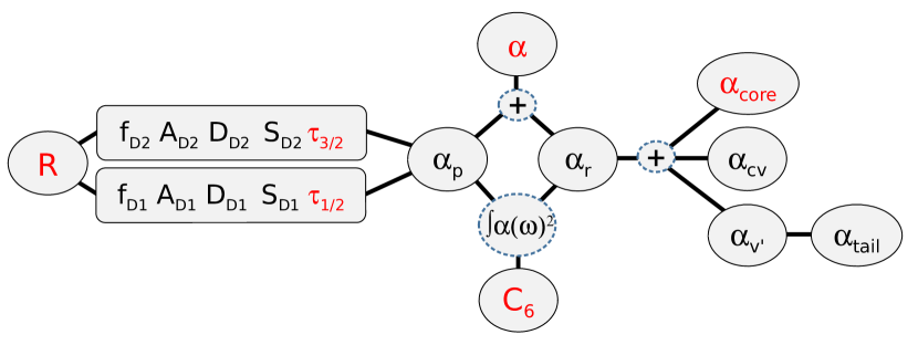
Figure 1: An idea chart showing connections between various quantities defined in Equations (1)-(17) that we relate to static polarizability $\alpha(0)$ for alkali metal atoms. Quantities in red have been directly measured.

2 Revised uncertainties on recent polarizability measurements

We reduced the uncertainties in our most recent K, Rb, and Cs static polarizability measurements Gregoire et al. (2015) to 0.11% by reducing the total systematic uncertainty from 0.15% to 0.10%. In our experiment, we used cylindrical electrodes, indicated in red in Fig. 2, to induce phase shifts in our atom interferometer that are proportional to $\alpha(0)V^{2}$, the atoms’ static polarizabilities times the square of the voltage difference between the electrodes. Fig. 3a shows an example of how the induced phase shift changes as we move the electrodes laterally with respect to the beamline.

We reduced the systematic uncertainty in our measurements from 0.15% to 0.12% by calibrating the voltage supplies connected to the electrodes to 36 ppm using a Vitrek 4700 high-accuracy voltmeter. Each electrode is held at its respective positive or negative voltage with respect to ground by its own power supply. We concluded that when we instructed the power supplies to output $\pm 6$ kV, both power supplies were actually supplying $\pm 6.0026(2)$ kV. Our results agreed with less-accurate calibration measurements of $\pm 6.003(3)$ we made earlier using a Fluke 287 multimeter and a Fluke 80k-40 high-voltage probe. At normal operating temperatures, our calibration measurements were completely reproducible to within the resolution of the Vitrek 4700.

The strength of the electric field gradient, and therefore the magnitude of the induced phase shift, also depends on the distance between the electrodes. In the past, we measured that distance to be 1999.9(5) $\mu$m by sweeping the electrodes across the beamline and measuring the lateral positions at which the electrodes eclipsed the beam (see an example of these data in Fig. 3b). We found that scatter in our measurements was explained by misalignment of the collimating slits and detector. After correcting for this source of error, we measured the distance between electrodes to be 1999.7(2) $\mu$m, which further reduced our total systematic uncertainty from 0.12% to 0.10%. Our measurements did not change as a function of maximum atom flux, electrodes translation motor speed, atom beam $y$ position or vertical collimation, atom beam velocity, or atomic species.

By themselves, the new values we measured for the electrodes’ voltages and the distance between the electrodes changed our reported polarizabilities by +140 ppm and -140 ppm, respectively. Therefore, the polarizability values that we report are the same as those in Gregoire et al. (2015) but with smaller uncertainties. It is also worth noting that either of the $\pm 140$ ppm changes, by itself, would still not have been statistically significant. These reduced total uncertainties are shown alongside the previously-reported values in Table 1.

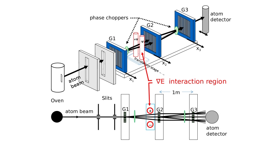
Figure 2: Diagram of the atom interferometer we used to measure the static polarizabilities of K, Rb, and Cs Gregoire et al. (2015). A pair of cylindrical, oppositely-charged electrodes, indicated in red, induce phase shifts that depend on atoms’ polarizabilities and the gradient of the produced electric field.

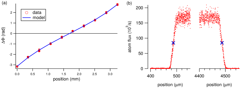
Figure 3: (a): Induced phase shift in the interferometer vs the lateral position of the electrodes with respect to the beam. (b): Observed atom beam flux as a function of the electrodes’ lateral position. We use these data to determine the distance between the electrodes.

3 Analysis of atom interferometry polarizability measurements

Table 1 lists polarizability measurements made with atom interferometry. For Li, Na, K, Rb, and Cs, atom interferometry has provided the best available measurements. Polarizability measurements made using other methods are reviewed in Amini and Gould (2003); Mitroy et al. (2010); Schwerdtfeger (2006, ); Gould and Miller (2005); Haynes (2014).

Table 1: Measurements of static polarizabilities $\alpha(0)$ made using atom or molecule interferometry. References Ekstrom et al. (1995); Miffre et al. (2006) used a septum electrode and references Berninger et al. (2007); Holmgren et al. (2010); Gregoire et al. (2015) used electric field gradients to shift the phase of matter wave interference fringes. Results are presented both in ų and atomic units (au). Values we use for analysis in this paper are in bold.

Atom or	Polarizability		Reference	Uncertainty
molecule	(Å3)	(au)
Li	24.33(16)	164.2(11)	Miffre et al. (2006)	0.66%
Na	24.11(8)	162.7(5)	Ekstrom et al. (1995)	0.35%
Na	24.11(18)	162.7(12)	Holmgren et al. (2010)	0.75%
K	43.06(21)	290.6(14)	Holmgren et al. (2010)	0.49%
K	42.93(7)	289.7(5)	Gregoire et al. (2015)	0.16%
K	42.93(5)	289.7(3)	this work	0.11%
Rb	47.24(21)	318.8(14)	Holmgren et al. (2010)	0.44%
Rb	47.39(8)	319.8(5)	Gregoire et al. (2015)	0.17%
Rb	47.39(5)	319.8(3)	this work	0.11%
Cs	59.39(9)	400.8(6)	Gregoire et al. (2015)	0.15%
Cs	59.39(6)	400.8(4)	this work	0.11%
C60	88.9(52)	600(35)	Berninger et al. (2007)	5.9%
C70	108.5(65)	732(44)	Berninger et al. (2007)	6.5%

The original references Ekstrom et al. (1995); Holmgren et al. (2010); Gregoire et al. (2015) show how the polarizability measurements in Table 1 compare to theoretical predictions Mitroy et al. (2010); Reinsch and Meyer (1976); Tang (1976); Maeder and Kutzelnigg (1979); Christiansen and Pitzer (1982); Fuentealba (1982); Müller et al. (1984); Kundu et al. (1986); Kello et al. (1993); Fuentealba and Reyes (1993); Marinescu et al. (1994); Dolg (1996); Patil and Tang (1997); Lim et al. (1999); Safronova et al. (1999); Derevianko et al. (1999); Magnier and Aubert-Frécon (2002); Mitroy and Bromley (2003); Safronova and Clark (2004); Lim et al. (2005); Arora et al. (2007); Iskrenova-Tchoukova et al. (2007); Safronova and Safronova (2008, 2011). In this article, we devote our attention to interpreting the atomic polarizability measurements in Table 1 in a systematic and tutorial manner. In the rest of Section 3 we show how to use these polarizability measurements to predit other atomic properties such as oscillator strengths, lifetimes, matrix elements, line strengths, and van der Waals $C_{6}$ coefficients, following procedures described earlier by Derevianko and Porsev Derevianko and Porsev (2002), Amini and Gould Amini and Gould (2003), and Mitroy, Safronova, and Clark Mitroy et al. (2010) among others. Then, in Section 4, we use the polarizabilities in Table 1 to provide experimental constraints on the residual polarizabilities, $\alpha_{r}$, for each of the alklai atoms.

3.1 Reporting oscillator strengths, lifetimes, matrix elements, and line strengths from static polarizabilities

The dynamic polarizability, $\alpha(\omega)$, of an atom in state $|i\rangle$ can be written as a sum over electric-dipole transition matrix elements $\langle k|e\vec{r}|i\rangle$, Einstein coefficients $A_{ik}$, oscillator strengths $f_{ik}$, or line strengths $S_{ik}$ as

$$\alpha(\omega) =\frac{e^{2}}{m}\sum_{k\neq i}\frac{f_{ik}}{\omega_{ik}^{2}-\omega^{2}}$$ (1)

$$\alpha(\omega) =2\pi\epsilon_{0}c^{3}\sum_{k\neq i}\frac{A_{ki}\omega_{ik}^{-2}}{\omega_{ik}^{2}-\omega^{2}}\frac{g_{k}}{g_{i}}$$ (2)

$$\alpha(\omega) =\frac{2}{3\hbar}\sum_{k\neq i}\frac{|\langle k|e\vec{r}|i\rangle|^{2}\omega_{ik}}{\omega_{ik}^{2}-\omega^{2}}$$ (3)

$$\alpha(\omega) =\frac{1}{3\hbar}\sum_{k\neq i}\frac{S_{ik}\omega_{ik}}{\omega_{ik}^{2}-\omega^{2}}$$ (4)

where $e$ and $m$ are the charge and mass of an electron, $\omega_{ik}=(E_{k}-E_{i})/\hbar$ are resonant frequencies for excitation from state $|i\rangle$ to state $|k\rangle$, and $g_{k}=2J_{k}+1$ is the degeneracy of state $|k\rangle$. The squares of electric dipole transition matrix elements $|\langle k|e\vec{r}|i\rangle|^{2}$, or equivalently $3|\langle k|e\vec{x}|i\rangle|^{2}$, are related to the reduced dipole matrix elements (denoted with double bars) by $|\langle k\|e\vec{r}\|i\rangle|^{2}=|D_{ik}|^{2}=\sum_{m_{k},m_{i}}|\langle k|e\vec{r}|i\rangle|^{2}=|\langle k|e\vec{r}|i\rangle|^{2}g_{i}$ using the Wigner-Eckart theorem. For ground state alkali atoms, line strength $S_{ik}=|D_{ik}|^{2}$.

The expressions for polarizability $\alpha(0)$ in Eqs. (1) - (4) each have dimensions of $4\pi\epsilon_{0}$ times volume, as expected from the definitions $\vec{p}=\alpha\vec{E}$ and $U=-\frac{1}{2}\alpha|\vec{E}|^{2}$, where $\vec{p}$ is the induced dipole moment and $U$ is the energy shift (Stark shift) of an atom in an electric field $\vec{E}$. When polarizability is reported in units of volume (typically ų or $10^{-24}$ cm³) it is implied that one can multiply by $4\pi\epsilon_{0}$ to get polarizability in SI units. The atomic unit (au) of polarizability, $e^{2}a_{0}^{2}/E_{h}$, is equivalent to $a_{0}^{3}\times 4\pi\epsilon_{0}$, where $a_{0}$ is the Bohr radius, and $E_{h}$ is a Hartree. Since $(4\pi\epsilon_{0})=1$ in au, polarizability is naturally expressed in atomic units of volume of $a_{0}^{3}$ (and for reference $a_{0}^{3}=0.148185$ ų).

Since the principal D1 and D2 transitions of alkali metal atoms (denoting the $ns$-$np_{1/2}$ and $ns$-$np_{3/2}$ transitions respectively, where $n$=6 for Cs, $n$=5 for Rb, $n$=4 for K, $n$=3 for Na, and $n$=2 for Li), account for over 95% of those atoms’ static polarizabilities Derevianko et al. (1999), it is customary to decompose polarizability as

$$\alpha(\omega)=\alpha_{p}(\omega)+\alpha_{r}(\omega)$$ (5)

where $\alpha_{p}(\omega)$ represents the contribution from the principal transitions and $\alpha_{r}(\omega)$ is the residual polarizability due to all other excitations. The residual polarizability itself can be further decomposed as

$$\alpha_{r}(\omega)=\alpha_{v^{\prime}}(\omega)+\alpha_{\mathrm{core}}(\omega)+\alpha_{cv}(\omega)$$ (6)

where $\alpha_{v^{\prime}}$ is due to higher $ns_{1/2}-n^{\prime}p_{J}$ excitations of the valence electron with $n^{\prime}>n$, $\alpha_{\mathrm{core}}$ is the polariability due to the core electrons, and $\alpha_{cv}$ is due to correlations between core and valence electrons. Sometimes the notation $\alpha_{\mathrm{tail}}$ is used to denote a subset of $\alpha_{v^{\prime}}$ with $n^{\prime}>(n+3)$ Safronova et al. (2006), or $n^{\prime}>(n+5)$ Safronova et al. (1999), or an even higher cutoff such as $n^{\prime}>26$ Safronova and Safronova (2008).

Using the decomposition in Eqn. (5) we can rewrite Eqs. (1)-(4) for static ($\omega=0$) polarizabilities:

$$\alpha(0) =\frac{e^{2}}{m}\left[\frac{f_{D1}}{\omega_{D1}^{2}}+\frac{f_{D2}}{\omega_{D2}^{2}}\right]+\alpha_{r}(0)$$ (7)

$$\alpha(0) =2\pi\epsilon_{0}c^{3}\left[\frac{\tau_{1/2}^{-1}}{\omega_{D1}^{4}}+2\frac{\tau_{3/2}^{-1}}{\omega_{D2}^{4}}\right]+\alpha_{r}(0)$$ (8)

$$\alpha(0) =\frac{1}{3\hbar}\left[\frac{|D_{D1}|^{2}}{\omega_{D1}}+\frac{|D_{D2}|^{2}}{\omega_{D2}}\right]+\alpha_{r}(0)$$ (9)

$$\alpha(0) =\frac{1}{3\hbar}\left[\frac{S_{D1}}{\omega_{D1}}+\frac{S_{D2}}{\omega_{D2}}\right]+\alpha_{r}(0)$$ (10)

Eqn. (8) is written in terms of lifetimes $\tau_{k}^{-1}=\sum_{i}A_{ki}$, rather than Einstein $A$ coefficients because alkali metal atom $np_{J}$ states decay with a branching ratio of 100% to their respective ground $ns_{1/2}$ states. To support our analysis of polarizabilites here in Section 3 we use theoretically caclulated values of residual static polarizabilities $\alpha_{r}(0)$ = 2.04(69) au for Li, $\alpha_{r}(0)$ = 1.86(12) au for Na, $\alpha_{r}(0)$ = 6.26(33) au for K, $\alpha_{r}(0)$ = 10.54(60) au for Rb, all from Savronova et al.Safronova et al. (2006), and $\alpha_{r}(0)$ = 16.74(11) au for Cs from Derevianko et al.Derevianko and Porsev (2002). Table 6 in Appendix A lists these and several other published values for $\alpha_{\mathrm{core}}(0)$, $\alpha_{v^{\prime}}(0)$, $\alpha_{cv}(0)$ and $\alpha_{r}(0)$.

Since $\omega_{D1}$ and $\omega_{D2}$ are well known NIST , we can further use Eqs. (7)-(10) to derive expressions for $|D_{ik}|^{2}$, $\tau_{k}$, and $f_{ik}$ in terms of $\alpha(0)$, $\alpha_{r}(0)$, and a ratio of line strengths $R$:

$$f_{D1} =\frac{\left[\alpha(0)-\alpha_{r}(0)\right]}{\left(\frac{e^{2}}{m\omega_{D1}^{2}}\right)}\left(\frac{1}{1+R\frac{\omega_{D1}}{\omega_{D2}}}\right)$$ (11)

$$f_{D2} =\frac{\left[\alpha(0)-\alpha_{r}(0)\right]}{\left(\frac{e^{2}}{m\omega_{D1}^{2}}\right)}\left(\frac{R}{\frac{\omega_{D2}}{\omega_{D1}}+R}\right)$$ (12)

$$\tau_{1/2} =\frac{2\pi\epsilon_{0}c^{3}\omega_{D1}^{-3}}{\left[\alpha(0)-\alpha_{r}(0)\right]}\left(\frac{1}{\omega_{D1}}+\frac{R}{\omega_{D2}}\right)$$ (13)

$$\tau_{3/2} =\frac{2\pi\epsilon_{0}c^{3}\omega_{D2}^{-3}}{\left[\alpha(0)-\alpha_{r}(0)\right]}\left(\frac{2}{R\omega_{D1}}+\frac{2}{\omega_{D2}}\right)$$ (14)

$$|D_{D1}|^{2} =S_{D1}=\left[\alpha(0)-\alpha_{r}(0)\right]\left(\frac{3\hbar}{\frac{1}{\omega_{D1}}+\frac{R}{\omega_{D2}}}\right)$$ (15)

$$|D_{D2}|^{2} =S_{D2}=\left[\alpha(0)-\alpha_{r}(0)\right]\left(\frac{3\hbar}{\frac{1}{R\omega_{D1}}+\frac{1}{\omega_{D2}}}\right)$$ (16)

where $R$ is defined as

$$R\equiv\frac{S_{D2}}{S_{D1}}=\frac{|D_{D2}|^{2}}{|D_{D1}|^{2}}=\frac{f_{D2}}{f_{D1}}\frac{\omega_{D1}}{\omega_{D2}}=2\frac{\tau_{1/2}}{\tau_{3/2}}\left(\frac{\omega_{D1}}{\omega_{D2}}\right)^{3}$$ (17)

To support our analysis of polarizabilities, we will use $R$= 2.0000 for Li inferred from Johnson et al. (2008), $R$=1.9994(37) for Na Volz and Schmoranzer (1996), $R$=1.9976(13) for K Trubko (2016), $R$=1.99219(3) for Rb Leonard et al. (2015) , and $R$= 1.9809(9) for Cs Rafac and Tanner (1998). It is noteworthy that references Holmgren et al. (2012); Leonard et al. (2015); Trubko (2016) determined $R$ experimentally using atom interferometry measurements of tune-out wavelengths.

Table 2: Atomic properties inferred from atom interferometry measurements Ekstrom et al. (1995); Miffre et al. (2006); Gregoire et al. (2015). Reduced matrix elements $D_{D1}=\langle np_{1/2}\|r\|ns_{1/2}\rangle$ and $D_{D2}=\langle np_{3/2}\|r\|ns_{1/2}\rangle$, lifetimes $\tau_{np1/2}$ and $\tau_{np3/2}$, oscillator strengths $f$, and line strengths $S$ shown here are inferred from measurements of polarizabilities, $\alpha(0)$ shown in Table 1 using Eqns (11) - (16). Subscripts D1 and D2 refer to the $ns$-$np_{1/2}$ and $ns$-$np_{3/2}$ transitions respectively, where $n$=6 for Cs, $n$=5 for Rb, $n$=4 for K, $n$=3 for Na and $n$=2 for Li. Uncertainty budget components $\delta_{\alpha}$, $\delta_{R}$, and $\delta_{\alpha_{r}}$ come from the uncertainties in $\alpha(0)$ Ekstrom et al. (1995); Miffre et al. (2006); Gregoire et al. (2015) (see Table 1), $R$ Johnson et al. (2008); Volz and Schmoranzer (1996); Trubko (2016); Leonard et al. (2015); Rafac and Tanner (1998), and $\alpha_{r}(0)$ Safronova et al. (2006); Derevianko and Porsev (2002) (see Table 6). The resulting uncertainties for $D_{D1}$, $D_{D2}$, $\tau_{np1/2}$, $\tau_{np3/2}$, $f_{D1}$, $f_{D2}$, $S_{D1}$, and $S_{D2}$ are reported presuming possible errors $\delta_{\alpha}$, $\delta_{R}$, and $\delta_{\alpha_{r}}$ are uncorrelated. The symbol (-) indicates an uncertainty $<1$ in the least significant digit.

atom	$D_{D1}$ (au)	$\delta_{\alpha}$	$\delta_{R}$	$\delta_{\alpha_{r}}$		$D_{D2}$ (au)	$\delta_{\alpha}$	$\delta_{R}$	$\delta_{\alpha_{r}}$
Li	3.318(13)	(11)	(-)	(7)		4.693(19)	(16)	(-)	(10)
Na	3.527(6)	(6)	(2)	(1)		4.987(8)	(8)	(2)	(2)
K	4.101(4)	(3)	(1)	(2)		5.800(5)	(4)	(1)	(3)
Rb	4.239(5)	(3)	(-)	(4)		5.989(7)	(4)	(-)	(6)
Cs	4.508(3)	(3)	(1)	(1)		6.345(4)	(4)	(-)	(1)
atom	$\tau_{1/2}$ (ns)	$\delta_{\alpha}$	$\delta_{R}$	$\delta_{\alpha_{r}}$		$\tau_{3/2}$ (ns)	$\delta_{\alpha}$	$\delta_{R}$	$\delta_{\alpha_{r}}$
Li	27.08(21)	(18)	(-)	(11)		27.08(21)	(18)	(-)	(11)
Na	16.28(6)	(5)	(2)	(3)		16.24(5)	(5)	(1)	(1)
K	26.80(4)	(3)	(1)	(3)		26.45(4)	(3)	(1)	(3)
Rb	27.60(6)	(3)	(-)	(5)		26.14(6)	(3)	(-)	(5)
Cs	34.77(5)	(5)	(1)	(1)		30.37(5)	(4)	(1)	(-)
atom	$f_{D1}$	$\delta_{\alpha}$	$\delta_{R}$	$\delta_{\alpha_{r}}$		$f_{D2}$	$\delta_{\alpha}$	$\delta_{R}$	$\delta_{\alpha_{r}}$
Li	0.2492(20)	(17)	(-)	(11)		0.4985(39)	(33)	(-)	(39)
Na	0.3203(12)	(11)	(4)	(2)		0.6410(23)	(22)	(4)	(5)
K	0.3317(6)	(4)	(1)	(4)		0.6665(11)	(8)	(1)	(7)
Rb	0.3438(8)	(4)	(-)	(7)		0.6982(17)	(9)	(-)	(14)
Cs	0.3450(5)	(5)	(1)	(1)		0.7174(10)	(10)	(1)	(2)
atom	$S_{D1}$ (au)	$\delta_{\alpha}$	$\delta_{R}$	$\delta_{\alpha_{r}}$		$S_{D2}$ (au)	$\delta_{\alpha}$	$\delta_{R}$	$\delta_{\alpha_{r}}$
Li	11.01(9)	(8)	(-)	(5)		22.02(17)	(15)	(-)	(9)
Na	12.44(5)	(4)	(2)	(1)		24.87(8)	(8)	(2)	(2)
K	16.82(3)	(2)	(1)	(2)		33.64(6)	(4)	(1)	(4)
Rb	17.97(4)	(3)	(-)	(3)		35.87(8)	(4)	(-)	(7)
Cs	20.32(3)	(3)	(1)	(1)		40.26(5)	(5)	(1)	(1)

Table 2 shows principal transition matrix elements, lifetimes, line strengths, and oscillator strengths inferred from polarizability measurements using Eqns. (11)-(17). Our inferred lifetimes for K, Rb, and Cs are based on $\alpha(0)$ measurements with 0.11% uncertainty, yet our derived lifetimes have slightly larger uncertainty. In the case of Li, Na, K and Rb, this is because roughly half of the total uncertainty comes from uncertainty in $\alpha_{r}(0)$, whereas for Cs the uncertainties in $\tau$ are dominated by contributions from uncertainty in $\alpha(0)$. Because there have been many high precision measurements of alkali metal principal transition lifetimes, it is useful to compare our derived lifetimes to those measurements. Our derived K and Rb lifetimes agree well with and have comparable uncertainty to those measured by Volz et al.Volz and Schmoranzer (1996), Wang et al.Wang et al. (1997a, b), and Simsarian et al.Simsarian et al. (1998). Because the $\alpha(0)$ measurements used to derive the Li and Na lifetimes in Table 2 are less precise, our inferred Na lifetimes have about twice the uncertainty (about 0.4%) of measurements by Volz et al.Volz and Schmoranzer (1996), and our inferred Li lifetimes have much greater uncertainty than measurements by Volz et al.Volz and Schmoranzer (1996) and McAlexander et al.McAlexander et al. (1996).

For Cs, the lifetimes we report in Table 2 for this work have an uncertainty of less than 0.15%, which is slightly smaller than the uncertainty of four previous high-precision determinations of the Cs $6p_{J}$ state lifetimes Rafac et al. (1994); Young et al. (1994); Rafac et al. (1999); Derevianko and Porsev (2002). Table 3 and Fig. 4 show how our lifetime results are consistent with Young et al. (1994); Derevianko and Porsev (2002) but differ from lifetimes reported in Rafac et al. (1994, 1999). Our results deviate by 1.5$\sigma$ from $\tau_{1/2}$ found in Rafac et al. (1994) and by 3$\sigma$ from $\tau_{1/2}$ in Rafac et al. (1999), where $\sigma$ for the deviations here refers to the combined uncertainty (added in quadrature) for the experiments. Comparing the sum of line strengths ($S_{D1}+S_{D2}$), a quantity that is mostly independent of $R$, provides a similar conclusion: our results are consistent with Young et al. (1994) and Derevianko and Porsev (2002) but differ by two and three $\sigma$ from Rafac et al. (1994) and Rafac et al. (1999).

Because the two recent measurements of $\alpha_{\textrm{Cs}}(0)$ by Gregoire et al.Gregoire et al. (2015) and Amini and Gould Amini and Gould (2003) were made using very different methods, we combine these measurements using a weighted average in order to report a value for $\tau_{6p_{1/2},\mathrm{Cs}}$ with even smaller (0.03 ns) uncertainty in Table 3. We note that, due to the uncertainty in $R$ and $\alpha_{r}(0)$, the uncertainty in $\tau_{6p_{1/2},\mathrm{Cs}}$ would still be 0.01 ns even if the polarizability measurements had no uncertainty.

The Cs $|D_{D1}|$ value calculated ab initio by Porsev et al. (2010) is also consistent with our results for $|D_{D1}|$. Since our results come from independent measurements of $\alpha(0)$ and $R$, combined with theoretical values for $\alpha_{r}(0)$ , the agreement between our result for $|D_{D1}|$ with the that of Derevianko and Porsev Derevianko and Porsev (2002); Porsev et al. (2010) adds confidence to their analysis of atomic parity violation Porsev et al. (2009, 2010).

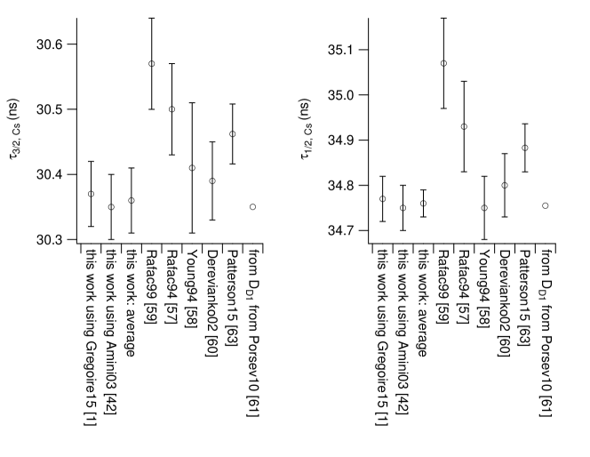
Figure 4: Comparisons of Cs principal transition lifetimes inferred from polarizability measurements Amini and Gould (2003); Gregoire et al. (2015) and theoretical $\alpha_{r,\textrm{Cs}}(0)$ Derevianko and Porsev (2002), direct measurements Rafac et al. (1999, 1994); Young et al. (1994); Derevianko and Porsev (2002), and a combination of Porsev et al.’s calculated $|D_{D1}|$ Porsev et al. (2010) and $R$ Rafac and Tanner (1998).

Table 3: Cesium $6p_{J}$ lifetimes ($\tau_{J}$) from several references, tabulated here for comparison. The $\tau_{2/1}$ and $\tau_{3/2}$ values that we report using $\alpha(0)$ measured by atom interferometry et al.Gregoire et al. (2015) (combined with values of $\alpha_{r}(0)$ Porsev et al. (2010) and $R$ Rafac and Tanner (1998)) are reproduced from Table 2. Similar comparisons appear in Table II of Amini and Gould (2003) and Table I of Patterson et al. (2015).

$\tau_{1/2}$ (ns)	$\tau_{3/2}$ (ns)	Method and Reference(s)
34.77(5)	30.37(5)	this work using $\alpha(0)$ from atom interferometry Gregoire et al. (2015)
34.75(5)	30.35(5)	this approach using $\alpha(0)$ from Amini and Gould (2003)
34.76(3)	30.36(3)	this approach using $\alpha(0)$ from both Gregoire et al. (2015) and Amini and Gould (2003)
35.07(10)	30.57(7)	Rafac et al. (1999) Rafac 1999
34.93(10)	30.50(7)	Rafac et al. (1994) Rafac 1994
34.75(7)	30.41(10)	Young et al. (1994) Young 1994
34.80(7)	30.39(6)	Derevianko and Porsev (2002) Derevianko 2002
34.883(53)	30.462(46)	$\tau_{3/2}$ from Patterson et al. (2015), combined with $R$ Rafac and Tanner (1998) to infer $\tau_{1/2}$
34.755	30.3502	from $D_{D1}$ calculation by Porsev et al. (2010), combined with $R$ Rafac and Tanner (1998) to infer $\tau_{3/2}$

3.2 Deriving van der Waals coefficients from polarizabilities

Since polarizability determines the strengths of van der Waals (vdW) potentials, we can also use measurements of $\alpha(0)$ to improve predictions for atom-atom interactions. Two ground-state atoms have a van der Waals interaction potential

$$U=-\frac{C_{6}}{r^{6}}-\frac{C_{8}}{r^{8}}-\frac{C_{10}}{r^{10}}+...$$ (18)

where $r$ is the inter-nuclear distance and $C_{6}$, $C_{8}$, and $C_{10}$ are dispersion coefficients that can be predicted based on $\alpha(0)$ measurements. For long-range interactions in the absence of retardation (i.e. for $a_{0}\ll r\ll c/\omega_{D2}$), the $C_{6}$ term is most important. The $C_{6}$ coefficient for homo-nuclear atom-atom vdW interactions depends on dynamic polarizability as

$$C_{6}=\frac{3\hbar}{\pi}\int_{0}^{\infty}\left[\alpha(i\omega)\right]^{2}d\omega$$ (19)

Even though $\hbar=1$ in au, we write $\hbar$ explicitly in Eqn. (19) to emphasize that the dimensions of $C_{6}$ are energy $\times$ length⁶.

The London result of $C_{6}=(3/4)\hbar\omega_{0}\alpha(0)^{2}$ can be found from Eqn. (19) by using Eqn. (1) for $\alpha(i\omega)$ with a single term in the sum to represent an atom as a single oscillator of frequency $\omega_{0}$ with static polarizability $\alpha(0)$. However, calculating $C_{6}$ gets more difficult for atoms with multiple oscillator strengths. In light of this complexity, we instead use the decomposition in Eqn. (5) to express $C_{6}$ as

$$C_{6} =\frac{3\hbar}{\pi}\int_{0}^{\infty}\left[\alpha_{p}(i\omega)+\alpha_{r}(i\omega)\right]^{2}d\omega$$

$$=\frac{3\hbar}{\pi}\int_{0}^{\infty}\left[\alpha_{p}(i\omega)\right]^{2}d\omega+\frac{6\hbar}{\pi}\int_{0}^{\infty}\alpha_{p}(i\omega)\alpha_{r}(i\omega)d\omega+\frac{3\hbar}{\pi}\int_{0}^{\infty}\left[\alpha_{r}(i\omega)\right]^{2}d\omega$$ (20)

Because of the cross term, the integration over frequency, and the way $\alpha(i\omega)$ remains relatively constant until ultraviolet frequencies, $\alpha_{r}$ is significantly more important for $C_{6}$ than for $\alpha(0)$. Contributions from $\alpha_{r}$ account for 15% of $C_{6}$ whereas $\alpha_{r}$ contributes only 4% to $\alpha(0)$ for Cs, as pointed out by Derevianko et al.Derevianko et al. (1999).

The fact that $C_{6}$ and $\alpha(0)$ depend on $\alpha_{r}$ in different ways [compare Eqns. (5) and (20)] suggests that it is possible to determine $\alpha_{r}(0)$ based on independent measurements of $C_{6}$ and $\alpha(0)$. We will explore this in Section 4. First, we want to demonstrate how to use experimental $\alpha(0)$ measurements and theoretical $\alpha_{r}(i\omega)$ spectra to improve predictions of $C_{6}$ coefficients. For this we begin by factoring $\alpha_{p}(0)$ out of the $\alpha_{p}(i\omega)$ term in the integrand of Eqn. (20) to get

$$C_{6}=\frac{3\hbar}{\pi}\int_{0}^{\infty}\left[\alpha_{p}(0)\frac{\alpha_{p}(i\omega)}{\alpha_{p}(0)}+\alpha_{r}(i\omega)\right]^{2}d\omega$$ (21)

where the spectral shape function

$$\frac{\alpha_{p}(i\omega)}{\alpha_{p}(0)}=\frac{\frac{1}{\omega_{D1}^{2}+\omega^{2}}+\frac{R\frac{\omega_{D1}}{\omega_{D3}}}{\omega_{D3}^{2}+\omega^{2}}}{\frac{1}{\omega_{D1}^{2}}+\frac{R\frac{\omega_{D1}}{\omega_{D3}}}{\omega_{D3}^{2}}}$$ (22)

uses $R$ defined in Eqn. (17). We are now able to calculate $C_{6}$ using our choice of $\alpha_{p}(0)$, which we can relate to static polarizability measurements via $\alpha_{p}(0)=\alpha(0)-\alpha_{r}(0)$. The formula for $C_{6}$ can then be written as

$$C_{6}=\frac{3\hbar}{\pi}\int_{0}^{\infty}\left[[\alpha(0)-\alpha_{r}(0)]\frac{\alpha_{p}(i\omega)}{\alpha_{p}(0)}+\alpha_{r}(i\omega)\right]^{2}d\omega$$ (23)

To use Eqn. (23) to infer values of $C_{6}$ from our static polarizability measurements, one still needs to know $\alpha_{r}(i\omega)$ and $\alpha_{r}(0)$. Derevianko et al.calculated and tabulated values $\alpha_{tab}(i\omega)$ in Derevianko et al. (2010) of polarizability for all the alkali atoms, where the principal component $\alpha_{p}(i\omega)$ was calculated using experimental lifetime measurements by Volz and Schmoranzer Volz and Schmoranzer (1996) for Li, Na, K, and Rb and by Rafac et al.Rafac et al. (1994) for Cs. Therefore, we know that the residual component $\alpha_{r}(i\omega)$ of Derevianko et al.’s tabulated values of $\alpha_{tab}(i\omega)$ is

$$\alpha_{r}(i\omega)=\alpha_{tab}(i\omega)-2\pi\epsilon_{0}c^{3}\left[\frac{\tau_{1/2}^{-1}\omega_{D1}^{-2}}{\omega_{D1}^{2}-\omega^{2}}+2\frac{\tau_{3/2}^{-1}\omega_{D2}^{-2}}{\omega_{D2}^{2}-\omega^{2}}\right]$$ (24)

Fig. 5 shows an example of how $\alpha_{tab}(i\omega)$ for Cs tabulated by Derevianko et al.Derevianko et al. (2010) can be decomposed into principal and residual parts. Fig. 5 also shows the small adjustment to $\alpha_{p}(i\omega)$ that can be recommended based on measurements of $\alpha(0)$. In essence, this procedure makes the assumption that any deviation between the measured and the tabulated Derevianko et al. (2010) values of static polarizability are due to an error in the $\alpha_{p}$ part of the tabulated values, and that the $\alpha_{r}(i\omega)$ component of the tabulated values is correct. To assess the impact of this assumption, next we examine how uncertainty in $\alpha_{r}(i\omega)$ propagates to uncertainty in $C_{6}$.

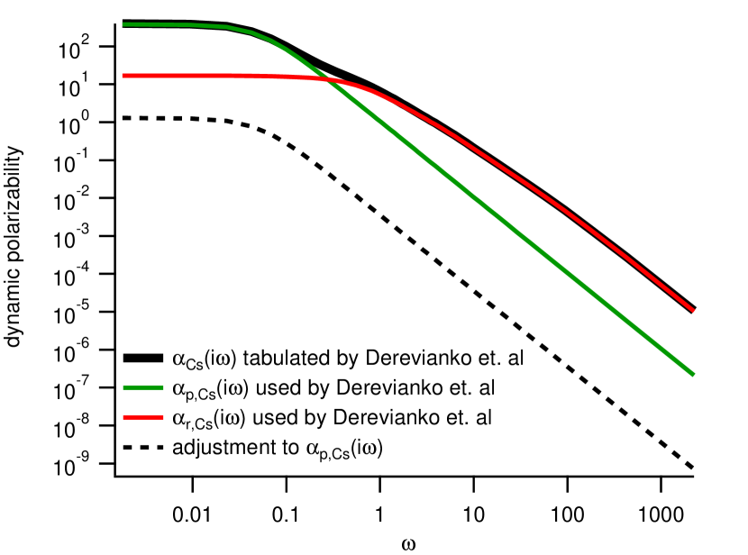
Figure 5: Cesium atom $\alpha_{tab}(i\omega)$ tabulated in Derevianko et al. (2010) (black line), and its decomposition into calculated $\alpha_{p}(i\omega)$ based on $\tau_{1/2}$ and $\tau_{3/2}$ values Volz and Schmoranzer (1996) with Eq. (2) (green line) and the residual $\alpha_{r}(i\omega)$ (red line). The black dotted line represents the adjustment to $\alpha_{p}(i\omega)$ when we substitute $\alpha(0)$ measurement into Eqn. (23).

Equation (23) shows how $C_{6}$ calculations depend on $\alpha_{r}(0)$ and $\alpha(i\omega)$ with opposite signs. This helps explain why uncertainty in $\alpha_{r}$ propagates to uncertainty in $C_{6}$ with a somewhat reduced impact. For example, if $\alpha_{r}$ accounts for 15% of $C_{6}$, and $\alpha_{r}$ itself has an uncertainty of 5%, one might naievely expect that uncertainty in $C_{6}$ due to uncertainty in $\alpha_{r}$ would be 0.75%. However, using Eqn. (23) one can show that the uncertainty in $C_{6}$ is smaller (only 0.48% due to $\alpha_{r}$). To explain this, if a theoretical $\alpha_{r}$ is incorrect, say a bit too high, then when we subtract this from the measured $\alpha(0)$ we will deduce an $\alpha_{p}(0)$ that is too small, and the error from this contribution to $C_{6}$ has the opposite sign from the error caused by adding back $\alpha_{r}(i\omega)$ in (23).

We can also rewrite Eqn. (23) by adding and subtracting the tabulated $\alpha_{p}(i\omega)$ so that $C_{6}$ depends explicitly only on the measured and tabulated (total) polarizabilities.

$$C_{6}=\frac{3\hbar}{\pi}\int_{0}^{\infty}\left[[\alpha(0)-\alpha_{tab}(0)]\frac{\alpha_{p}(i\omega)}{\alpha_{p}(0)}+\alpha_{tab}(i\omega)\right]^{2}d\omega$$ (25)

where $\alpha_{tab}(i\omega)$ and $\alpha_{tab}(0)$ refer to values tabulated by Derevianko et al.This way $C_{6}$ does not explicitly depend on $\alpha_{r}$.

Using Eqn. (25), or equivalently Eqns. (23) and (24), our calculated $C_{6}$ values for Rb and Cs agree with recent theoretical and experimental $C_{6}$ values, as shown in Fig. 6. For K, our predicted $C_{6}$ is different from that measured by D’Errico et al.using Feshbach resonances by roughly 3$\sigma$. Of course, this discrepancy may be at least partly explained by statistical errors in the $C_{6}$ and $\alpha(0)$ measurements for K atoms. In the next section, however, we will explore how error in $\alpha_{r}(i\omega)$ used to construct $\alpha_{tab}(i\omega)$ for K could partly explain this discrepancy.

Table 4: Homonuclear van der Waals $C_{6}$ coefficients, in atomic units, calculated using experimental static polarizabilities shown in Table 1 and tabulated dynamic polarizabilities from Derevianko et al. (2010). The two contributions to the uncertainty $\delta_{\alpha(0)}$ and $\delta_{\alpha_{r}(0)}$ for each $C_{6}$ value are, respectively, due to the uncertainties in measured $\alpha(0)$ and uncertainties estimated for Derevianko et al.’s values for $\alpha_{r}(i\omega)$ used to calculate $\alpha_{tab}(i\omega)$. Derevianko et al.Derevianko et al. (1999) reported uncertainty in $\alpha_{r}(0)$ by using "an estimated 5% error for the core polarizabilities, and a 10% error for the remaining contributions to $\alpha_{r}(0)$." Several other authors also estimate 5% or 2% error for $\alpha_{\mathrm{core}}$.

Atom	$C_{6}$	$\delta_{\alpha(0)}$	$\delta_{\alpha_{r}(0)}$
Na	1558(11)	10	1
K	3884(16)	7	14
Rb	4724(31)	10	130
Cs	6879(15)	13	7

To interpret the $C_{6}$ values that we report in Table 4, we compare these semi-empirical results to direct measurements and earlier predictions of $C_{6}$ in Fig. 6. One sees that the uncertainty of $C_{6}$ measurements that we report based on atom interferometry measurements of polarizability are comparable to direct measurements D’Errico et al. (2007); van Kempen et al. (2002); Chin et al. (2004) and slightly more precise than previous semi-empirical predictions Derevianko et al. (2010) .

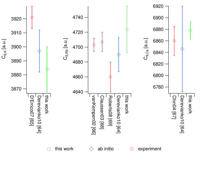
Figure 6: Theoretical Derevianko et al. (2010) and experimental D’Errico et al. (2007); van Kempen et al. (2002); Claussen et al. (2003); Roberts et al. (1998); Chin et al. (2004) $C_{6}$ values of K, Rb, and Cs from several different sources and the $C_{6}$ values determined in this article from polarizability measurements Gregoire et al. (2015). The experimental $C_{6}$ values were all determined from Feshbach resonance data.

4 Determining residual polarizabilities empirically

4.1 Using combinations of $\alpha(0)$ and $\tau$ measurements to report $\alpha_{r}$ values

While in Section 3 we demonstrated how to report atomic lifetimes from polarizability measurements and theoretical values for $\alpha_{r}(0)$, here we invert this procedure and use combinations of $\alpha(0)$, $\tau_{1/2}$, and $\tau_{3/2}$ measurements to place constraints on $\alpha_{r}(0)$. For this, we solve Eqn. (8) for $\alpha_{r}(0)$:

$$\alpha_{r}(0)=\alpha(0)-2\pi\epsilon_{0}c^{3}\left[\frac{\tau_{1/2}^{-1}}{\omega_{D1}^{4}}+2\frac{\tau_{3/2}^{-1}}{\omega_{D2}^{4}}\right]$$ (26)

Fig. 7 shows the difference between polarizability measurements $\alpha(0)$ and the inferred contribution to polarizability from the principal transitions $\alpha_{p}(0)$ based on lifetime measurements. We take the weighted average of $\alpha_{p}(0)$ based on a collection of available lifetime measurements, and we use the weighted average of the two high-precision $\alpha_{\textrm{Cs}}(0)$ measurements. We obtain $\alpha_{r,\textrm{Li}}(0)$ = 2(1), $\alpha_{r,\textrm{Na}}(0)$ = 2.0(5), $\alpha_{r,\textrm{K}}(0)$ = 5.4(4), $\alpha_{r,\textrm{Rb}}(0)$ = 11.4(5), and $\alpha_{r,\textrm{Cs}}(0)$ = 18.1(5). This analysis shows significantly nonzero $\alpha_{r}(0)$ values for Li, Na, K, Rb, and Cs based entirely on experimental data.

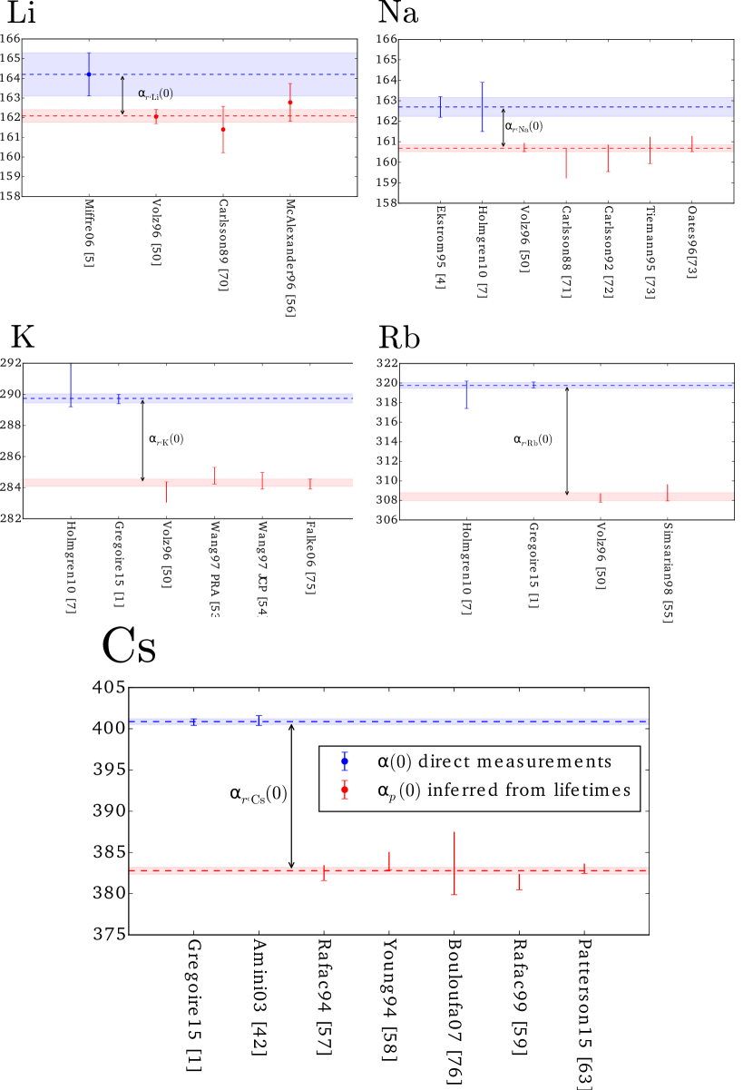
Figure 7: Differences between recent $\alpha(0)$ measurements Miffre et al. (2006); Ekstrom et al. (1995); Holmgren et al. (2010); Gregoire et al. (2015); Amini and Gould (2003) and an average of $\alpha_{p,\mathrm{Cs}}$ values calculated from lifetime measurements Volz and Schmoranzer (1996); Carlsson and Sturesson (1989); McAlexander et al. (1996); Carlsson (1988); Carlsson et al. (1992); Tiemann et al. (1996); Oates et al. (1996); Wang et al. (1997a, b); Falke et al. (2006); Simsarian et al. (1998); Rafac et al. (1994); Young et al. (1994); Bouloufa et al. (2007); Rafac et al. (1999); Patterson et al. (2015) and $R$ values Johnson et al. (2008); Volz and Schmoranzer (1996); Trubko (2016); Leonard et al. (2015); Rafac and Tanner (1998). The uncertainties on those averages are used to calculate the resulting uncertainties in $\alpha_{r}(0)$.

For Cs, this approach is sufficiently precise to empirically measure $\alpha_{r}(0)$ with 3% uncertainty, which is similar to the uncertainty of theoretical values Safronova et al. (2006); Derevianko and Porsev (2002). The width of the blue and red bands in Fig. 7 indicate the contributions to this uncertainty from the atom interferometry polarizability measurements and the uncertainty contributions from lifetime measurements. In order to improve the accuracy of $\alpha(0)$ reported this way one would require improvements in both the polarizability measurements and the lifetime measurements.

We can use a similar approach by combining polarizability measurements with ab initio $|D_{ik}|$ calculations. One of the highest-accuracy calculations of $|D_{D1}|$ was reported for Cs by Porsev et al.Porsev et al. (2010) in order to help interpret atomic parity violation experiments. This $|D_{D1}|$ can be combined with $R$ Rafac and Tanner (1998) using equations (9) and (17) as

$$\alpha_{r}(0)=\alpha(0)-\frac{|D_{D1}|^{2}}{3\hbar}\left[\frac{1}{\omega_{D1}}+\frac{R}{\omega_{D2}}\right]$$ (27)

This approach produces a somewhat lower value of $\alpha_{r}(0)$ = 16.5(4) with about 2.5% uncertainty. We compare the results using lifetimes and this result using the ratio of line strengths ($R$) and a calculated dipole matrix element with other results in Fig. 9 at the end of this section.

4.2 Using combinations of $\alpha(0)$ and $C_{6}$ measurements to report $\alpha_{r}$ values

Earlier in Section 3.2 we demonstrated how to calculate van der Waals $C_{6}$ coefficients from polarizability measurements and assumptions about residual polarizabilities. We can also invert this procedure, and analyze combinations of $\alpha(0)$ and $C_{6}$ measurements in order to place constraints on $\alpha_{r}(0)$. For this we will assume the spectral function $\alpha_{r}(i\omega)/\alpha_{r}(0)$ is sufficiently known and simply factor out an overall scale factor for the static residual polarizability from the formula for $C_{6}$ Eqn. (23) as follows:

$$C_{6}=\frac{3\hbar}{\pi}\int_{0}^{\infty}\left[(\alpha(0)-\alpha_{r}(0))\frac{\alpha_{p}(i\omega)}{\alpha_{p}(0)}+\alpha_{r}(0)\frac{\tilde{\alpha}_{r}(i\omega)}{\tilde{\alpha}_{r}(0)}\right]^{2}d\omega$$ (28)

where $\tilde{\alpha}_{r}(i\omega)$ and $\tilde{\alpha}_{r}(0)$ refer to values we infer from Eqn. (24) using values tabulated by Derevianko et al.We then plot predictions for $C_{6}$ versus predictions for $\alpha(0)$ parametric in hypothetical $\alpha_{p}(0)$ for different values of $\alpha_{r}(0)$. This is shown in Fig. 8 along with measurements of $C_{6}$ (red) and $\alpha(0)$ (blue). Even on the graph with a large domain (small plots in Fig. 8) where one sees the generally quadratic dependence of $C_{6}$ on $\alpha(0)$, it is evident that a model with $\alpha_{r}(0)$=0 is incompatible with the data. On the expanded region of interest (larger plots in Fig. 8), one sees the intersection of $C_{6}$ and $\alpha(0)$ measurements specifies a value of $\alpha_{r}(0)$. For Cs, we obtain an $\alpha_{r}(0)$ = 16.8(8) that is consistent with $\alpha_{r}(0)$ found from the other two methods we have presented so far in Section 4. This method is valuable because it relies on independent measurements of $C_{6}$ and $\alpha(0)$ to provide an empirical measurement of the size of $\alpha_{r}$.

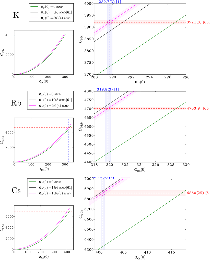
Figure 8: $C_{6}$ versus $\alpha(0)$ for small deviations about experimental values of $\alpha(0)$ Gregoire et al. (2015). The different curves correspond to different values of $\alpha_{r}(0)$: The pink curve corresponds to the value of $\alpha_{r}(0)$ inferred from experimental measurements of $C_{6}$ and $\alpha(0)$ Gregoire et al. (2015), and the error bands on that curve represent the resulting uncertainty in $\alpha_{r}(0)$ due to uncertainty in $C_{6}$ and $\alpha(0)$. The black curve corresponds to the values of $\alpha(i\omega)$ tabulated by Derevianko et al.Derevianko et al. (2010). Finally, the green line corresponds to $\alpha_{r}(0)=0$, and the inset on each plot shows $C_{6}$ versus $\alpha(0)$ for a wider range of $\alpha(0)$. For these plots, we used the $C_{6,\textrm{K}}$ measurement by D’Errico et al.D’Errico et al. (2007), $C_{6,\textrm{Rb}}$ by van Kempen et al.van Kempen et al. (2002), and $C_{6,\textrm{Cs}}$ by Chin et al.Chin et al. (2004). In the smaller plots, we can see that $C_{6}$ versus $\alpha(0)$ is approximately quadratic.

These plots show the values of $\alpha_{r}(0)$ and the corresponding uncertainties that we would infer using experimental values (and their uncertainties) of $\alpha(0)$ and $C_{6}$. From these studies we find a best fit $\alpha_{r}(0)$ of 8.0(4) for K, 9.6(4) for Rb, and 16.8(8) for Cs. The analysis for K highlights how the discrepancy between D’Errico et al.’s D’Errico et al. (2007) $C_{6,\textrm{K}}$ measurement and the $C_{6,\textrm{K}}$ that we infer from our $\alpha(0)$ measurement Gregoire et al. (2015) could be explained in part by error in assumed $\alpha_{\textrm{K}}(0)$.

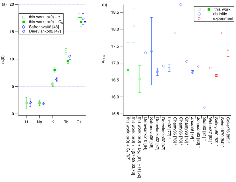
Figure 9: (a): $\alpha_{r}(0)$ values deduced by combining $\alpha(0)$ measurements Miffre et al. (2006); Ekstrom et al. (1995); Holmgren et al. (2010); Gregoire et al. (2015); Amini and Gould (2003) with either $C_{6}$ measurements D’Errico et al. (2007); van Kempen et al. (2002); Chin et al. (2004) or principal transition lifetime measurements Volz and Schmoranzer (1996); Carlsson and Sturesson (1989); McAlexander et al. (1996); Carlsson (1988); Carlsson et al. (1992); Tiemann et al. (1996); Oates et al. (1996); Wang et al. (1997a, b); Falke et al. (2006); Simsarian et al. (1998); Rafac et al. (1994); Young et al. (1994); Bouloufa et al. (2007); Rafac et al. (1999); Patterson et al. (2015) and $R$ values Johnson et al. (2008); Volz and Schmoranzer (1996); Trubko (2016); Leonard et al. (2015); Rafac and Tanner (1998). These inferred values are compared to the theoretical $\alpha_{r}(0)$ values we used elsewhere in this work by Safronova et al.Safronova et al. (2006) and Derevianko and Porsev Derevianko and Porsev (2002). (b): $\alpha_{r,\textrm{Cs}}(0)$ values deduced by combining measured $\alpha_{\textrm{Cs}}(0)$ Gregoire et al. (2015) with either measured $C_{6,\textrm{Cs}}$ Chin et al. (2004), principal transition lifetime Rafac et al. (1994); Young et al. (1994); Bouloufa et al. (2007); Rafac et al. (1999); Patterson et al. (2015) and $R_{\mathrm{Cs}}$ Rafac and Tanner (1998) measurements, or $\alpha_{p,\mathrm{Cs}}(0)$ inferred from calculated $|D_{\mathrm{D1,Cs}}|$ Porsev et al. (2010) and measured $R_{\mathrm{Cs}}$ Rafac and Tanner (1998). These inferred values are compared to several theoretical calculations Derevianko et al. (2010); Safronova et al. (2006); Derevianko and Porsev (2002); Lim et al. (2002); Ghanty and Ghosh (1996); Zhou and Norcross (1989); Johnson et al. (1983); Stott and Zaremba (1980) and Cs ion polarizability measurements Weber and Sansonetti (1987); Safinya et al. (1980); Schmidt et al. (1979); Coker (1976). The asterisk (*) indicates that the indicated references provided $\alpha_{\mathrm{core}}$ values which we converted to $\alpha_{r}(0)$ values by adding $\alpha_{v^{\prime}}+\alpha_{cv}=1.81-0.72=1.09$ (in atomic units).

Table 5: $\alpha_{r}(0)$ values deduced by combining $\alpha(0)$ measurements Miffre et al. (2006); Ekstrom et al. (1995); Holmgren et al. (2010); Gregoire et al. (2015); Amini and Gould (2003) with either $C_{6}$ measurements D’Errico et al. (2007); van Kempen et al. (2002); Chin et al. (2004), principal transition lifetime measurements Volz and Schmoranzer (1996); Carlsson and Sturesson (1989); McAlexander et al. (1996); Carlsson (1988); Carlsson et al. (1992); Tiemann et al. (1996); Oates et al. (1996); Wang et al. (1997a, b); Falke et al. (2006); Simsarian et al. (1998); Rafac et al. (1994); Young et al. (1994); Bouloufa et al. (2007); Rafac et al. (1999); Patterson et al. (2015) and $R$ values Johnson et al. (2008); Volz and Schmoranzer (1996); Trubko (2016); Leonard et al. (2015); Rafac and Tanner (1998), or $|D_{D1}|$ Porsev et al. (2010) and $R$ values Rafac and Tanner (1998). These inferred values are compared to the theoretical $\alpha_{r}(0)$ values we used elsewhere in this work by Safronova et al.Safronova et al. (2006) and Derevianko and Porsev Derevianko and Porsev (2002).

atom	$\alpha(0)+\tau$ [$+R$]	$\alpha(0)+C_{6}$	$\alpha(0)+|D_{D1}|+R$	ab initio
Li	2(1)			2.04(69) Safronova et al. (2006)
Na	2.0(5)			1.86(12) Safronova et al. (2006)
K	5.4(4)	8.0(4)		6.23(33) Safronova et al. (2006)
Rb	11.4(5)	9.6(4)		10.54(60) Safronova et al. (2006)
Cs	18.1(5)	16.8(8)	16.5(4)	17.35(100) Safronova et al. (2006)	16.74(11) Derevianko and Porsev (2002)

Fig. 9a shows the $\alpha_{r,\textrm{Cs}}(0)$ values we inferred from lifetime measurements, van der Waals $C_{6}$ coefficients, and Porsev et al.’s calculated $|D_{D1,\mathrm{Cs}}|$. Our results are compared to ab initio calculations of $\alpha_{r,\textrm{Cs}}(0)$ Derevianko et al. (2010); Safronova et al. (2006); Derevianko and Porsev (2002) as well as ab initio calculations of $\alpha_{\mathrm{core,Cs}}$ Lim et al. (2002); Ghanty and Ghosh (1996); Zhou and Norcross (1989); Johnson et al. (1983); Stott and Zaremba (1980) to which we added $\alpha_{v^{\prime}}+\alpha_{cv}$. Also among the comparisons in Fig. 9a are measurements of Cs⁺ ionic polarizability Weber and Sansonetti (1987); Safinya et al. (1980); Schmidt et al. (1979); Coker (1976), which approximates $\alpha_{\mathrm{core,Cs}}$, again adjusted by adding $\alpha_{v^{\prime}}+\alpha_{cv}$. Fig. 9b shows our results alongside the ab initio $\alpha_{r}(0)$ values calculated by Safronova et al.Safronova et al. (2006) and Derevianko and Porsev Derevianko and Porsev (2002) for Li, Na, K, Rb, and Cs.

Fig. 9 shows some disagreement between our $\alpha(0)+\tau$ and $\alpha(0)+C_{6}$ methods, especially with regard to K and Rb. There are several possible contributors to such disagreement. While the $\alpha(0)+\tau$ results were based on an average of several, independently-measured lifetimes, both of our methods relied on only one (or, in the case of Cs, two) $\alpha(0)$ measurements and our $\alpha(0)+C_{6}$ method relied on a single $C_{6}$ measurement. Therefore, statistical variation or systematic errors that were not accounted for in those $\alpha(0)$ or $C_{6}$ measurements could have a significant effect on our reported $\alpha_{r}(0)$. Also, it is important to note that our $\alpha(0)+C_{6}$ method relied on a single set of $\alpha(i\omega)$ calculated using one specific theoretical approach Derevianko et al. (2010), and that there are other theoretical approaches that could lead to different values of $\alpha(i\omega)$.

The uncertainties in ab initio $\alpha_{r}(0)$ predictions by Safronova et al.Safronova et al. (2006) and Derevianko and Porsev Derevianko and Porsev (2002) are comparable to or smaller than the uncertainties on our fully-empirical ($\alpha(0)+\tau$) and semi-empirical ($\alpha(0)+C_{6}$) results. This fact, combined with the aforementioned possible contributors to disagreement between our results, suggests that ab initio methods are still the prefered way of obtaining $\alpha_{r}(0)$ values for use in other analyses. Even so, it is valuable to develop the methods of analysis demonstrated in this paper so that when more accurate $\alpha(0)$, $\tau$, and $C_{6}$ measurements become available, then $\alpha_{r}(0)$ can be determined with higher accuracy using these methods.

The theoretical $\alpha_{r}(0)$ predictions by Safronova et al. Safronova et al. (2006) have an uncertainty of 6%, which is just slightly larger than the 5% or 3% uncertainties of the experimental $\alpha_{r}(0)$ determinations that we reported for Cs in Sections 4.1 and 4.2. However, we acknowledge that there is a 10% deviation between the all-experimental result for $\alpha_{r,\textrm{Cs}}(0)$ reported in Section 4.1 using $\alpha(0)$ and $\tau$ measurements as compared to the semi-empirical result for $\alpha_{r,\textrm{Cs}}(0)$ that we reported in Section 4.2 using $\alpha(0)$ and $C_{6}$ measurements combined with the theoretical spectral function $\alpha_{r}(i\omega)/\alpha_{r}(0)$. Furthermore, the uncertainty in the theoretical $\alpha_{r,\textrm{Cs}}(0)$ prediction by Derevianko and Porsev Derevianko and Porsev (2002) is significantly smaller, approximately 0.6% (and this was partly verified with independent measurements of $\alpha_{\mathrm{core}}$ using Rydberg spectroscopy Zhou and Norcross (1989)). So, it is possible that ab initio methods are still the preferred way of obtaining $\alpha_{r}(0)$ values for use in other analyses. Even so, we conclude that it is valuable to develop the methods of analysis demonstrated in this paper so that when more accurate $\alpha(0)$, $\tau$, and $C_{6}$ measurements become available, then $\alpha_{r}(0)$ can be determined with higher accuracy using these methods. In the future, combining measurements of $\alpha_{\mathrm{core}}$ from Rydberg spectroscopy with higher accuracy measurements of $\alpha_{r}(0)$ could provide more direct constraints on $\alpha_{v^{\prime}}+\alpha_{cv}$, and thus $\alpha_{\mathrm{tail}}$.

5 Discussion

In this paper we reported measurements of the static polarizabilities of K, Rb, and Cs atoms with reduced uncertainties. We made these measurements with an atom interferometer and an electric field gradient using data originally reported in [1]. We described in Section 2 how we reduced the systematic uncertainty in $\alpha(0)$ measurements from 0.15% to 0.10% by improving the calibration of the electric field. To our knowledge, these are now the most precise measurements of atomic polarizabilities that have been made using any method for K, Rb, and Cs atoms. For Cs in particular, the improvement described in this paper enabled us to report a value of $\alpha_{\textrm{Cs}}(0)$ with slightly smaller uncertainty than Amini and Gould’s measurement of $\alpha_{\textrm{Cs}}(0)$ that they obtained using an atomic fountain experiment Amini and Gould (2003). Currently, this means that atom interferometer experiments have made the most accurate measurements of atomic polarizabilities for all of the alkali metal atoms Li, Na, K, Rb, and Cs.

In Section 3 we demonstrated how to analyze these measurements of atomic polarizabilities in order to infer oscillator strengths, lifetimes, transition matrix elements, line strengths, and van der Waals $C_{6}$ coefficients for all the alkali metal atoms, as we did in Tables 2 and 4. We referred to the idea chart in Fig. 1 to review how these quantities are interrelated, and we described this more explicitly with Eqns. 1-17 and 19-25. Building on these interrelationships, we specifically used measurements of static polarizabilities obtained with atom interferometry, empirical ratios of line strengths $R$ (some of which were also obtained with atom interferometry), and theoretical values for residual polarizabilities in order to deduce the lifetimes of excited $np_{J}$ states for all of the alkali metal atoms with unprecedented accuracy. These methods also allow us to use static polarizability measurements as a semi-empirical benchmark to test ab initio predictions of principal $ns$-$np_{J}$ transition matrix elements for alkali metal atoms. Furthermore, we used these methods to test the extent to which measurements of different atomic properties such as lifetimes, branching ratios, line strengths, polarizabilities, and van der Waals interactions agree with one another, as shown in Figs. 4 and 6.

Then in Section 4 we explored new methods to infer residual polarizability $\alpha_{r}(0)$ values by combining measurements of atomic polarizabilities with independent measurements of lifetimes or $C_{6}$ coefficients. This constitutes a novel, all-experimental method to test several theoretical $\alpha_{r}(0)$ predictions. Using this approach it is clear that atom interferometry measurements of atomic polarizabilities are sufficiently precise to detect non-zero residual polarizabilities for all of the alkali metal atoms, and can measure $\alpha_{r}(0)$ with as little as 3% uncertainty for Cs atoms. This procedure also provides a motivation for next generation $C_{6}$, $\alpha(0)$, $\tau$, and tune-out wavelength measurements that can be combined with one another to more accurately determine $\alpha_{r}(0)$ values that are needed in order to test atomic structure calculations that are relevant for interpreting atomic parity violation and atomic clocks.

6 Acknowledgements

This work is supported by NSF Grant No. 1306308 and a NIST PMG. M.D.G. and R.T. are grateful for NSF GRFP Grant No. DGE-1143953 for support. N.B. acknowledges support from the NASA Space Grant Consortium at the University of Arizona.

Appendix A

Table 6: Contributions to residual polarizability $\alpha_{r}(0)=\alpha_{v^{\prime}}(0)+\alpha_{\mathrm{core}}(0)+\alpha_{cv}(0)$ in atomic units. The quantity $\alpha_{v^{\prime}}(0)$ is the sum of all the contributions from the valence electron $ns$-$n^{\prime}p_{J}$ transitions with $n^{\prime}>n$ using Eqn. (1). This includes $\alpha_{\mathrm{tail}}(0)$. Values in bold are used to produce the results presented in Table 2 are in bold.

atom	$\alpha_{v^{\prime}}(0)$	$\alpha_{\mathrm{core}}(0)$		$\alpha_{cv}(0)$	$\alpha_{r}(0)$
Li		0.189(9)	Johnson et al. (1983) (b)		$\mathbf{2.04(69)}$	Safronova et al. (2006)
Li		0.192	Johnson and Cheng (1996)
Na	0.81 (a)	0.94(5)	Johnson et al. (1983) (b)
Na		1.00(4)	Lim et al. (2002)		$\mathbf{1.86(12)}$	Safronova et al. (2006)
K	0.72 (a)	5.46(27)	Johnson et al. (1983) (b)
K	0.90 Safronova and Safronova (2008)	5.50	Safronova and Safronova (2008)
K		5.52(4)	Lim et al. (2002)
K		5.50	Safronova et al. (2013)	-0.18 Safronova et al. (2013)	$\mathbf{6.26(33)}$	Safronova et al. (2006)
Rb	1.32 (a)	9.08(45)	Johnson et al. (1983) (b)
Rb		9.11(4)	Lim et al. (2002)		10.70(22)	Leonard et al. (2015) (c)
Rb		9.11(4)	Safronova et al. (2004)	-0.30 Safronova et al. (2004)	$\mathbf{10.54(60)}$	Safronova et al. (2006)
Cs	1.60 (a)	15.8(8)	Johnson et al. (1983) (b)	-0.72 Derevianko and Porsev (2002)	17.35(100)	Safronova et al. (2006)
Cs		15.8(1)	Lim et al. (2002)		16.91	Derevianko and Porsev (2002)
Cs	1.81 Derevianko and Porsev (2002)	15.81	Derevianko and Porsev (2002)		$\mathbf{16.74(11)}$	Derevianko and Porsev (2002)
Cs		16.3(2)	Coker (1976) (d)
Cs		15.17	Rosseinsky (1994) (d)
Cs		15.54(3)	Safinya et al. (1980) (e)
Cs		15.82(3)	Ruff et al. (1980) (e)
Cs		15.770(3)	Weber and Sansonetti (1987) (e)
Cs		17.64	Ghanty and Ghosh (1996) (f)

^(a) Calculated using $f_{ik}$ values from NIST NIST for $n-n^{\prime}$ transitions with $n^{\prime}=n+1$ to $n+5$.
^(b) For $\alpha_{\mathrm{core}}$ from Johnson et al. (1983) we list a fractional uncertainty of 5% as suggested in reference Safronova et al. (2004).
^(c) Reference Leonard et al. (2015) calculated ($\alpha_{\mathrm{core}}+\alpha_{cv}$) = 8.71(9) and $\alpha_{r}=10.70(22)$ at $\omega=2\pi c/790$nm.
^(d) from studies of ions in solid crystals
^(e) from Rydberg spectroscopy data
^(f) A result from DFT calculations

References

- Berman (1997) Berman, P., Ed. Atom Interferometry; Academic Press: San Diego, 1997.
- Cronin et al. (2009) Cronin, A.D.; Schmiedmayer, J.; Pritchard, D.E. Optics and interferometry with atoms and molecules. Rev. Mod. Phys. 2009, 81, 1051.
- Gregoire et al. (2015) Gregoire, M.D.; Hromada, I.; Holmgren, W.F.; Trubko, R.; Cronin, A.D. Measurements of the ground-state polarizabilities of Cs, Rb, and K using atom interferometry. Phys. Rev. A 2015, 92, 052513.
- Ekstrom et al. (1995) Ekstrom, C.R.; Schmiedmayer, J.; Chapman, M.S.; Hammond, T.D.; Pritchard, D.E. Measurement of the electric polarizability of sodium with an atom interferometer. Phys. Rev. A 1995, 51, 3883.
- Miffre et al. (2006) Miffre, A.; Jacquey, M.; Büchner, M.; Trénec, G.; Vigué, J. Atom interferometry measurement of the electric polarizability of lithium. Eur. Phys. J. D 2006, 38, 353.
- Berninger et al. (2007) Berninger, M.; Stefanov, A.; Deachapunya, S.; Arndt, M. Polarizability measurements of a molecule via a near-field matter-wave interferometer. Phys. Rev. A 2007, 76, 013607.
- Holmgren et al. (2010) Holmgren, W.F.; Revelle, M.C.; Lonij, V.P.A.; Cronin, A.D. Absolute and ratio measurements of the polarizability of Na, K, and Rb with an atom interferometer. Phys. Rev. A 2010, 81, 053607.
- Perreault and Cronin (2005) Perreault, J.D.; Cronin, A.D. Observation of atom wave phase shifts induced by van der Waals atom-surface interactions. Phys. Rev. Lett. 2005, 95, 133201.
- Lepoutre et al. (2009) Lepoutre, S.; Jelassi, H.; Lonij, V.P.A.; Trénec, G.; Büchner, M.; Cronin, a.D.; Vigué, J. Dispersive atom interferometry phase shifts due to atom-surface interactions. Europhys. Lett. 2009, 88, 20002.
- Lepoutre et al. (2011) Lepoutre, S.; Lonij, V.P.A.; Jelassi, H.; Trenec, G.; Buchner, M.; Cronin, A.D.; Vigue, J.; Trénec, G.; Büchner, M.; Vigué, J. Atom interferometry measurement of the atom-surface van der Waals interaction. Eur. Phys. J. D 2011, 62, 309.
- Holmgren et al. (2012) Holmgren, W.F.; Trubko, R.; Hromada, I.; Cronin, A.D. Measurement of a wavelength of light for which the energy shift for an atom vanishes. Phys. Rev. Lett. 2012, 109, 243004.
- Leonard et al. (2015) Leonard, R.H.; Fallon, A.J.; Sackett, C.A.; Safronova, M.S. High-precision measurements of the -line tune-out wavelength. Phys. Rev. A 2015, 92, 052501.
- Mitroy et al. (2010) Mitroy, J.; Safronova, M.S.; Clark, C.W. Theory and applications of atomic and ionic polarizabilities. J. Phys. B 2010, 44, 202001.
- Tang et al. (2009) Tang, L.Y.; Yan, Z.C.; Shi, T.Y.; Babb, J.F. Nonrelativistic ab initio calculations for 2 S 2, 2 P 2, and 3 D 2 lithium isotopes: Applications to polarizabilities and dispersion interactions. Physical Review A 2009, 79, 062712.
- Sahoo (2007) Sahoo, B. An ab initio relativistic coupled-cluster theory of dipole and quadrupole polarizabilities: Applications to a few alkali atoms and alkaline earth ions. Chemical Physics Letters 2007, 448, 144–149.
- Hamonou and Hibbert (2007) Hamonou, L.; Hibbert, A. Static and dynamic polarizabilities of Na-like ions. Journal of Physics B: Atomic, Molecular and Optical Physics 2007, 40, 3555.
- Deiglmayr et al. (2008) Deiglmayr, J.; Aymar, M.; Wester, R.; Weidemüller, M.; Dulieu, O. Calculations of static dipole polarizabilities of alkali dimers: Prospects for alignment of ultracold molecules. The Journal of chemical physics 2008, 129, 064309.
- Johnson et al. (2008) Johnson, W.; Safronova, U.; Derevianko, A.; Safronova, M. Relativistic many-body calculation of energies, lifetimes, hyperfine constants, and polarizabilities in Li 7. Physical Review A 2008, 77, 022510.
- Reinsch and Meyer (1976) Reinsch, E.A.; Meyer, W. Finite perturbation calculation for the static dipole polarizabilities of the atoms Na through Ca. Phys. Rev. A 1976, 14, 915.
- Tang (1976) Tang, K.T. Upper and lower bounds of two- and three-body dipole, quadrupole, and octupole van der Waals coefficients for hydrogen, noble gas, and alkali atom interactions. J. Chem. Phys. 1976, 64, 3063.
- Maeder and Kutzelnigg (1979) Maeder, F.; Kutzelnigg, W. Natural states of interacting systems and their use for the calculation of intermolecular forces (IV) Calculation of van der Waals coefficients between one-and two-valence-electron atoms in their ground states, as well as of polarizabilities, oscillator strength sums and related quantities, including correlation effects. Chemical Physics 1979, 42, 95–112.
- Christiansen and Pitzer (1982) Christiansen, P.A.; Pitzer, K.S. Reliable static electric dipole polarizabilities for heavy elements. Chem. Phys. Lett. 1982, 85, 434.
- Fuentealba (1982) Fuentealba, P. On the reliability of semiempirical pseudopotentials: dipole polarisability of the alkali atoms. Journal of Physics B: Atomic and Molecular Physics 1982, 15, L555.
- Müller et al. (1984) Müller, W.; Flesch, J.; Meyer, W. Treatment of intershell correlation effects in calculations by use of core polarization potentials. Method and application to alkali and alkaline earth atoms. J. Chem. Phys. 1984, 80, 3297.
- Kundu et al. (1986) Kundu, B.; Ray, D.; Mukherjee, P. Dynamic polarizabilities and Rydberg states of the sodium isoelectronic sequence. Physical Review A 1986, 34, 62.
- Kello et al. (1993) Kello, V.; Sadlej, A.J.; Faegri, K. Electron-correlation and relativistic contributions to atomic dipole polarizabilities: Alkali-metal atoms. Phys. Rev. A 1993, 47, 1715.
- Fuentealba and Reyes (1993) Fuentealba, P.; Reyes, O. Atomic softness and the electric dipole polarizability. J. Mol. Struct. THEOCHEM 1993, 282, 65.
- Marinescu et al. (1994) Marinescu, M.; Sadeghpour, H.; Dalgarno, A. Dispersion coefficients for alkali-metal dimers. Physical Review A 1994, 49, 982.
- Dolg (1996) Dolg, M. Fully relativistic pseudopotentials for alkaline atoms: Dirac–Hartree–Fock and configuration interaction calculations of alkaline monohydrides. Theor. Chim. Acta 1996, 93, 141.
- Patil and Tang (1997) Patil, S.H.; Tang, K.T. Multipolar polarizabilities and two- and three-body dispersion coefficients for alkali isoelectronic sequences. J. Chem. Phys. 1997, 106, 2298.
- Lim et al. (1999) Lim, I.S.; Pernpointner, M.; Seth, M.; Laerdahl, J.K.; Schwerdtfeger, P.; Neogrady, P.; Urban, M. Relativistic coupled-cluster static dipole polarizabilities of the alkali metals from Li to element 119. Phys. Rev. A 1999, 60, 2822.
- Safronova et al. (1999) Safronova, M.S.; Johnson, W.R.; Derevianko, A. Relativistic many-body calculations of energy levels, hyperfine constants, electric-dipole matrix elements and static polarizabilities for alkali-metal atoms. Phys. Rev. A 1999, 60, 27.
- Derevianko et al. (1999) Derevianko, A.; Johnson, W.R.; Safronova, M.S.; Babb, J.F. High-precision calculations of dispersion coefficients, static dipole polarizabilities, and atom-wall interaction constants for alkali-metal atoms. Phys. Rev. Lett. 1999, 82, 3589.
- Magnier and Aubert-Frécon (2002) Magnier, S.; Aubert-Frécon, M. Static dipolar polarizabilities for various electronic states of alkali atoms. J. Quant. Spectrosc. Radiat. Transf. 2002, 75, 121.
- Mitroy and Bromley (2003) Mitroy, J.; Bromley, M.W.J. Semiempirical calculation of van der Waals coefficients for alkali-metal and alkaline-earth-metal atoms. Phys. Rev. A 2003, 68, 052714.
- Safronova and Clark (2004) Safronova, M.S.; Clark, C.W. Inconsistencies between lifetime and polarizability measurements in Cs. Phys. Rev. A 2004, 69, 040501.
- Lim et al. (2005) Lim, I.S.; Schwerdtfeger, P.; Metz, B.; Stoll, H. All-electron and relativistic pseudopotential studies for the group 1 element polarizabilities from K to element 119. J. Chem. Phys. 2005, 122, 104103.
- Arora et al. (2007) Arora, B.; Safronova, M.; Clark, C.W. Determination of electric-dipole matrix elements in K and Rb from Stark shift measurements. Physical Review A 2007, 76, 052516.
- Iskrenova-Tchoukova et al. (2007) Iskrenova-Tchoukova, E.; Safronova, M.S.; Safronova, U.I. High-precision study of Cs polarizabilities. J. Comput. Methods Sci. Eng. 2007, 7, 521.
- Safronova and Safronova (2008) Safronova, U.I.; Safronova, M.S. High-accuracy calculation of energies , lifetimes , hyperfine constants , multipole polarizabilities , and blackbody radiation shift in 39K. Phys. Rev. A 2008, 78, 052504.
- Safronova and Safronova (2011) Safronova, M.S.; Safronova, U.I. Critically evaluated theoretical energies, lifetimes, hyperfine constants, and multipole polarizabilities in 87Rb. Phys. Rev. A 2011, 83, 052508.
- Amini and Gould (2003) Amini, J.M.; Gould, H. High precision measurement of the static dipole polarizability of cesium. Phys. Rev. Lett. 2003, 91, 153001.
- Schwerdtfeger (2006) Schwerdtfeger, P. Atomic static dipole polarizabilities. In Atoms, Mol. Clust. Electr. Fields Theor. Approaches to Calc. Electr. Polariz.; 2006; pp. 1–32.
- (44) Schwerdtfeger, P. Table of experimental and calculated static dipole polarizabilities for the electronic ground states of the neutral elements (in atomic units). Cent. Theor. Chem. Phys. (CTCP), New Zeal. Inst. Adv. Study, Massey Univ. Auckl.
- Gould and Miller (2005) Gould, H.; Miller, T.M. Recent Developments in the Measurement of Static Electric Dipole Polarizabilities; Vol. 51, Elsevier Masson SAS, 2005; p. 343.
- Haynes (2014) Haynes, W.M. CRC Handbook of Chemistry and Physics; CRC Press, 2014.
- Derevianko and Porsev (2002) Derevianko, A.; Porsev, S.G. High-precision determination of transition amplitudes of principal transitions in Cs from van der Waals coefficient C6. Phys. Rev. A 2002, 65, 053403.
- Safronova et al. (2006) Safronova, M.S.; Arora, B.; Clark, C.W. Frequency-dependent polarizabilities of alkali-metal atoms from ultraviolet through infrared spectral regions. Phys. Rev. A 2006, 73, 022505.
- (49) NIST. NIST Atomic Spectra Database.
- Volz and Schmoranzer (1996) Volz, U.; Schmoranzer, H. Precision lifetime measurements on alkali atoms and on helium by beam–gas–laser spectroscopy. Phys. Scr. 1996, T65, 48.
- Trubko (2016) Trubko, R. Precision tune-out wavelength measurements with an atom interferometer. Prep. 2016.
- Rafac and Tanner (1998) Rafac, R.J.; Tanner, C.E. Measurement of the ratio of the cesium D-line transition strengths. Phys. Rev. A 1998, 58, 1087.
- Wang et al. (1997a) Wang, H.; Li, J.; Wang, X.T.; Williams, C.J.; Gould, P.L.; Stwalley, W.C. Precise determination of the dipole matrix element and radiative lifetime of the 39K 4p state by photoassociative spectroscopy. Phys. Rev. A 1997, 55, R1569.
- Wang et al. (1997b) Wang, H.; Gould, P.L.; Stwalley, W.C. Long-range interaction of the K(4s)+K(4p) asymptote by photoassociative spectroscopy. I. The pure long-range state and the long-range potential constants. J. Chem. Phys. 1997, 106, 7899.
- Simsarian et al. (1998) Simsarian, J.E.; Orozco, L.A.; Sprouse, G.D.; Zhao, W.Z. Lifetime measurements of the 7 levels of atomic francium. Phys. Rev. A 1998, 57, 2448.
- McAlexander et al. (1996) McAlexander, W.I.; Abraham, E.R.I.; Hulet, R.G. Radiative lifetime of the state of lithium. Phys. Rev. A 1996, 54, R5.
- Rafac et al. (1994) Rafac, R.J.; Tanner, C.E.; Livingston, A.E.; Kukla, K.W.; Berry, H.G.; Kurtz, C.A. Precision lifetime measurements of the 6 states in atomic cesium 1994. 50, 1976.
- Young et al. (1994) Young, L.; Hill, W.T.; Sibener, S.J.; Price, S.D.; Tanner, C.E.; Wieman, C.E.; Leone, S.R. Precision lifetime measurements of Cs 6 and 6 levels by single-photon counting. Phys. Rev. A 1994, 50, 2174.
- Rafac et al. (1999) Rafac, R.J.; Tanner, C.E.; Livingston, A.E.; Berry, H.G. Fast-beam laser lifetime measurements of the cesium 6p states. Phys. Rev. A 1999, 60, 3648.
- Derevianko and Porsev (2002) Derevianko, A.; Porsev, S.G. Determination of lifetimes of 6 P J levels and ground-state polarizability of Cs from the van der Waals coefficient C 6. Physical Review A 2002, 65, 053403.
- Porsev et al. (2010) Porsev, S.G.; Beloy, K.; Derevianko, A. Precision determination of weak charge of 133Cs from atomic parity violation. Phys. Rev. D 2010, 82, 036008.
- Porsev et al. (2009) Porsev, S.G.; Beloy, K.; Derevianko, A. Precision determination of electroweak coupling from atomic parity violation and implications for particle physics. Phys. Rev. Lett. 2009, 102, 181601.
- Patterson et al. (2015) Patterson, B.M.; Sell, J.F.; Ehrenreich, T.; Gearba, M.A.; Brooke, G.M.; Scoville, J.; Knize, R.J. Lifetime measurement of the cesium 6 P 3/2 level using ultrafast pump-probe laser pulses. Physical Review A 2015, 91, 012506.
- Derevianko et al. (2010) Derevianko, A.; Porsev, S.G.; Babb, J.F. Electric dipole polarizabilities at imaginary frequencies for hydrogen, the alkali-metal, alkaline-earth, and noble gas atoms. At. Data Nucl. Data Tables 2010, 96, 323.
- D’Errico et al. (2007) D’Errico, C.; Zaccanti, M.; Fattori, M.; Roati, G.; Inguscio, M.; Modugno, G.; Simoni, A. Feshbach resonances in ultracold K(39). New J. Phys. 2007, 9, 223.
- van Kempen et al. (2002) van Kempen, E.G.M.; Kokkelmans, S.J.J.M.F.; Heinzen, D.J.; Verhaar, B.J. Interisotope determination of ultracold rubidium interactions from three high-precision experiments. Phys. Rev. Lett. 2002, 88, 093201.
- Chin et al. (2004) Chin, C.; Vuletić, V.; Kerman, A.J.; Chu, S.; Tiesinga, E.; Leo, P.J.; Williams, C.J. Precision feshbach spectroscopy of ultracold Cs2. Phys. Rev. A 2004, 70, 032701.
- Claussen et al. (2003) Claussen, N.R.; Kokkelmans, S.J.J.M.F.; Thompson, S.T.; Donley, E.A.; Hodby, E.; Wieman, C.E. Very-high-precision bound-state spectroscopy near a 85Rb Feshbach resonance. Phys. Rev. A 2003, 67, 060701.
- Roberts et al. (1998) Roberts, J.L.; Claussen, N.R.; Burke, J.P.; Greene, C.H.; Cornell, E.A.; Wieman, C.E. Resonant Magnetic Field Control of Elastic Scattering in Cold 85Rb. Phys. Rev. Lett. 1998, 81, 5109.
- Carlsson and Sturesson (1989) Carlsson, J.; Sturesson, L. Accurate time-resolved laser spectroscopy on lithium atoms. Zeitschrift für Physik D Atoms, Molecules and Clusters 1989, 14, 281–287.
- Carlsson (1988) Carlsson, J. Accurate time-resolved laser spectroscopy on sodium and bismuth atoms. Zeitschrift für Physik D Atoms, Molecules and Clusters 1988, 9, 147–151.
- Carlsson et al. (1992) Carlsson, J.; Jönsson, P.; Sturesson, L.; Fischer, C.F. Multi-configuration Hartree-Fock calculations and time-resolved laser spectroscopy studies of hyperfine structure constants in sodium. Physica Scripta 1992, 46, 394.
- Tiemann et al. (1996) Tiemann, E.; Knöckel, H.; Richling, H. Long-range interaction at the asymptote 3s+3 of Na2. Zeitschrift für Physik D Atoms, Molecules and Clusters 1996, 37, 323–332.
- Oates et al. (1996) Oates, C.W.; Vogel, K.R.; Hall, J.L. High Precision Linewidth Measurement of Laser-Cooled Atoms: Resolution of the Na Lifetime Discrepancy. Phys. Rev. Lett. 1996, 76, 2866–2869.
- Falke et al. (2006) Falke, S.; Sherstov, I.; Tiemann, E.; Lisdat, C. The state of up to the dissociation limit. J. Chem. Phys. 2006, 125, 224303.
- Bouloufa et al. (2007) Bouloufa, N.; Crubellier, A.; Dulieu, O. Reexamination of the pure long-range state of Cs2: Prediction of missing levels in the photoassociation spectrum. Phys. Rev. A 2007, 75, 052501.
- Lim et al. (2002) Lim, I.S.; Laerdahl, J.K.; Schwerdtfeger, P. Fully relativistic coupled-cluster static dipole polarizabilities of the positively charged alkali ions from Li+ to 119+. J. Chem. Phys. 2002, 116, 172.
- Ghanty and Ghosh (1996) Ghanty, T.K.; Ghosh, S.K. A new simple approach to the polarizability of atoms and ions using frontier orbitals from the Kohn-Sham density functional theory. Journal of Molecular Structure: THEOCHEM 1996, 366, 139–144.
- Zhou and Norcross (1989) Zhou, H.L.; Norcross, D.W. Improved calculation of the quadratic Stark effect in the 6 state of Cs. Phys. Rev. A 1989, 40, 5048–5051.
- Johnson et al. (1983) Johnson, W.; Kolb, D.; Huang, K.N. Electric-dipole, quadrupole, and magnetic-dipole susceptibilities and shielding factors for closed-shell ions of the He, Ne, Ar, Ni (Cu+), Kr, Pb, and Xe isoelectronic sequences. At. Data Nucl. Data Tables 1983, 28, 333.
- Stott and Zaremba (1980) Stott, M.J.; Zaremba, E. Linear-response theory within the density-functional formalism: Application to atomic polarizabilities. Phys. Rev. A 1980, 21, 12–23.
- Weber and Sansonetti (1987) Weber, K.H.; Sansonetti, C.J. Accurate energies of nS , nP , nD , nF , and nG levels of neutral cesium. Phys. Rev. A 1987, 35, 4650–4660.
- Safinya et al. (1980) Safinya, K.; Gallagher, T.; Sandner, W. Resonance measurements of f- h and f- i intervals in cesium using selective and delayed field ionization. Physical Review A 1980, 22, 2672.
- Schmidt et al. (1979) Schmidt, P.C.; Weiss, A.; Das, T.P. Effect of crystal fields and self-consistency on dipole and quadrupole polarizabilities of closed-shell ions. Phys. Rev. B 1979, 19, 5525–5534.
- Coker (1976) Coker, H. Empirical Free-Ion Polarizabilities of the Alkali Metal, Alkaline Earth Metal, and Halide Ions. J. Phys. Chem. 1976, 80, 2078.
- Johnson and Cheng (1996) Johnson, W.; Cheng, K. Relativistic configuration-interaction calculation of the polarizabilities of heliumlike ions. Physical Review A 1996, 53, 1375.
- Safronova et al. (2013) Safronova, M.S.; Safronova, U.I.; Clark, C.W. Magic wavelengths for optical cooling and trapping of potassium. Phys. Rev. A 2013, 87, 052504.
- Safronova et al. (2004) Safronova, M.S.; Williams, C.J.; Clark, C.W. Relativistic many-body calculations of electric-dipole matrix elements, lifetimes and polarizabilities in rubidium 2004. 69, 022509.
- Rosseinsky (1994) Rosseinsky, D.R. An electrostatics framework relating ionization potential (and electron affinity), electronegativity, polarizability, and ionic radius in monatomic species. Journal of the American Chemical Society 1994, 116, 1063–1066.
- Ruff et al. (1980) Ruff, G.; Safinya, K.; Gallagher, T. Measurements of the n= 15- 17 f- g intervals in Cs. Physical Review A 1980, 22, 183.