Beyond Zipf’s Law: The Lavalette Rank Function and Its Properties

Abstract

Although Zipf’s law is widespread in natural and social data, one often encounters situations where one or both ends of the ranked data deviate from the power-law function. Previously we proposed the Beta rank function to improve the fitting of data which does not follow a perfect Zipf’s law. Here we show that when the two parameters in the Beta rank function have the same value, the Lavalette rank function, the probability density function can be derived analytically. We also show both computationally and analytically that Lavalette distribution is approximately equal, though not identical, to the lognormal distribution. We illustrate the utility of Lavalette rank function in several datasets. We also address three analysis issues on the statistical testing of Lavalette fitting function, comparison between Zipf’s law and lognormal distribution through Lavalette function, and comparison between lognormal distribution and Lavalette distribution.

Introduction

It is said that a certain quantity follows a power law if the probability of observing it varies inversely as a power of this quantity. Power laws in data collected from natural or social phenomena are well documented Clauset et al. (2009). For instance, the asymptotic occurrence of power laws in critical phenomena and statistical physics has been widely studied Sornette (2006). In the same way, power law tails have been reported in the distribution of word frequency Zipf (1935), city sizes Gabaix (1999), fluctuations in financial market indexes Gopikrishnan et al. (1999), firm sizes in the U.S Axtell (2001), scientific citations Petersen et al. (2011); Petersen and Succi (2013) and there are many other examples. There are two common approaches in displaying a power law distribution: the histogram, which approximates the probability density function (pdf), and the rank-frequency plot, best known by the Zipf’s law for usage of words in human languages Zipf (1935); Li (2002).

Empirical data often exhibit good power-law distribution within a limited range, whereas one or both ends of the distribution may deviate from the ideal power law Stumpf and Porter (2012). It is a well known fact that any finite size system, that is well described by a power law, deviates from this behaviour due to finite size effects Laherre and Sornette (1998). In these systems, the power law ceases to hold in a certain region, where effects due to the finiteness of the system dominate the behaviour (for example, finite sample size or finite available energy). Therefore, it is natural to see deviations from power laws at the tails. However, the question remains of whether deviations are merely explained by finite size effects or if they call for a modification in the whole body of the distribution. This paper explores the second possibility. Modifying a power law by changing the functional form potentially may fit the systematic deviation. Previously, we proposed a rank-frequency function, inspired by the Beta density function Bowman and Shenton (2007), called Beta-like function Mansilla et al. (2007), or Discrete Generalized Beta Distribution (DGBD) Martínez-Mekler et al. (2009), or Cocho rank function Li and Miramontes (2011). The DGBD

$$x_{[r]}=C\frac{(N+1-r)^{b}}{r^{a}}$$ (1)

($x$: quantity of interest, $r$: rank, $N$: the maximum rank), contains the fitting parameters $a$ and $b$ and the normalization factor $C$. We previously proposed that the parameter $a$ is associated with the behaviour which leads to the power law, whereas $b$ is associated with the fluctuation in noise Martínez-Mekler et al. (2009). An example of the former is the inertial range in turbulence where energy is transferred between different length scales with the same rate, while an example of the latter is the dissipative range in turbulence Martínez-Mekler et al. (2009). Another example is in a conflicting dynamics called expansion-modification systems Li (1991), where $a>b$ when expansion dominates mutation and $b>a$ when mutation dominates Alvarez-Martinez et al. (2011). Eq.(1) modifies the power law rank function $1/r^{a}$ by a power of the reverse-rank $r_{2}=N+1-r$, and it converges to power law when $b=0$. DGBD often surpasses other two-parameter functions in fitting real data Li and Miramontes (2011); Li et al. (2010); Petersen et al. (2011), and achieved various degree of success in other applications Mansilla et al. (2007); del Río et al. (2008); Martínez-Mekler et al. (2009); Petersen et al. (2011); Li (2012a, b, 2013); Li et al. (2014); Ausloos (2014).

It is a well known fact that a quantity that follows a power law in the rank-frequency representation has a Pareto distribution Newman (2005). The widespread application of the DGBD raises the issue of whether it is the result from a well known pdf, such as the normal/Gaussian distribution. In this work, we show that for a special case of the DGBD, the Lavalette rank function where $a=b$ Lavalette (1996); Popescu (1997, 2003); Lavalette (2007); Voloshynovska (2011), the corresponding pdf can be derived analytically. The Lavalette rank function is also intrinsically connected, by an approximation, to the lognormal distribution. We offer both numerical evidence and an analytic proof.

The paper is organized in the following way: first we derive and characterize the pdf associated with the Lavalette rank function, which we call the Lavalette distribution, and show that it is approximately equal to the lognormal distribution over a relatively large interval. Next we exhibit applications of the Lavalette distribution to real data, coming from natural and social phenomena, and we discuss a goodness of fit test to prove that this distribution is consistent with the data. Finally, we propose a method for discerning between Lavalette and lognormal distributions and discuss the implications of our findings.

Results

The two representations of a distribution, pdf and rank-frequency plot, can be converted from one to the other in these two ways: (i) equating cumulative distribution function (cdf) to reversed normalized rank: $r_{[x]}/N\approx 1-\int_{-\infty}^{x}p(t)dt$; (ii) equating the averaged rank of a value $x$, $\langle r_{[x]}\rangle$, to the $n$ which maximizes the following probability: $(N-n+1)\left(\begin{array}[]{c}N\\ n\end{array}\right)\left(\int_{-\infty}^{x}p(t)dt\right)^{N-n}\cdot p(x)\cdot\left(\int_{x}^{\infty}p(t)dt\right)^{n-1}$ Sornette (2006). Below, we will only use (i) in deriving a relationship between the pdf and the rank-frequency representations.

The Lavalette rank function:

$$x_{[r]}=C\left(\frac{N+1-r}{r}\right)^{a}$$ (2)

can be converted to

$$\frac{r_{[x]}}{N}=\frac{N+1}{N}\frac{1}{1+\left(\frac{x}{C}\right)^{1/a}}\approx\frac{1}{1+\left(\frac{x}{C}\right)^{1/a}},$$ (3)

with the right-hand-side being 1-cdf. The pdf is then the negative derivative of Eq.(3).

The Lavalette Distribution

A certain quantity $X$ follows a Lavalette rank function if its rank-frequency or rank-size function is a DGBD Eq(1) with equal parameters $a=b$ (Lavalette (1996)). As we saw, the pdf of $X$ is proportional to the negative derivative of the inverse $r_{[x]}$. We say that a random variable $X$ has a Lavalette distribution with parameters $C$ and $a$ if it has the density

$$p(x)_{lav}=\frac{1}{aC}\frac{x^{1/a-1}}{\left(1+\left(\frac{x}{C}\right)^{1/a}\right)^{2}}.$$ (4)

With the analytic expression of Eq.(4), many properties of the Lavalette distribution can be easily obtained. The $i$-th moment is:

$$E[x^{i}] = \int_{0}^{\infty}x^{i}p(x)dx=\frac{C^{i}}{a}\int_{0}^{\infty}\frac{(x_{1})^{1/a-1+i}}{\left(1+(x_{1})^{1/a}\right)^{2}}dx_{1}$$ (5)

$$= iC^{i}\int_{0}^{\infty}\frac{(x_{1})^{i-1}}{1+(x_{1})^{1/a}}dx_{1}$$

$$= aiC^{i}\int_{0}^{\infty}\frac{(x_{2})^{ai-1}}{1+x_{2}}dx_{2}=\frac{aiC^{i}\pi}{\sin\left(ai\pi\right)}$$

($x_{1}=x/C,x_{2}=x_{1}^{1/a}$) (if $i<1/a$) (see, e.g., Gradshteyn and Ryzhik (2007) or http://en.wikipedia.org/wiki/List_of_definite_integrals). In particular, the mean of a Lavalette random variable is

$$E[x]=\pi aC\sin(\pi a)^{-1},$$

which is finite if $a<1$, while its variance is

$$Var[x]=\pi aC^{2}\left(2\sin(2a\pi)^{-1}-\pi a\sin(a\pi)^{-2}\right),$$

which exists and is finite if $a<1/2$. However, similar to the discussion of power law distributions, whether the moments diverge to infinity or do not depends on whether a lower bound of the functional form is imposed Clauset et al. (2009). One may re-derive the connection between ranked data and pdf by $r_{[x]}/N=1-\frac{(N-1)}{N}\int_{x_{m}}^{x}p(t)pt/\int_{x_{m}}^{x_{M}}p(t)dt$ where $x_{m}$ and $x_{M}$ are the minimum and maximum values among $N$ samples. Fig.1 shows a plot of the Lavalette density for different parameters: they all have identical $C=1$ but $a=b=1/3,1/5$ (unimodal) and $a=b=1,2,3,4$ (monotonically decaying).

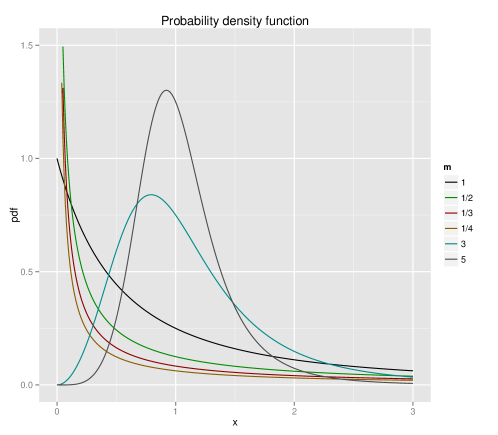
Figure 1: Pdf of the Lavalette distribution. Some Lavalette probability density functions (Eq.(4) with identical parameter $C=1$ but with a=1/5, 1/3, 1, 2, 3, and 4 ($m=1/a=1/b$).

Resemblance between Lavalette and lognormal distributions

To examine which well known pdf’s share the same property of $a=b$ when fitted to the DGBD rank function, we generated data from 14 distributions (beta, binomial, $\chi^{2}$, exponential, gamma, geometric, hypergeometric, lognormal, Mandelbrot, negative binomial, Pareto, Poisson, uniform and Weibull), and fit the ranked data by the Beta rank function via linear regression of the logarithmic transformation of Eq.(1). The estimated parameter values for $a$ and $b$ are shown in Fig.2. Interestingly, the only known pdf which exhibits $a\approx b$ is the lognormal distribution.

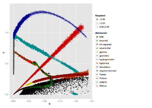
Figure 2: DGBD fits for various distributions. The estimated $a$ and $b$ parameter values in DGBD (Eq.(1)) for data generated by well known distributions. Size of the dots indicate the coefficient of determination R squared. The dots around the $a=b$ diagonal line are for data generated by the lognormal distribution.

We use a novel argument from statistics to explain why the Lavalette and lognormal distributions may be difficult to distinguish within a certain interval of their domain. There are two models for probability of a binary variable $y\in(0,1)$: (i) probit model Bliss (1934): $P=P(y=1)=\Phi(z)$ where $\Phi$ is the cdf of standard normal distribution; (2) logit model or logistic regression McCullagh and Nelder (1989): $P=1/(1+e^{-z})$. The two regression models for binary variable (regressed over an independent variable $z$) usually lead to similar results Aldrich and Nelson (1984); Agresti (2013), which can be written as (after the logistic variable being re-scaled by a factor $\alpha$):

$$\Phi(z)\approx\frac{1}{1+e^{-\alpha z}},\hskip 7.22743pt{\mbox{o}r,}\hskip 7.22743pt\frac{\Phi(z)}{1-\Phi(z)}\approx e^{\alpha z}.$$ (6)

The $\alpha$ can be $\sqrt{8/\pi}\approx 1.596$ to achieve the best fit near the midpoint Page (1977), or $\approx 1.7$ to best fit the whole range, or $\pi/\sqrt{3}\approx 1.81$ which is the standard deviation of the variable from the logistic distribution Agresti (2013). The standard normal variable can be converted to a lognormal distribution variable $x$: $z=(\log(x)-\mu)/\sigma$, and re-expressing Eq.(6) in $x$ becomes:

$$e^{\mu}\left(\frac{\Phi((\log(x)-\mu)/\sigma}{1-\Phi((\log(x)-\mu)/\sigma)}\right)^{\sigma/\alpha}\approx x,$$ (7)

which we recognize as the Lavalette rank function over variable $x$ ($1-\Phi$ is the normalized rank). This derivation also points out that the parameter $a=b$ is the standard deviation of the lognormal distribution divided by $\alpha(=1.6\sim 1.8)$, whereas the log-mean of the lognormal distribution is related to the scaling parameter by $C=e^{\mu}$. Since probit and logistic regression are not the same, we conclude that the Lavalette and the lognormal distributions cannot be identical. Indeed, the Lavalette and lognormal distributions have qualitatively different behaviours at the tails. All moments of the lognormal distribution exist, while the Lavalette has only finite moments of order $i<1/a$, as we previously discussed. If there is enough data to sample the tail, they cannot be mistaken into one another.

Fig.3 illustrates directly the similarity between the Lavalette and lognormal distributions. The cdf’s of lognormal distribution and the corresponding Lavalette distribution are plotted at three different parameter values ($\mu=0$ with $\sigma=0.1,\,0.5$ and $1$ for the lognormal, corresponding $C=e^{\mu},\,a=\sigma\sqrt{3}/\pi$ for the Lavalette). Besides the difference at the tails (which is not visible from the cdf plot because the difference along the $y$-axis is very small for extreme values), the two functions also deviate slightly from each other in the middle range. This deviation is equivalent, after a transformation, to that between the cdf of standard normal distribution and logistic function. It has been proposed that a modification of the logistic function, $1/(1+exp(-1.5876x-0.070566x^{3}))$, is a very good approximation of the cdf of standard normal distribution Johnson et al. (1994); Page (1977). The small coefficient of the high-order term is another indication that the cdf of normal and logistic function, or equivalently, lognormal and Lavalette distributions, are close.

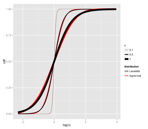
Figure 3: Lognormal vs Lavalette cdf. Cumulative distribution function for lognormal and Lavalette distributions, being $\mu=0$ and $\sigma=0.1,\,0.5$ and $1$ the parameters of the lognormal. The $x$ axis is in logarithmic scale. We see that over an important interval of the domain, it may be difficult to distinguish a lognormal from a Lavalette distribution.

Occurrence and Applications

To illustrate that Lavalette distribution can be applied to real data, we examine several datasets besides the impact factor and citation data used in Lavalette (1996); Popescu (1997). We will give examples of population data, amino acid mutation rates and codon usage data where the Lavalette distribution is a good statistical model. The parameters were estimated through linear regression of the logarithmic transformation of Eq.(1), which in our case gives very similar results to maximum likelihood estimators. The goodness of fit tests were performed using the Kolmogorov-Smirnov statistic and the $p-$values were estimated through a Monte-Carlo approach proposed in (Clauset et al. (2009)). As usual, a small $p-$ value leads to reject the hypothesis that the data are well described by a Lavalette distribution.

The first set of examples is about administrative units of population. Most countries in the world are internally divided into administrative units, which may be called states, provinces, etc. Law (1999). We call these primary administrative units (PAU), which may be in turn subdivided into smaller or second level administrative units (counties, municipalities, etc.) We call these secondary administrative units (SAU). In the same way, there may be third level units (TAU) and so forth. We give three examples of occurrence of the Lavalette distribution: the Nigeria (NRG) population of local government areas (SAU) and the municipality population (TAU), below province and autonomous community, within the Spanish provinces of Madrid and Cádiz. We chose these examples after analysing population data from many countries in the world and picking those that are best fitted by the Lavalette function. We emphasize that we do not claim the Lavalette distribution to be ubiquitous in any way; our purpose is to show that there are some datasets where it can be a good statistical model.

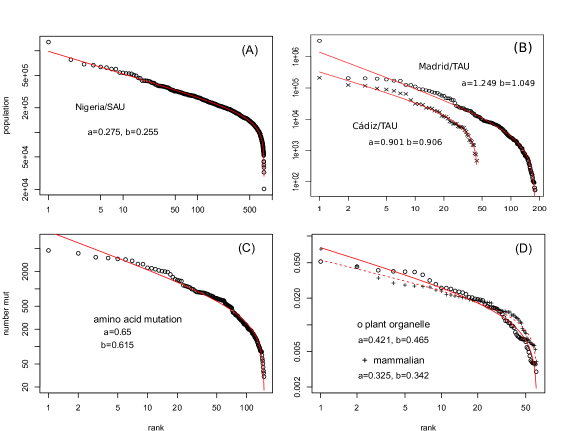
Figure 4: Ranked datasets fitted by Lavalette rank function. (A) Nigeria (NRG) local government area (the secondary administrative unit (SAU)) population; (B) Madrid and Cádiz municipality (the tertiary administrative unit (TAU)) population; (C) Amino acid to amino acid mutation counts in the 1000 Genomes Project; (D) Averaged codon usage (excluding the three stop codons) of plant organelles and mammals.

Fig.4(A,B) shows the rank frequency distribution of the NRG/SAU, Madrid/TAU and Cádiz/TAU population in log-log scale. The fitted parameter values $(a,b)$ by Eq.(1) are (0.275, 0.255) for NRG/SAU, (1.249, 1.049) for Madrid/TAU, (0.901, 0.906) for Cádiz/TAU, all with $a\approx b$. Clearly these do not follow a power law distribution. Although city population is one of the well known examples of Zipf’s law Krugman (1996); Jiang and Jia (2010), there is a difference between cities and administrative units. The origin of Zipf’s law in population and economic phenomena might be explained by a proportionate-growth random process Gabaix (1999). For the particular case of well separated cities, as well as firm sizes, birth and death processes explain the origin and robustness of Zipf’s law Saichev et al. (2010). However, when regions are artificially partitioned, such as the case of administrative units, the argument for power-law may fail. Indeed, the bad fitting performance of Zipf’s law on data in some counties Soo (2005); Rozenfeld et al. (2011) might be caused by the artificial boundary in defining a city Holmes and Lee (2010). This leaves room for alternative functional form such as DGBD. Martínez-Mekler et al. (2009).

The second example is the amino acid mutation rates de Beer et al. (2013) based on the amino acid changing (missense) variants in the 1000 Genomes Project 1000 Genomes Project Consortium et al. (2010). A missense mutation is a point mutation which results in the codification of a different amino acid. Because the variants are observed in normal human population with a short evolutionary history, it can be considered as an instantaneous mutation rate. The substitution rate between different species, such as the point accepted mutation (PAM) Dayhoff et al. (1978), cover a much longer evolutionary history with stronger selection constraints. Out of 380 ( = 20 $\times$ 19) possible mutations between 20 amino acids, only $N=$ 150 are allowed from the single base mutation in the DNA sequence, due to the nature of the genetic code. Fig.4(C) shows the ranked amino acid to amino acid frequencies derived from the missense variants in DNA sequence of the 1000 Genomes Project. Fig.4(C) shows a fitting by the Beta rank function Eq.(1) with $a\approx 0.650$ and $b\approx 0.615$, which is again a good Lavalette function.

The third example is the codon usage of $N=$ 61 non-stop codons, with data from the Codon Usage Database Nakamura et al. (2000). Codon usage refers to the frequency of occurrence of 181 each type of codon within a DNA sequence. We picked the two examples best demonstrating Lavalette function: genes in plant organelles (9221 species) and in (non-primate, non-rodent) mammalian nucleus (433 species). The codon frequencies are averaged over all species in plant organelle and mammalian separately. The three stop codons are discarded. The $(a,b)$ are (0.422, 0.465) for plant organelles, and (0.325,0.342) for mammalian (Fig.4(D)).

With the previous examples we have illustrated the occurrence of the Lavalette distribution. Next we propose a statistical criterion to discern if this distribution is consistent with the data.

Goodness of Fit Tests

The first clue that a certain dataset may be well described by the Lavalette distribution is to fit the data to DGBD function Eq.(1), estimate the parameters and check if $a\approx b$. If this is the case, the data set is a candidate for the Lavalette distribution. This is a first criterion and it serves to rule out many datasets; however, it is by no means strong statistical evidence to claim the the Lavalette is a good model for the data.

To test more rigorously whether a Lavalette function fits the observed data well, we use a re-sampling approach as discussed in Clauset et al. (2009) which can also be called a bootstrap Efron and Tibshirani (1993). We first fit the data by the Lavalette function (Eq.(2)). The difference between the observed and fitted value is measured by the Kolmogorov-Smirnov (KS) distance. Using the fitted Lavalette rank function, artificial data (replicates) are generated multiple times: each time a new Lavalette rank function is fitted and KS distance calculated. The proportion of replicates with larger KS distances than the observed one is the empirical $p$-value.

A large empirical $p$-value indicates that there is not enough evidence to reject the Lavalette function. Empirical $p$-values from 1000 replicates are 0.49 for NRG/SAU, 0.91 for Madrid/TAU, 0.88 for Cádiz/TAU, 0.06 for mutation rate, and 0.4 for codon usage in both plant organelle and mammals. These values depend on many specific choices used, e.g. how to handle replicates which have the same KS distance as the observed one, using KS distance instead of some other measure of difference between two curves, the number of replicates, etc. The empirical $p$-value we have indicate that Eq.(2) is a good fitting function for these data.

There have been debates in the literature whether Zipf’s law results from the central limit theorem Perline (1996); Troll and P Beim Graben (1998); Mitzenmacher (2004). Given a dataset, the best answer to that debate is to pick the better fitting model between power law and lognormal distribution Malevergne et al. (2011). The approximate equivalence between Lavalette distribution and lognormal distribution provides us with a simple method in deciding if a set of data follows Zipf’s law or lognormal distribution. For the fitting of ranked data by the Beta rank function Eq.(1), if $b\approx 0$, the Zipf’s law is better; if $a\approx b>0$, lognormal is better; and if $a\neq b\gg 0$, neither are good fitting functions.

For our examples to illustrate the Lavalette distribution in real data, it is obvious that lognormal distribution is a better fitting function than the Zipf’s law. We can further quantify the fitting performance by model selection techniques such as Akaike information criterion (AIC) Burnham and Anderson (2003); Akaike (1974); Li (2001), with the better model exhibiting lower AIC value. The AIC_lav-AIC_zipf= $N\log(SSE_{lav}/SSE_{zipf})$ Li and Miramontes (2011), where SSE is the sum squared error, is -3284.6,-410.3, -108.1 for the NRG/SAU, Madrid/TAU, Cádiz/TAU data, -353.7 for the amino acid mutate data, and -101.7, -114.7 for plant organelle, mammalian codon frequencies, all representing an overwhelming support to the Lavalette function or lognormal distribution over the Zipf’s law.

Discussion and Conclusions

We have presented a novel probability distribution function and showed that it is a good alternative for data that does not follow a perfect Zipf’s law. We have seen that this distribution yields a very good approximation to the lognormal distribution. Although it is perhaps less important because of the approximate equivalence between the Lavalette and the lognormal distributions, one may still sometimes want to determine whether a data is better fitted by the Lavalette or lognormal distribution. We propose the following procedure for this test: (i) log-transform, then standardize (zero mean, unit standard deviation) the raw data, to $x^{\prime}$; (ii) compare the empirical cdf of $x^{\prime}$ to both standard normal and logistic distribution cdf with a scaling parameter $\alpha=\pi/\sqrt{3}$ ($cdf=1/(1+e^{-\alpha x^{\prime}})$); (iii) if the standard normal function is closer to the data, lognormal distribution fits the original data better, otherwise, Lavalette function is better. Using this procedure and KS distance as the measure of difference, NRG/SAU is the only data which Lavalette is better than lognormal distribution. If sum of absolute error is used to measure the difference, codon usage of mammals is another data which prefers Lavalette over lognormal.

In conclusion, by connecting Lavalette function to lognormal distribution, we achieve a better understanding of the DGBD function and the limitations of the Zipf’s law.

Materials and Methods

Population data for administrative units and sub-units in a large sample of countries is available in the database Statoids http://www.statoids.com (accessed April 2016). Population of local government areas (SAU) in Nigeria were taken from this database. Spain’s population at PAU, SAU and TAU levels are available from the National Statistics Institute (INE), http://www.ine.es/en/pob_xls/pobmun12_en.xls. We chose these examples after analysing population data from many countries in the world and picking those that are best fitted by the Lavalette function.

Amino acid to amino acid mutation rates were calculated from missense variants, taken from DNA sequence of the 1000 genomes project, available at http://www.1000genomes.org/. In particular, we used mutation data from http://journals.plos.org/ploscompbiol/article?id=10.1371/journal.pcbi.1003382 fig (1). From this data, we counted the relative frequency of occurrence for each mutation.

We calculated codon usage of 61 non-stop codons for genes in plant organelles and non-primate and non-rodent mammalian nucleus. Data were downloaded from Codon Usage Database http://www.kazusa.or.jp/codon/.

All the data used in our analysis is available on https://figshare.com/articles/Data_rar/3363961.

Author Contributions

Conceived and designed the experiments OF PM GC WL. Performed the experiments OF WL. Analysed the data OF YY WL. Wrote the paper OF WL.

References

- Clauset et al. (2009) A. Clauset, C. Shalizi, and M. Newman, SIAM Rev. 51, 661 (2009).
- Sornette (2006) D. Sornette, Critical Phenomena in Natural Sciences, 2nd ed. (Springer-Verlag, Berlin, 2006).
- Zipf (1935) G. Zipf, The Psycho-Biology of Languages (Houghtion-Mifflin, Boston, MA, 1935).
- Gabaix (1999) X. Gabaix, Am. Econ. Rev. 89, 129 (1999).
- Gopikrishnan et al. (1999) P. Gopikrishnan, V. Plerou, L. Amaral, M. Meyer, and E. Stanley, Phys Rev E 60, 5305 (1999).
- Axtell (2001) R. Axtell, Science 293, 1818 (2001).
- Petersen et al. (2011) A. Petersen, H. Eugene, and S. Succi, Sci. Rep. 1, 181 (2011).
- Petersen and Succi (2013) A. Petersen and S. Succi, Journal of Informetrics 7, 823 (2013).
- Li (2002) W. Li, Glottometrics 5, 14 (2002).
- Stumpf and Porter (2012) M. Stumpf and M. Porter, Science 335, 665 (2012).
- Laherre and Sornette (1998) J. Laherre and D. Sornette, Eur. Phys. J. B. 2, 525 (1998).
- Bowman and Shenton (2007) K. Bowman and L. Shenton, Far East J. Theo. Stat. 23, 133 (2007).
- Mansilla et al. (2007) R. Mansilla, E. Köppen, G. Cocho, and P. Miramontes, J. Informetrics 1, 155 (2007).
- Martínez-Mekler et al. (2009) G. Martínez-Mekler, R. Martínez, M. B. del Río, R. Mansilla, P. Miramontes, and G. Cocho, PLoS ONE 4, e4791 (2009).
- Li and Miramontes (2011) W. Li and P. Miramontes, J. Quant. Ling. 18, 337 (2011).
- Li (1991) W. Li, Phy. Rev. A 43, 5240 (1991).
- Alvarez-Martinez et al. (2011) R. Alvarez-Martinez, G. Martinez-Mekler, and G. Cocho, Physica A 390, 120 (2011).
- Li et al. (2010) W. Li, P. Miramontes, and G. Cocho, Entropy 12, 1743 (2010).
- del Río et al. (2008) M. B. del Río, G. Cocho, and G. Naumis, Physica A 387, 5552 (2008).
- Li (2012a) W. Li, Physica A 391, 49 (2012a).
- Li (2012b) W. Li, Complexity 18, 44 (2012b).
- Li (2013) W. Li, J. Quant. Ling. 20, 153 (2013).
- Li et al. (2014) W. Li, J. Freudenberg, and P. Miramontes, BMC Bioinfo. 15, 2 (2014).
- Ausloos (2014) M. Ausloos, Phys. Rev. E 89, 062803 (2014).
- Newman (2005) M. E. J. Newman, Contemporary Physics 46, 323 (2005).
- Lavalette (1996) D. Lavalette, INSERM preprint U350 (1996).
- Popescu (1997) I. Popescu, Romanian Rep. Phys. 49 (1997).
- Popescu (2003) I. Popescu, Glottometrics 6, 83 (2003).
- Lavalette (2007) D. Lavalette, in Exact Methods in the Study of Language and Text, edited by P. Grzybek and R. Köhler (Mouton de Gruyter, Berlin, Boston, 2007) pp. 371–382.
- Voloshynovska (2011) I. Voloshynovska, J. Quant. Ling. 18, 274 (2011).
- Gradshteyn and Ryzhik (2007) I. Gradshteyn and I. Ryzhik, Table of Integrals, Series, and Products, seventh ed. (Academic Press, Burlington, MA, USA, 2007).
- Bliss (1934) C. Bliss, Science 79, 38 (1934).
- McCullagh and Nelder (1989) P. McCullagh and J. Nelder, Generalized Linear Models, 2nd ed. (Chapman and Hall/CRC, London, 1989).
- Aldrich and Nelson (1984) J. Aldrich and F. Nelson, Linear Probability, Logit, and Probit Models, 1st ed. (Sage Pub., Newbury Park, CA, USA, 1984).
- Agresti (2013) A. Agresti, Categorical Data Analysis, 3rd ed. (Wiley, Hoboken, NJ, USA, 2013).
- Page (1977) E. Page, Appl. Stat. 26, 75 (1977).
- Johnson et al. (1994) N. Johnson, S. Kotz, and N. Balakrishnan, Continuous Univariate Distributions, 2nd ed. (John Wiley & Sons, New York, USA, 1994).
- Law (1999) G. Law, Administrative Subdivisions of Countries: A Comprehensive World Reference, 1900 through 1998, 1st ed. (McFarland & Co., Jefferson, NC, USA, 1999).
- Krugman (1996) P. Krugman, The Self-Organizing Economy (Blackwell, Cambridge, MA, USA, 1996).
- Jiang and Jia (2010) B. Jiang and T. Jia, Int. J. Geograph. Info. Sci. 25, 1269 (2010).
- Saichev et al. (2010) A. Saichev, Y. Malevergne, and D. Sornette, Theory of Zipf’s law and beyond (Springer Verlag, 2010).
- Soo (2005) K. Soo, Reg. Sci. Urb. Econ. 35, 239 (2005).
- Rozenfeld et al. (2011) H. Rozenfeld, D. Rybski, X. Gabaix, and H. Makse, Am. Eco. Rev. 101, 2205 (2011).
- Holmes and Lee (2010) T. Holmes and S. Lee, in Agglomeration Economics, edited by E. Glaeser (Univ. Chicago Press, Chicago, IL, USA, 2010) pp. 105–131.
- de Beer et al. (2013) T. de Beer, R. Laskowski, S. Parks, B. Sipos, N. Goldman, and J. Thornton, PLoS Genet. 9, e1003382 (2013).
- 1000 Genomes Project Consortium et al. (2010) 1000 Genomes Project Consortium, R. Durbin, G. Abecasis, D. Altschuler, A. Auton, and et al., Nature 467, 1061 (2010).
- Dayhoff et al. (1978) M. Dayhoff, R. Schwartz, and B. Orcutt, in Atlas of Protein Sequence and Structure, edited by M. Dayhoff (Natl. Biomed. Res. Found., Washington, DC, USA, 1978) pp. 345–362.
- Nakamura et al. (2000) Y. Nakamura, T. Gojobori, and T. Ikemura, Nucl. Acids Res. 28, 292 (2000).
- Efron and Tibshirani (1993) B. Efron and R. Tibshirani, An Introduction to the Bootstrap (Chapman & Hall, London, UK, 1993).
- Perline (1996) R. Perline, Phys. Rev. E 54, 220 (1996).
- Troll and P Beim Graben (1998) G. Troll and P Beim Graben, Phys. Rev. E 57, 1347 (1998).
- Mitzenmacher (2004) M. Mitzenmacher, Internet Math. 1, 226 (2004).
- Malevergne et al. (2011) Y. Malevergne, V. Pisarenko, and D. Sornette, Phys. Rev. E 83, 036111 (2011).
- Burnham and Anderson (2003) K. Burnham and D. Anderson, Model Selection and Multi-Model Inference, 2nd ed. (Springer-Verlag, New York, USA, 2003).
- Akaike (1974) H. Akaike, IEEE Trans. Automatic Control 19, 716 (1974).
- Li (2001) W. Li, Phys. Rev. Lett. 86, 5815 (2001).