Analysis of the $e^{+}e^{-}\rightarrow\pi^{0}\gamma$ process using anomaly sum rules approach

Abstract

The process $e^{+}e^{-}\rightarrow\gamma^{*}\rightarrow\pi^{0}\gamma$ was considered using time-like pion transition form factor, obtained in the approach of the Anomaly Sum Rules(ASR). The total cross section and angular distribution of the process was calculated. As the result of the comparison with the data it was shown that ASR approach provides their good description in the regions far from the pole. Also there was proposed a method allowing to give reasonable description of data in the region of pole within the ASR approach. The strong restrictions for the parameters of the modified ASR approach were obtained.

1 Introduction

The transition form factor(TFF) of the pion is attracting the great interest last years. In particular, it is related to the pion radius at small virtualities of the photon. It is used for description of the hadrons-photon interactions, and within it, it is possible to match predictions of the pQCD and non-perturbation methods.

The space-like region of the transition form factor of the $\pi^{0}$ is quite good investigated. The available experimental data cover a fairly wide range of $Q^{2}$. The CELLO[1] and CLEO[2] collaborations measured it in the intervals $0.7-2.2\ GeV^{2}$ and $1.6-8.0\ GeV^{2}$ , respectively. The BaBar[3] and Belle[4] move the range of $Q^{2}$ up to 40 $GeV^{2}$. At the $1.0\leq Q^{2}\leq 9$ all the experiments show same behaviour and agree with theoretical expectations[5]. From the other side, there is well known contradiction between BaBar[3] and Belle[4] results of the measurement of the $\pi^{0}$ TFF at the region of the large space-like photon virtualities. At the same time, in the region of low $Q^{2}$ and in the time-like region the number of direct measurements of the pion TFF is quite small. The more precise data are expected in the future from BES-III[6] and KLOE-2[7] collaborations.

Our paper is dedicated to the pion transition form factor in the time-like region. In this region pion TFF can be studied in the process $e^{+}e^{-}\rightarrow\gamma^{*}\rightarrow\pi^{0}\gamma$. The SND[8] (the most accurate data on the process $e^{+}e^{-}\rightarrow\pi^{0}\gamma$ to date) and CMD2[9] experiments had collected the data that cover the range $0.6-1.38\ GeV$ of $\sqrt{s}$. Theoretically, the process was studied in the work [10], with using the methods of the dispersive theory. In the future, CLAS[11] will provide more precise data of the direct measurements of the time-like pion TFF.

Recently a new method was offered to describe the pion form factor based on the dispersive representation of the axial anomaly [12],[13] (see also review [14]). This method has an advantage of being model-independent and not relying on the QCD factorization. Also in this approach the pion TFF can be described in the whole region of the photon virtualities $Q^{2}=-q^{2}$. In the paper [13] the pion TFF was obtained in the whole space-like region $Q^{2}>0$. Later it was analytically continued to the time-like region [15]. As soon as this method is based on the exact relation, implied by the axial anomaly it provides very powerful tool to study pion (and other pseudoscalar mesons) TFFs both in space-like and time-like regions.

The goal of this work is to check predictions of the ASR method in the time-like region at low $q^{2}$ using the SND and CMD2 experimental data.

The paper is organized as follows: the section 2 contains a brief description of the main steps of the pion TFF calculation and the calculation of total cross section and angular distribution of the process $e^{+}e^{-}\rightarrow\gamma^{*}\rightarrow\pi^{0}\gamma$; in the next section 3 the obtained expressions are compared with the experimental data: the subsection 3.1 comprises analysis of the situation far from the poles, while the subsections 3.2 and 3.3 are dedicated to the attempts to find modifications to the expression of the pion TFF in order to describe data peaks, within the ASR approach; in the last section 4 we summarize the obtained results.

2 Total cross section calculation

Let us consider a process $e^{+}e^{-}\rightarrow\gamma^{*}\rightarrow\pi^{0}\gamma$. It can be expressed in terms of the pion TFF $F(q^{2})$, which is defined as:

$$\int d^{4}xe^{ikx}\langle\pi^{0}(p)|T\{J_{\mu}(x)J_{\nu}(0)\}|0\rangle=\epsilon_{\mu\nu\rho\sigma}k^{\rho}q^{\sigma}F(q^{2})\;,$$ (1)

where $k,q$ are momenta of photons, $p=q-k$, and two electromagnetic currents $J_{\mu}=\sum\limits_{i=u,d,s}e_{i}\bar{q_{i}}\gamma_{\mu}q_{i}$. In what following all the expressions will be written in the unit of electron charge $|e|=1$, while in the equations for cross sections and amplitudes explicit dependence of electron charge is restored. One photon is real $(k^{2}=0)$ and the other one is virtual. The Feynman diagram is shown on the Fig.1.

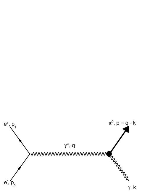
Figure 1: Feynman diagram of the process.

The expression for the pion TFF was obtained in approach based on the dispersive representation of the axial anomaly in the works [13],[15]. Here we briefly recall the main steps of the method.

The vector-vector-axial triangle graph amplitude, where the axial anomaly occurs, contains an axial current $J_{\alpha 5}$ and two electromagnetic currents $J_{\mu}=\sum\limits_{i=u,d,s}e_{i}\bar{q_{i}}\gamma_{\mu}q_{i}$,

$$T_{\alpha\mu\nu}(k,q)=\int d^{4}xd^{4}ye^{(ikx+iqy)}\langle 0|T\{J_{\alpha 5}(0)J_{\mu}(x)J_{\nu}(y)\}|0\rangle,$$ (2)

where $k$ and $q$ are the photons momenta. In what follows, we limit ourselves to the case when one of the photons is on-shell ($k^{2}=0$). As it was shown in the paper [12] the imaginary part $A_{3}$ of the of the invariant amplitude at the tensor structure $k_{\nu}\varepsilon_{\alpha\mu\rho\sigma}k^{\rho}q^{\sigma}$ in the variable $(k+q)^{2}=s>0$ satisfy the following relation:

$$\int_{0}^{\infty}A_{3}(s,q^{2};m_{i}^{2})ds=\frac{1}{2\pi}\frac{1}{\sqrt{2}}.$$ (3)

The relation (3) is exact: $\alpha_{s}$ corrections are zero and it is expected that all nonperturbative corrections are absent as well (due to ’t Hooft’s principle [12, 16]). Note, in the original paper [12] the eq.(3) was obtained for the space-like photon $(q^{2}<0)$. Later in the paper [15] analytical continuation to the time-like region was developed.

Supposing that $A_{3}$ decreases fast enough at $\lvert q^{2}\rvert\to\infty$ and is analytical everywhere except the cut $q^{2}\in(0,+\infty)$, it was found

$$p.v.\int_{0}^{\infty}ds\int_{0}^{\infty}dy\frac{\rho(s,y)}{y-q^{2}}=\frac{1}{\sqrt{2}},$$ (4)

$$\int_{0}^{\infty}ds\rho(s,q^{2})=0,\;.$$ (5)

where $\rho=2Im_{q^{2}}A_{3}$. Saturating the lhs of the three-point correlation function (2) with the resonances in the axial channel, singling out the first (pion) contribution and replacing the higher resonance’s contributions with the integral of the spectral density, the ASR in the time-like region (4) leads to

$$\pi f_{\pi}ReF_{\pi\gamma}(q^{2})+\int_{s_{3}}^{\infty}A_{3}(s,q^{2})ds=\frac{1}{2\pi}\frac{1}{\sqrt{2}},$$ (6)

where $s_{3}$ is duality region of the pion in the isovector channel, the definition of the TFFs $F_{\pi\gamma}$ is (1), and the meson decay constant $f_{\pi}$ is,

$$\langle 0|J_{\alpha 5}(0)|\pi^{0}(p)\rangle=ip_{\alpha}f_{\pi},$$ (7)

where $J_{\alpha 5}(0)=\frac{1}{\sqrt{2}}(\bar{u}\gamma_{\alpha}\gamma_{5}u-\bar{d}\gamma_{\alpha}\gamma_{5}d)$. As the integral of $A_{3}$ in eq.(6) is over the region $s>s_{3}$, we expect that nonperturbative corrections to $A_{3}$ in this region are small enough and we can use the one-loop expression for it.

Then the ASR leads to the pion TFF:

$$F(q^{2})=\frac{1}{2\sqrt{2}\pi^{2}f_{\pi}}\frac{s_{3}}{s_{3}-q^{2}}.$$ (8)

As were discussed in the papers [13],[15], this result is valid in both time-like and space-like regions (expect the pole $q^{2}=s_{3}$).

The numerical value of $s_{3}$ was obtained in the limit $-q^{2}\rightarrow\infty$ of the space-like ASR [13], $s_{3}=4\pi^{2}f^{2}_{\pi}=0.67\ GeV^{2}\pm 10\%$. This expression coincides with the one obtained earlier from the two-point correlator analysis[17] and is close to the numerical value obtained from two-point sum rules[18]. In the recent analysis light cone and anomaly sum rules predictions were compared [19], and it was shown that $s_{3}$ is indeed approximately constant with the accuracy about $\pm 10\%$. At same time it was noted that in the region of small $q^{2}$ the value $s_{3}=0.61\ GeV^{2}$ is more preferable.

As we can see from (8) the pion time-like TFF has a pole at $q^{2}=s_{3}$, which is numerically close to $m^{2}_{\rho}\approx 0.6\ GeV^{2}$ and to $m_{\omega}^{2}\approx 0.61\ GeV^{2}$. The pole behavior (which corresponds to zero width of the ρ meson) appeared since we used the one-loop approximation for $A_{3}$, neglecting the possible dependence of $s$ on $Q^{2}$ and final-state interactions. Therefore, the eq. (8) can be used not too close to the pole $q^{2}=s_{3}$. The effect of the finite width can be estimated if one takes into account small corrections: as perturbative($\alpha_{s}^{2}$ and higher) as non-perturbative; and also the small effects of mixing.

One can write down the amplitude $M_{\pi\gamma}$ as:

$$M_{\pi\gamma}=ie^{3}\bar{u}\gamma^{\alpha}u\frac{g_{\alpha}^{\mu}}{q^{2}}\epsilon_{\mu\nu\rho\sigma}k^{\rho}q^{\sigma}F(q^{2})(e^{\nu})^{*}$$ (9)

Neglecting masses and summing over polarisations, the square of the amplitude takes form:

$$|M_{\pi\gamma}|^{2}=\frac{e^{6}}{4}Sp[\not{p_{1}}\gamma^{\mu}\epsilon_{\mu\nu\rho\sigma}k^{\rho}q^{\sigma}\not{p_{2}}\gamma^{\mu^{\prime}}\epsilon_{\mu^{\prime}\nu^{\prime}\rho^{\prime}\sigma^{\prime}}k^{\rho^{\prime}}q^{\sigma^{\prime}}g^{\nu\nu^{\prime}}]\frac{|F^{2}(q^{2})|}{q^{4}}.$$ (10)

Total cross section has the form:

$$\sigma=\frac{2}{3}\pi^{2}\alpha_{QED}^{3}|F^{2}(q^{2})|.$$ (11)

Finally, substituting eq.(8) to (11) we obtain expression for the total cross section:

$$\sigma_{theor}=\frac{\alpha_{QED}^{3}}{12\pi^{2}f_{\pi}^{2}}\frac{s_{3}^{2}}{(s_{3}-q^{2})^{2}}.$$ (12)

And the expression for angular distribution has a rather common form implied by angular momentum conservation:

$$\frac{d\sigma}{d\cos\theta}\big{|}_{\pi}^{0}=\frac{\alpha_{QED}^{3}}{32\pi^{2}f_{\pi}^{2}}\frac{s_{3}^{2}}{(s_{3}-q^{2})^{2}}(1+\cos^{2}\theta).$$ (13)

3 Comparison with data

3.1 Comparison with experiment out of poles

In this section we will compare theoretical results of the ASR approach (12) with SND2016 and CMD2 experimental data [8],[9]. The curves corresponding to eq.(12) with the lower and upper limits $s_{3}=0.61,0.67\ GeV^{2}$ are shown (by the dashed and solid lines) on the Fig.2.

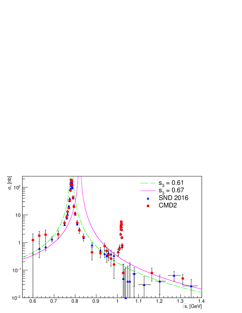
Figure 2: Total cross section $\sigma_{theor}$ vs. SND2016 and CMD2 [8, 9] data.

Let us emphasize, that the eq.(8) indicates the $\rho-\omega$ meson resonance( in the zero width approximation) position, but do not indicate the existence of the second resonance, corresponding to the $\phi$ meson mass. The reason of this is that the equation of the pion TFF was obtained for the isovector channel of the axial current and it does not take into account the possible effects of mixing. So the hadrons including s-quarks can’t be accounted in such approximation. Discussion and possible treatment of this will be done later in the next sections.

Note, that from the Fig.2 one can see curve with $s_{3}=0.67\ GeV^{2}$(solid line) describes data much worse, than with $s_{3}=0.61\ GeV^{2}$(dashed line). This one coincides with the results of the matching Light-Cone Sum Rules(LCSR) and ASR approaches[19] in the space-like region, where, as it was mentioned earlier, it was shown that at the region of small $q^{2}$ the value $s_{3}=0.61\ GeV^{2}$ is more preferable, while within the $\pm 10\%$ error of the $s_{3}$ calculation the value $s_{3}=0.67\ GeV^{2}$ also agrees with the experiment. But in the time-like region of the $q^{2}$, as can be seen from Fig.2, the equation for the pion TFF (8), and the corresponding total cross section (12), is much more sensitive to the value of the $s_{3}$, and the value $s_{3}=0.67\ GeV^{2}$ has much worse agreement with the experiment, than $s_{3}=0.61\ GeV^{2}$. Thus, the time-like region is a kind of a microscope for analysis of the parameters of the axial channel in the space-like region. So we can expect, that analysis of the pion TFF in the time-like region of $q^{2}$ allows to clarify the values of the small corrections, which one are hard to determine in the space-like region.

The fact that the pole of the eq.(12) $q^{2}=s_{3}=0.61$ is close to the $m_{\rho}^{2}\approx 0.60\ GeV^{2},m_{\omega}^{2}\approx 0.61\ GeV^{2}$ is quite interesting. It actually means that from the parameters of the axial channel one can obtain spectrum of masses in the vector channel. The tendency of $s_{3}$ variation in the space-like channel may be attributed to the effect of the pole in the time-like channel, requiring that

$$s(m_{V}^{2})=m_{V}^{2}.$$

Clearly, at present accuracy one cannot distinguish $\rho$ and $\omega$ masses.

It seems that more accurate analysis of the anomaly sum rule (4), which will takes into account the effects of $\pi,\eta,\eta^{\prime}$ mixings (as well as perturbative and non-perturbative small corrections), can provide a better description of the experimental data, in particular of the second peak on the Fig. 2. Theoretical estimations show, that if one includes the effects of the mixing into the calculation of the pion TFF, then one obtains more complicated expression than the eq.(8). It should be a linear combination of terms of the type of the eq.(8) and each of them will have its own value of $s_{3}$. This work is now in progress.

In the next chapter we discuss a modification of the eq.(8) in order to describe the peaks and estimate how good this approximation is be able to describe experimental data. Firstly, we consider the first peak and further generalize the result to the second one.

3.2 $\rho$-$\omega$ peak

Let us consider the first experimental peak, which one is corresponds to $\rho$-$\omega$ resonance. Here we perform fits of the data below $1.0\ GeV.$ The equation of the pion TFF (8) was obtained using zero width of $\rho$-meson, so the $ImF(q^{2})\sim\delta(s_{3}-q^{2})$. To get right description of the data, one should add to the denominator of (8) term, which should gives resonance corresponding to the data peak. It means that the $\rho$-meson should have finite width, so the $ImF(q^{2})$ will not have such a trivial form.

We modify (8) by adding to denominator the term of the form $im_{v}\Gamma_{v}$, so the equation for pion time-like TFF takes form similar to the relativistic Breit-Wigner amplitude:

$$F(q^{2})=\frac{1}{2\sqrt{2}\pi^{2}f_{\pi}}\frac{s_{3}}{s_{3}-q^{2}+im_{v}\Gamma_{v}}.$$ (14)

Substituting to (10) the modified pion TFF equation (14), with the values of the $m_{v},\Gamma_{v},s_{3}=m_{v}^{2}$ corresponding to the $\rho$ and $\omega$ mesons( we take the averaged one values of masses and widths of the $\rho$ , $\omega$ mesons from PDG [20]: $m_{\rho}=0.77526\ GeV,\Gamma_{\rho}=0.149\ GeV,m_{\omega}=0.78265\ GeV,\Gamma_{\omega}=0.00849\ GeV.$), and doing simple calculations, we obtain two fits for total cross sections:

$$\sigma_{fit-\rho,\omega}=\frac{\alpha_{QED}^{3}}{12\pi^{2}f_{\pi}^{2}}\frac{s_{3\rho,\omega}^{2}}{(s_{3\rho,\omega}-q^{2})^{2}+m_{\rho,\omega}^{2}\Gamma_{\rho,\omega}^{2}}.$$ (15)

Result is shown on Fig.3 for $\rho$ and $\omega$ cases (dotted and dot-dashed lines, correspondingly). It is clearly seen that both of this cases have poor description of the experimental data. The description is also not improved when the more complicated models of the single resonance are applied.

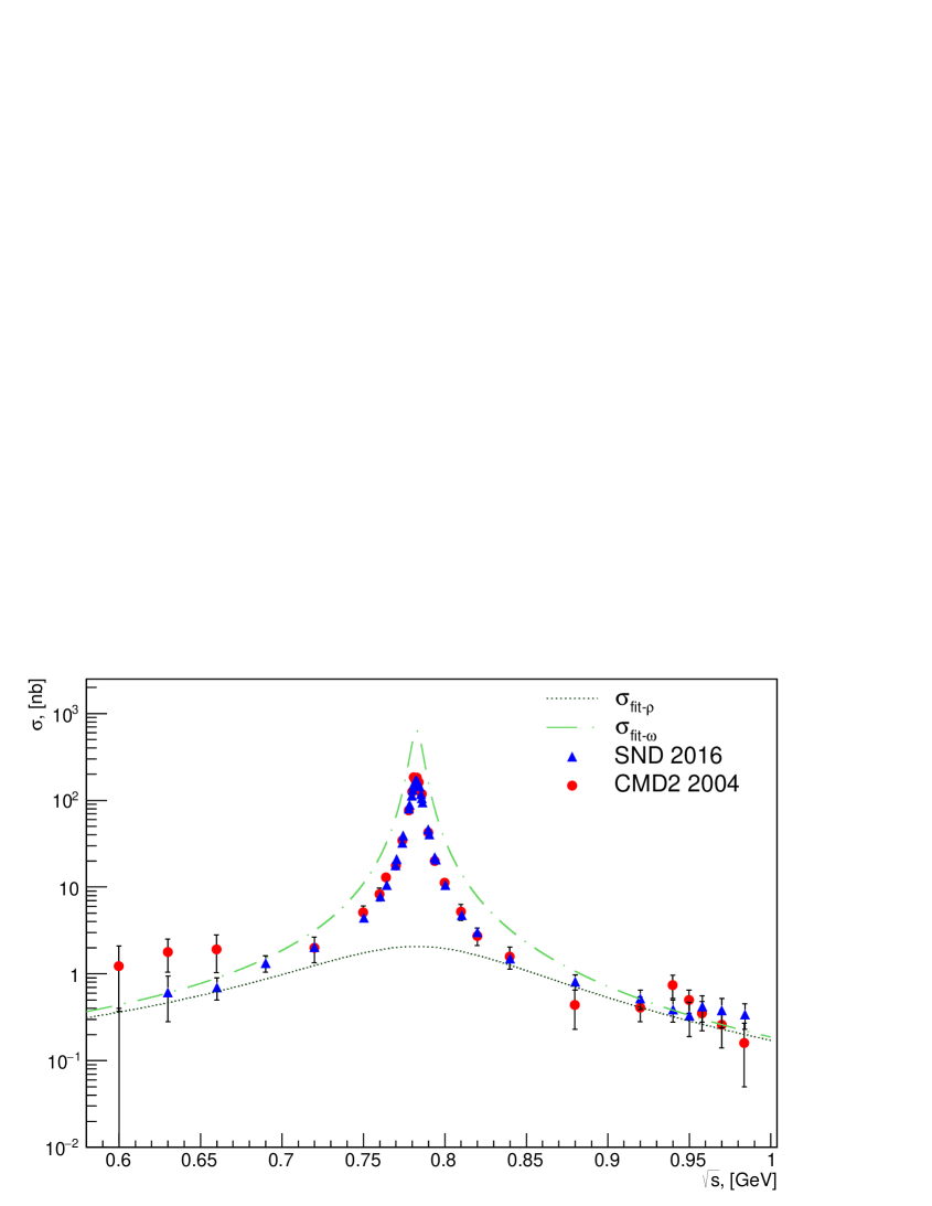
Figure 3: Fits of the $\rho-\omega$ peak with 1 resonance.

Thus we can assume, that reasonable description of the first experimental peak can be done by the to two resonance parametrisation. If one takes linear combination of amplitudes type of (14), so, that the pion TFF will be a sum of the two terms, where each one has the values of the $m_{v},\Gamma_{v},s_{3v}=m_{v}^{2}$ corresponding to the $\rho$ and $\omega$ mesons:

$$F(q^{2})=\frac{1}{2\sqrt{2}\pi^{2}f_{\pi}}\left(\alpha\frac{s_{3\rho}}{s_{3\rho}-q^{2}+im_{\rho}\Gamma_{\rho}}+\beta\frac{s_{3\omega}}{s_{3\omega}-q^{2}+im_{\omega}\Gamma_{\omega}}\right).$$ (16)

Then total cross section takes form:

$$\sigma_{fit-2resonances} = \frac{\alpha_{QED}^{3}}{12\pi^{2}f_{\pi}^{2}}\Big{(}\alpha^{2}\frac{s^{2}_{3\rho}}{(s_{3\rho}-q^{2})^{2}+m_{\rho}^{2}\Gamma_{\rho}^{2}}+\beta^{2}\frac{s^{2}_{3\omega}}{(s_{3\omega}-q^{2})^{2}+m_{\omega}^{2}\Gamma_{\omega}^{2}}+{}$$ (17)

$$+2\alpha\beta s_{3\rho}s_{3\omega}\frac{(s_{3\rho}-q^{2})(s_{3\omega}-q^{2})+m_{\rho}\Gamma_{\rho}m_{\omega}\Gamma_{\omega}}{((s_{3\rho}-q^{2})^{2}+m_{\rho}^{2}\Gamma_{\rho}^{2})((s_{3\omega}-q^{2})^{2}+m_{\omega}^{2}\Gamma^{2}_{\omega})}\Big{)}.$$

Note, due to that far the pole one should obtain formula (8), so $\alpha+\beta\approx 1$.

The result is shown on the Fig.4(solid line), the values of the fit parameters are: $\alpha=0.52,\ \beta=0.49;$ and the values of $\chi^{2}$ are in the Table1.

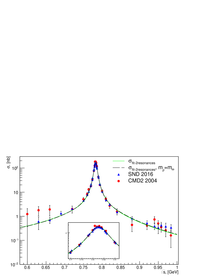
Figure 4: Fits of the $\rho-\omega$ peak with 2 resonances. Insert is zoom in of the peak.

Table 1: Values of $\chi^{2}$ for fit with 2 resonances.

	CMD2	SND2016	CMD2+SND2016
$\chi^{2}/d.o.f.$	2.29	1.46	1.71

From other side, such small value as the difference between $\rho$ and $\omega$ mesons masses is clearly out of the the accuracy of the ASR approach. That’s why we perform one more fit using (16), supposing that $m_{\rho}=m_{\omega}$ and $s_{3\rho}=s_{3\omega}=m_{\rho}^{2}=m_{\omega}^{2}\approx 0.61\ GeV^{2}$, but with PDG [20] values for widths: $\Gamma_{\rho}=0.149\ GeV,\Gamma_{\omega}=0.00849\ GeV.$ The result is shown on the Fig.4(dashed line), the values of the fit parameters are the same: $\alpha=0.52,\ \beta=0.49;$ and the values of $\chi^{2}$ are in the Table2.

Table 2: Values of $\chi^{2}$ for fit with 2 resonances with $m_{\rho}=m_{\omega}$.

	CMD2	SND2016	CMD2+SND2016
$\chi^{2}/d.o.f.$	2.12	1.07	1.42

As one can see from the Fig.4 and Tables 1, 2, the both variants have very good agreement with data. Note, that the second one describes data even better than the first one.

In the limit of real photon $q^{2}\rightarrow 0$ and neglecting $\Gamma_{\rho},\Gamma_{\omega}$ the pion TFF takes form:

$$F(0)=\frac{1}{2\sqrt{2}\pi^{2}f_{\pi}}(\alpha+\beta).$$

And correspondingly one can find

$$\Gamma(\pi^{0}\rightarrow 2\gamma)\approx 7.9\ eV,$$

which is in the perfect agreement with experimental data [21].

3.3 $\phi$ peak

Let us now consider the second peak. Theoretical estimations shows( work is now in progress), that the such kind of a peak can appear, if one takes into account $\pi-\eta-\eta^{\prime}$ mixing and s-quark masses into the anomaly sum rules. Thus, in this case the pion TFF will have 3 terms. So, in addition to the terms corresponding to $\rho$ and $\omega$ mesons, one should add a term corresponding to the $\phi$ meson ( the value of $m_{\phi}=1.0194\ GeV$ and the value of $\Gamma_{\phi}=0.00426\ GeV$ were taken from PDG [22]. ). Let us suppose, that $s_{3\phi}$ will be close to the $m_{\phi}^{2}$ and $m_{\rho}=m_{\omega},s_{3\rho}=s_{3\omega}=m_{\rho}^{2}=m_{\omega}^{2}=s_{3}\approx 0.61\ GeV^{2}.$ Thus, we got:

$$F(q^{2})=\frac{1}{2\sqrt{2}\pi^{2}f_{\pi^{0}}}\left(\alpha\frac{s_{3}}{s_{3}-q^{2}+im_{\rho}\Gamma_{\rho}}+\beta\frac{s_{3}}{s_{3}-q^{2}+im_{\omega}\Gamma_{\omega}}+\gamma\frac{s_{3\phi}}{s_{3\phi}-q^{2}+im_{\phi}\Gamma_{\phi}}\right).$$ (18)

Substituting the eq.(18) to (11), one obtains the equation for the total cross section. The result of the fit is shown on the Fig.5, values of the fit coefficients are: $\alpha=0.556,\ \beta=0.49,\ \gamma=-0.036$. The $\chi^{2}$ values are in the Table3.

Table 3: Values of $\chi^{2}$ for fit with 3 resonances.

	CMD2	SND2016	CMD2+SND2016
$\chi^{2}/d.o.f.$	2.53	1.52	1.87

As one can see from the Fig.5, the fit with 3 resonances gives good description of experimental data. In the same way, as was discussed in the end of the previous section, by use of (18) we can obtain in the limit $q^{2}\rightarrow 0$ the value

$$\Gamma(\pi^{0}\rightarrow 2\gamma)\approx 7.9\ eV$$

in good agreement with experiment [21]. We found that the coefficient $\gamma$ is negative, which is dictated by the interference term in the vicinity of $\phi$ peak. Moreover, allowing for the phase shift between $\phi$ and $\rho,\omega$ to be close to $\pi$, supporting negative $\gamma$.

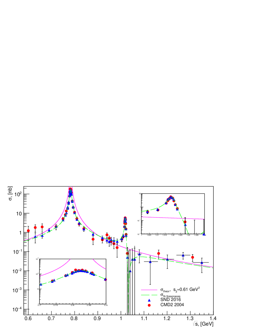
Figure 5: Fit of the whole data range. The inserts are zoom in $\rho-\omega$ and $\phi$ peaks.

Let us pay attention to the coefficient $\gamma$, it is found to be small. As it was mentioned before in the text, the third term in (18) can appear due to effects of $\pi-\eta-\eta^{\prime}$ mixing. So the coefficient $\gamma$ corresponds to the mixing angle $\theta_{\pi-\eta}$. Theoretical prediction of the mixing angle value $\theta_{\pi-\eta}$ was done in the works [23], [24] (and also see [25]:

$$\theta_{\pi-\eta}=\frac{1}{\sqrt{3}}\frac{m_{u}-m_{d}}{m_{u}+m_{d}}\cdot\frac{m^{2}_{\pi}}{m^{2}_{\eta}}=-0.0150\pm 0.020.$$ (19)

Note, that the values of the coefficient $\gamma$ and the mixing angle $\theta_{\pi-\eta}$ are consistent by the order of magnitude. This consistency provides additional support to our assumption about origin of the third term of (18).

Due to the fact that $\phi$ meson has very narrow width, the contribution of the third term is non-negligible only at the region of the $\phi$ resonance, and thus, it can be safely neglected everywhere, except resonance region. Note, that the fit of total cross section with 3 resonances(dashed line) differs from the total cross section with a single pole (11)(solid line) by $\approx 10\%$ at $\sqrt{s}=1.3\ GeV$. And the difference between them decreases with the increasing of the $q^{2}$, thus, as we mentioned earlier in the text, in region far from the poles the total cross section with resonances coincides with the single pole total cross section.

As the result of the analysis of the fits, one can conclude that the modified equation for the pion TFF (18) and the corresponding total cross section shows rather good agreement with the experimental data. The whole spectrum of the data probably can be described if one takes into account the mixing in axial channel. Thus, in the modified ASR approach, which will be taking into account the effects of the $\pi-\eta-\eta^{\prime}$ mixing and small corrections (as well pertubative as non-pertubative), the equation of the pion TFF will contain three terms. Theoretical estimations show that the coefficients $\alpha,\beta$ and $\gamma$ of the eq.(18) can be expressed in terms of the mixing angles $\theta_{\eta-\eta^{\prime}}$, $\theta_{\pi-\eta}$, $\theta_{\pi-\eta^{\prime}}$. The results of the fits provide hard restrictions to the expected values of $\pi-\eta-\eta^{\prime}$ mixing angles and parameters of the modified ASR approach. The work now is in progress.

4 Conclusions and Outlook

1. We show that the result obtained in the paper [15] for the pion timelike TFF (8), can be used to describe the data in the regions far from the pole, and the place of the pole coincides with the experimental peak. It has been shown, that eq.(8), and the corresponding equation of the total cross section eq.(12), has better agreement with the data if $s_{3}\approx 0.61GeV^{2}$. This one coincides with the result of matching ASR and LCSR [19] that $s_{3}$ should vary between $0.67\ GeV^{2}$ at large $q^{2}$ and $0.61\ GeV^{2}$ at low $q^{2}$.

2. We propose a modification of the equation of the pion TFF in order to describe the data at the resonance regions. As a result of the analysis, we may conclude that in order to describe the whole spectrum of data, one should obtain formula of the pion TFF containing three terms. Using modified equation of the pion TFF 18, we perform fits of the experimental data and obtain the values of the fit coefficients. The obtained result provides a good description of the experimental data, including the correct limit for the case of real photons($q^{2}\rightarrow 0$).

3. To obtain three terms in the pion TFF within the ASR approach one should include the effects of the $\pi-\eta-\eta^{\prime}$ mixing. Let us stress, that the obtained value of the fit coefficient $\gamma$ corresponding to the third term (18) has the same order of the magnitude as the $\theta_{\pi-\eta}$ mixing angle. So it confirms our assumptions. The achieved values of the fits coefficients lead to strong restrictions to the values of the $\pi-\eta-\eta^{\prime}$ mixing angles and can be used in matching with the theoretical values, calculated, in particular, in the modified ASR approach.

The work was supported in part by RFBR grant 14-01-00647.

References

- [1] H. J. Behrend et al. [CELLO Collaboration], Z. Phys. C 49, 401 (1991).
- [2] J. Gronberg et al. [CLEO Collaboration], Phys. Rev. D 57, 33 (1998).
- [3] B. Aubert et al. [BaBar Collaboration], Phys. Rev. D 80, 052002 (2009) [arXiv:0905.4778].
- [4] S. Uehara et al. [Belle Collaboration], Phys. Rev. D 86, 092007 (2012) [arXiv:1205.3249].
- [5] G.P. Lepage and S.J. Brodsky, Phys. Rev. D 22, 2157 (1980).
- [6] D. M. Asner, T. Barnes, J. M. Bian, I. I. Bigi, N. Brambilla, I. R. Boyko, V. Bytev and K. T. Chao et al., Int. J. Mod. Phys. A 24, S1 (2009) [arXiv:0809.1869].
- [7] D. Babusci, H. Czyz, F. Gonnella, S. Ivashyn, M. Mascolo, R. Messi, D. Moricciani and A. Nyffeler et al., Eur. Phys. J. C 72, 1917 (2012)[arXiv:1109.2461].
- [8] M. N. Achasov et al. , Study of the reaction with the SND detector at the VEPP-2M collider, Phys. Rev. D 93, 092001 (2016), [arXiv:1601.08061 [hep-ex]].
- [9] CMD2 Collaboration:Study of the Processes , in the c.m. Energy Range 600-1380 MeV at CMD-2, Phys.Lett. B605 (2005) 26-36, [arXiv:hep-ex/0409030v2] .
- [10] M. Hoferichter, B. Kubis, S. Leupold, F. Niecknig, S. P. Schneider, Dispersive analysis of the pion transition form factor, [arXiv:1410.4691 [hep-ph]]
- [11] M. J. Amaryan, M. Bashkanov, M. Benayoun, F. Bergmann, J. Bijnens, L. C. Balkest, H. Clement and G. Colangelo et al., MesonNet 2013 International Workshop. Mini-proceedings, [arXiv:1308.2575].
- [12] J. Horejsi, O. Teryaev, Dispersive approach to the axial anomaly, the t’Hooft principle and QCD sum rules, Z. Phys. C65, 691-696 (1995).
- [13] Y. N. Klopot, A. G. Oganesian and O. V. Teryaev, Axial anomaly as a collective effect of meson spectrum Phys. Lett. B 695, 130 (2011)[arXiv:1009.1120].
- [14] B.L.Ioffe, Axial anomaly: the modern status, Int.J.Mod.Phys.A21:6249-6266,2006, [arXiv:hep-ph/0611026]
- [15] Y.Klopot, O.V. Teryaev, A. Oganesian, Axial anomaly and vector meson dominance model, JETP Lett. 99 (2014) 679-684, [arXiv:1312.1226 [hep-ph]].
- [16] G. ’t Hooft et al.,Recent developments in gauge theories, Plenum Press, New York, 1980
- [17] A. V. Radyushkin,Quark-Hadron Duality and Intrinsic Transverse Momentum, Acta Phys. Polon. B 26, 2067 (1995) [hep-ph/9511272].
- [18] M. A. Shifman, A. I. Vainshtein and V. I. Zakharov, Nucl. Phys. B 147, 448 (1979).
- [19] A.G.Oganesian,A.V.Pimikov,N.G.Stefanis,O.V.Teryaev, Matching lightcone- and anomaly-sum-rule predictions for the pion-photon transition form factor, Phys.Rev. D 93, 054040 (2016),[arXiv:1512.02556 [hep-ph]]
- [20] K.A. Olive et al. (Particle Data Group), Chin. Phys. C, 38, 090001 (2014) and 2015 update,
- [21] Kees de Jager, Recent Experimental Results from JLab, Prog.Part.Nucl.Phys.61:311-324,2008, [arXiv:0801.4520v1 [nucl-ex]]
- [22] K.A. Olive et al. (Particle Data Group), Chin. Phys. C, 38, 090001 (2014) and 2015 update,
- [23] B.L.Ioffe, Yad.Fiz. 29 (1979) 1611.
- [24] D.G.Gross, S.B.Treiman and F.Wilczek, Phys.Rev. D19 (1979) 2188.
- [25] B.L. Ioffe, A.G. Oganesian, Axial anomaly and the precise value of the gamma decay width, Phys.Lett. B647 (2007) 389-393, [arXiv:hep-ph/0701077v2].