Perfecting the Photometric Calibration of the ACS CCD Cameras

Abstract

Newly acquired data and improved data reduction algorithms mandate a fresh look at the absolute flux calibration of the CCD cameras on the Hubble Space Telescope (HST) Advanced Camera for Surveys (ACS). The goals are to achieve a 1% accuracy and to make this calibration more accessible to the HST guest investigator. Absolute fluxes from the CALSPEC database for three primary hot 30,000–60,000K WDs define the sensitivity calibrations for the WFC and HRC filters. The external uncertainty for the absolute flux is $\sim$1%, while the internal consistency of the sensitivities in the broadband ACS filters is $\sim$0.3% among the three primary WD flux standards. For stars as cool as K type, the agreement with the CALSPEC standards is within 1% at the WFC1-1K subarray position, which achieves the 1% precision goal for the first time. After making a small adjustment to the filter bandpass for F814W, the 1% precision goal is achieved over the full F814W WFC field of view for stars of K type and hotter. New encircled energies and absolute sensitivities replace the seminal results of Sirianni et al. that were published in 2005. After implementing the throughput updates, synthetic predictions of the WFC and HRC count rates for the average of the three primary WD standard stars agree with the observations to 0.1%.

1 Introduction

Photometric calibration uncertainties are the dominant source of error in current type Ia supernova dark energy studies and other cosmology efforts; and the precision of the constraints on the constants in the Einstein equations of general relativity are directly related to the precision of absolute flux calibrations (Scolnic et al., 2014).

The ACS CCD (charge coupled device) flux calibration was updated fairly recently in a series of four Instrument Science Reports that covered the philosophy and techniques, including charge transfer efficiency (CTE) corrections, encircled energy (EE) corrections, changes in sensitivity with time, and the absolute flux calibration itself (Bohlin & Anderson, 2011; Bohlin, 2011; Bohlin et al., 2011; Bohlin, 2012). However, additional data, updates to the processing, and revised fluxes for the primary standard stars, which change by up to $\sim$1% (Bohlin & Proffitt, 2015), mandate a fresh analysis of the complete body of calibration observations. ACS has two CCD channels and a Solar Blind Channel (SBC). The CCD channels are a Wide Field Channel (WFC) and a High Resolution Channel (HRC), both of which ceased functioning in 2007. However, the WFC was revived during Servicing Mission four (SM4) in 2009.

Changes to the data reduction with generally sub-percent effects include: updated bias reference files, a better removal of the weak striping in data obtained with the new electronics installed during SM4, a refined correction for the sensitivity degradation with time, and a fix of a minor flaw in the calculation of the sky background in the IDL $apphot.pro$ routine used to extract the photometry of the standard stars from the _crj.fits files. The low level striping in the post-SM4 WFC data is removed using the median for each row, which works nicely for the sparse standard star fields in the 1024x1024 subarrays after masking a 5.5x5.5″ box centered on the star. The Space Telecope Science Institute (STScI) pipeline data processing begins with the _raw.fits data files, and then applies the flat field correction along with other corrections associated with CCDs to make _flt.fits files. If there are multiple exposures at the same pointing that are taken to permit the rejection of cosmic ray hits, then the _crj.fits files are also produced from the _flt.fits files. If multiple exposures are taken of the same target but with small dithered pointing offsets, then the _flt.fits data are combined with the drizzle software task to make _drz.fits files that have both hot pixels and cosmic ray rejection. The flat fields are designed to produce the same response in each pixel when observing a perfectly uniform diffuse source. However, optical distortions cause variations in the size of the pixels in arcsec on the sky; so that a multiplication by a pixel-area map (PAM) file is required for the _flt.fits and _crj.fits files to correct for the pixel size variation and make a uniform response anywhere in the field for the same stellar point source. The PAM correction is built into the drizzle software; and no PAM correction is needed for the _drz.fits files.

The logical flow of the derivation of the ACS flux calibration starts with extracting the latest version of the standard pipeline data products from the Mikulski Archive for Space Telescopes (MAST). Then, the aperture photometry is extracted from the _crj.fits files for various aperture radii. These photometry data files form the basis for subsequent analyses, including derivation of the fractional encircled energy (EE) as a function of radius, of the change in sensitivity as a function of time on orbit, and of the absolute flux calibration. The main goal of this work is to establish this flux calibration with better than a 1% precision at the WFC1-1K reference point for the heavily used broadband filters. The HST method of parameterizing the instrumental calibration of flux sensitivities relies on pre-launch estimates for the fractional thoughput or quantum efficiency of each element in the optical path from the primary mirror through to the detector that registers the photon events. Instrumental sensitivities depend directly on the product of all these component efficiencies and the collecting area of the 2.4 m primary mirror. In-flight updates to the pre-launch estimates are derived from observations of standard stars with known flux distributions and are implemented via changes to the detector QE as a smooth function of wavelength or by scaler correction factors to the filter throughput functions. In this work, wavelength dependent corrections for two filter bandpass functions are also derived. No new updates to the QE vs. wavelength are needed, so that the calibration reference files that must be delivered for the pipeline data reduction includes only files to define the changing sensitivity vs. time and files that update the filter throughputs.

Section 2 reviews the observational data and its pipeline reduction, while Section 3 covers the details of the bias subtraction. Section 4 augments the EE fractions, which now include apertures of radii from 0.05–2″, i.e. 1–40 WFC pixels. Section 5 reviews the sensitivity change with time; Section 6 justifies a change in the F814W bandpass throughput function; and Section 7 covers the absolute flux calibration for photometry. An analysis of the problematic _drz.fits files appears in the Appendix and shows that more than a quarter of the 334 _drz images of standard stars are erroneous.

The original comprehensive ACS calibration paper (Sirianni et al., 2005) also covered these topics, except for changes in sensitivity with time and wavelength dependent bandpass adjustments. While the (Sirianni et al., 2005) EE results are for the center of the 1024x1024 pixel HRC channel, those WFC EE values are averages of data at the centers of the ACS CCD 1 and CCD 2, which are butted to make the 4096x4096 pixel WFC detector. Any location can be used for the absolute flux calibration,as long as the flat field is perfect in making all locations equivalent. For efficient use of the ACS calibration time, the center of the WFC1-1K subarray is the chosen flux calibration reference point for the WFC. The flat fields are derived from dithered observations of 47 Tuc (Mack et al., 2002); and the pioneering pilot check of these flats with dithered observations of bright standard stars with a wide range of stellar color temperature is Bohlin & Grogin (2015) for F814W and F435W. With the bandpass adjustment of Section 6, F814W is now uniform to 1% for stars of type K and hotter. For F435W, further analysis of these new flat field checks will be forthcoming.

2 Observations

Table 1: Stellar Flux Standards

			Number of Visits
Star	Sp.Type	V	WFC	HRC	STIS
G191B2B	DA.8	11.781	8	2-3	12-17
GD153	DA1.2	13.346	8	2	14-32
GD71	DA1	13.032	7-8	2	17-34
GRW+70∘5824	DA3	12.77	0	4	1-85
BD+17∘4708	sdF8	9.47	2	1-6	3-6
P330E	G2V	13.03	3	1	1-5
KF06T2	K1.5III	13.8	3	0	3
VB8	M7V	16.70	4	3	3
2M0036+18	L3.5	21.34	1	2	2
2M0559-14	T4.5	I=19.14	2	1	1

Table 1 lists the HST standard stars utilized for the flux calibration; and the three primary hot WD stars G191B2B, GD153, and GD71 define the ACS flux calibration and its change over time. Multiple observations of these stars have a sub-percent repeatability and provide a robust measure of the cross-calibration between the Space Telescope Imaging Spectrograph (STIS) and the ACS average response in each filter. For the secondary standards, three separate ACS visits and three STIS measures of their spectral energy distributions (SEDs) are required for each star to provide minimal confirmation of repeatability and $<<$1% statistical significance. Results based on stars with fewer observations are less reliable. The measured STIS SEDs are from CALSPEC (Bohlin, 2014), while ACS data obtained after 2011 July are not previously analyzed. The standards are all observed at the center of the ACS WFC1-1K subarray in order to provide a standard reference point and anchor for the flat field calibrations.

Since the previous analysis by (Bohlin, 2012), the USEAFTER dates for some superbias reference files were adjusted to be earlier. CCD detectors are operated with a positive electronic bias level, so that noise or drifts in the analog circuitry before digitization does not drive the measured charge to negative levels. The pattern in the bias frames taken with zero exposure time changes slowly and must be monitored as a function of time. A USEAFTER date is the time when a reference file first becomes relevant. For example, the bias observations that occurred 4 days AFTER the G191B2B observation on 2011Nov10 now have a USEAFTER of 2011Oct27, so that the bias correction is closer in time than the previously used reference file with a USEAFTER of 2011Aug 25. While the change in the 1″ photometry is negligible ($<$0.02%), the bias is important for the infinite (5.5″) aperture, which changes by up to 0.6%. The EE in the infinite aperture defines the diffuse source calibration, but the point source flux calibration in the smaller apertures is unaffected, as long as the same EE factor for conversion from the smaller standard radius to infinite is used to convert back to the smaller radius. Perhaps, the absolute calibration PHOTFLAM header keyword for infinite aperture should be augmented to include the small aperture EE keyword values for convenience and to avoid erroroneous usage of obsolete EE values.

3 Data Processing

Standard practice for ACS pipeline data processing is to obtain and subtract a CCD bias image, which consists of data obtained within the same CCD anneal cycle (currently every four weeks). Data fetched from the Mikulski Archive for Space Telescopes (MAST) shortly after a program execution should always be re-extracted from the archive after the final bias and dark reference files are delivered with their usual 1–2 month delay. Before the ACS electronics repair in 2009 April on SM4 that included an Application-Specific Integrated Circuit (ASIC) to read the CCD data, the subarray bias could be extracted from the full frame biases; but different clocking speeds in the ASIC for subarrays now mandates separate subarray bias observations. Full frame WFC bias reference files have a regular two-week cadence; but the post-SM4 subarray bias observations occur only as needed in association with the science observations. Originally, a regular cadence of post-SM4 WFC1-1K subarray bias observations executed through 2012 Oct, but calibration programs must now schedule any required bias frames along with the external observation. There are no WFC1-1K bias observations with USEAFTER dates between 2012 Oct 14 and 2014 Sep 3. Of the cooler stars used in this work, the only observations that lie in this WFC1-1K bias desert are for BD+17^∘4708 on 2013 Sep 4 and VB8 on 2013 Mar 11.

Before the proper associated bias data were reduced to reference files, some of the WFC1-1K subarray observations were processed with a bias reference file that was obtained up to 666 days earlier. Aperture photometry of 1″ and smaller is the same to 0.1% for current and out-of-date bias reference files. Even though individual measures with the 5.5″ radius have errors of up to 1%, the effect on the average EE tabulated in the Apendix is less than 0.2% for any filter.

For the flat field mapping program 13602 (Bohlin & Grogin, 2015), the 400x400 subarrays have associated bias observations without overscan columns. Unfortunately, the pipeline data processing requires bias observations with overscan, and the archival 13602 data are processed with the bias data extracted from a full frame bias image. The errors in the 20 pixel radius photometry for the archival MAST versions range up to 1.7% in comparison to the custom reduction of Bohlin & Grogin (2015).

In order to verify consistency with the various community photometry packages, Table 2 includes the extracted $electrons~{}s^{-1}$ used in the current flux calibration for aperture radii of 3, 5, 10, 20, and 110 pixels for the WFC1-1K subarray observations of GD71 obtained at 2003.84 on 2003 Nov 3. The images are j8v602*_crj.fits files, as processed by the CALACS pipeline on 2015 Nov 17 and then corrected by the pixel area map (PAM). Changes from the same 20 pixel 1″ photometry shown in table 3 of Bohlin (2012) are $<0.06\%$. Changes in the sky backgound are similarly neglibible but do become more consistent with a range of -0.024 to 0.094 vs. the previous -0.011 to 0.221 $electrons~{}s^{-1}$.

Table 2: Sample WFC photometry in $electrons~{}s^{-1}$ for GD71 from j8v602*crj.fits files, as corrected by the PAM reference file.

Filter	x (px)	y (px)	exp (s)	3 px	5 px	10 px	20 px	110 px	sky
F435W	497.8	514.5	4.0	127926	140928	147862	153310	163968	-0.007
F475W	497.7	514.9	3.0	162872	180284	189444	196187	210275	-0.024
F502N	497.3	514.9	90.0	4660	5164	5433	5622	5987	0.000
F555W	497.6	514.6	4.6	97517	108059	114029	117966	125763	0.013
F550M	497.6	515.2	10.0	41260	45694	48391	50188	53620	0.001
F606W	497.4	514.6	2.6	171574	190340	201716	208721	220635	0.094
F625W	497.4	514.9	5.0	86432	95947	102064	105772	112404	0.017
F658N	497.9	515.2	120.0	3832	4263	4555	4737	5013	0.001
F660N	498.0	514.5	300.0	1510	1666	1780	1877	1984	0.000
F775W	497.4	514.7	9.0	47405	53338	57179	59280	63064	0.011
F814W	497.9	514.5	8.0	56248	64280	69303	71881	75904	0.004
F892N	1009.2	1025.0	220.0	1638	1955	2139	2221	2383	0.001
F850LP	497.6	515.1	24.0	14872	18050	20056	21079	22641	0.001

4 Encircled-Energy Aperture-Correction Update

4.1 Equations

Following the methodology of Bohlin (2012) but with the improved notation of Bohlin et al. (2014), the photon weighted mean flux over the bandpass in wavelength ($\lambda$) units is

$$\langle F\rangle={\int F_{\lambda}~{}\lambda~{}R~{}d\lambda\over\int\lambda~{}R~{}d\lambda}={S~{}N_{e}}~{},$$ (1)

where our flux $F$ is $erg~{}cm^{-2}~{}s^{-1}~{}\AA^{-1}$, $R$ is the system fractional throughput, i.e., the total system quantum efficiency (QE) as a function of wavelength, S is the instrumental calibration constant photflam that appears in the ACS data headers, $N_{e}$ is the measured instrumental count rate in photoelectrons $s^{-1}$ in the ACS ’infinite’ 5.5″ radius aperture, and the integral is over the bandpass range of the filter. Equation 1 includes all the photons from starlight incident on the primary, regardless of where the light hits the detector, so that $N_{e}$ implicitly includes all the detected photons in an infinite-radius aperture. Of course, an actual infinite radius is not feasible and 5.5″ is about as large an aperture that is practical. In principle, models of the instrumental point spread function (PSF) could help define the encircled energy for an infinite aperture. In the case of HST, considerable effort has been expended on the Tiny Tim PSF modeling software. However, the Tiny Tim user manual states: “Generally, the models are not very good past a radius of $\sim$2″, due to the effects of scatter and high-frequency aberrations” (Krist & Hook, 2004). Because of the small gains in enclosed signal as the aperture size increases toward 5.5″, the error in the infinite aperture estimate should be $<$1%; and this uncertainty applies only to the diffuse source calibration. The precision of the point source flux calibration is not affected by errors in the adopted infinite aperture EE estimate. The sky background annuli are 6-8″ for WFC and 5.6-6.5″ for HRC. The count rate $N_{e}$ can also be predicted from the known instrumental throughput parameters and the known CALSPEC flux $F_{\lambda}$ for each standard star

$$N_{e}={A\over hc}{\int F_{\lambda}~{}\lambda~{}R~{}d\lambda}~{},$$ (2)

so that

$$S={hc\over A\int{\lambda~{}R~{}d\lambda}}~{},$$ (3)

where h is Planck’s constant, c is the speed of light, and A is the collecting area of the primary mirror, taken to be 45,239 $cm^{2}$. The traditional method of flux calibration for HST that is followed in this paper involves adjusting $R$ in Equation 2, so that the computed $N_{e}$ equals the measured count rate. Systematic deviations between the computed and measured $N_{e}$ for all the filters are accounted by smooth adjustments of the detector QE vs. wavelength, while residuals for each filter are corrected by adjusting the filter throughput. The point source calibration $S$ for the infinite aperture is required for computing the diffuse source surface brightness calibration (Bohlin et al., 2014).

For aperture photometry with a radius of $i$, the EE fractions $E_{i}$ are the average of the measured $E_{i}=N_{i}/N_{e}$ for each filter, i.e. the sum of the counts $s^{-1}$ $N_{i}$ within a radius $i$ divided by $N_{e}$; and once the average $E_{i}$ are established, the infinite aperture $N_{e}$ can be computed from any small aperture photometry by dividing by the encircled energy fractions $E_{i}$ that are the aperture corrections used to correct small radius aperture photometry to a larger reference aperture, i.e. the infinite aperture for ACS.

For example, the commonly used 3, 5, 10, and 20 pixel radii for WFC (double for HRC) are approximately 0.15, 0.25, 0.5, and 1 arcsec, where

$$N_{e}=N_{3}/E_{3}=N_{5}/E_{5}=N_{10}/E_{10}=N_{20}/E_{20}~{}.$$ (4)

Thus, the mean flux $\langle F\rangle$ is S N${}_{i}/E_{i}$, where the most appropriate radius subscript can be chosen.

For many science images, the use of the proper sky annulus at 6–8″ is not appropriate and a correction is required to the photometric calibrations presented here that are all based on that fixed sky annulus. Ignoring these corrections for sky annulii of only a few pixels causes photometric errors of a few percent. Because of gradients in the sky background in many science images from the star to the WFC standard sky annulus at 6–8″, smaller sky annuli are often required. However, the stellar signal from the PSF wings that are included in the sky measures must be added to the measured count rate $N_{i}$. The fraction $f$ of the signal in the sky annulus depends on the photometry radius $r_{i}$ and the inner $r_{a}$ and outer $r_{b}$ sky radii. The measured count rate $N_{i}$ must be divided by $(1-f)$ to get the true photometry $N_{i})$, where

$$f={{E_{b}/E_{i}-E_{a}/E_{i}}\over{{r_{b}}^{2}/{r_{i}}^{2}-{r_{a}}^{2}/{r_{i}}^{2}}}~{}.$$ (5)

For example, three pixel WFC photometry $N_{3}$ with $r_{i}=3$, background inner annulus $r_{a}=4$, and outer $r_{b}=6$ has a correction $(1-f)=0.963$ for F850LP according to the EE tables in the Appendix.

4.2 EE Changes over Time

Plots of the aperture photometry vs. time illustrate the reproducability and determine the best aperture for the absolute flux calibration. For example, Figure 1 compares the measured WFC F606W count rate $N_{i}$ to the predicted $N_{e}$ for an infinite aperture for five of the most relevant photometry apertures from three to 110 pixels. The measured photometry for each star is divided by the predicted value in order to preserve the intrinsic rms scatter of the data and avoid large fluctuations that would be caused by dividing by the measured infinite aperture values. The rms scatter is tabulated for all eight of the WFC broadband filters in Table 3. There are no obvious trends with time or with stellar color in Figure 1.

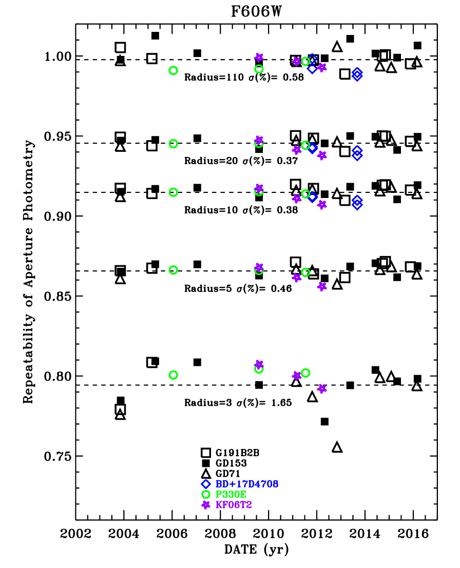
Figure 1: Ratio of the measured WFC count rates Ni to the predicted count rate in an infinite aperture for G191B2B, GD153, GD71, BD+17^∘4708, P330E, and KF06T2. The gap in time from 2007-2009 is when ACS/WFC was not operational. The low point for the three pixel radius GD71 at 2012.8 is not caused by any saturated pixel falling outside the three pixel radius, which suggests that the occasional image has a 3$\sigma$ error (5% here) for three pixel photometry.

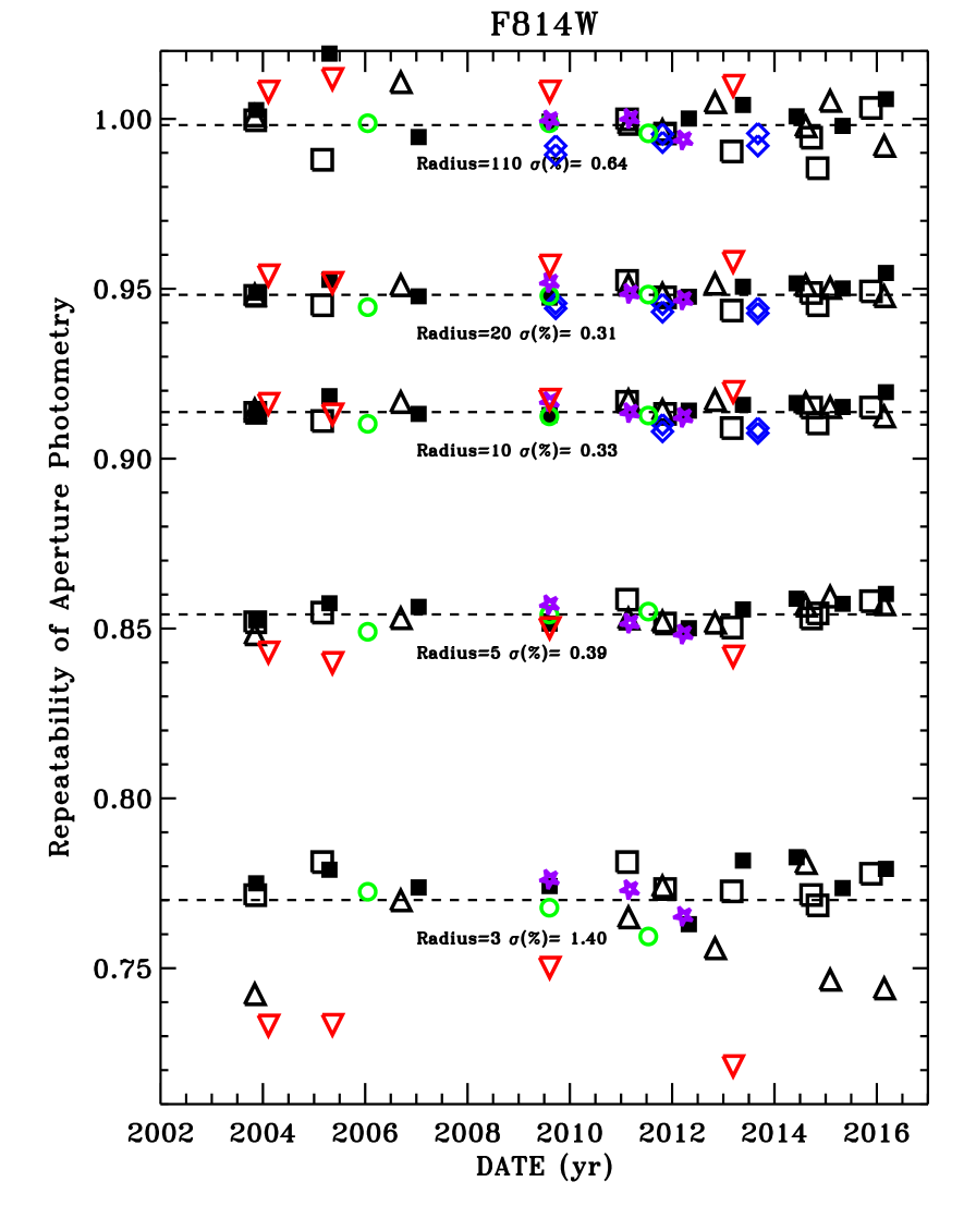
Figure 2: As in Figure 1 for F814W and with the addition of VB8 (red inverted triangles).

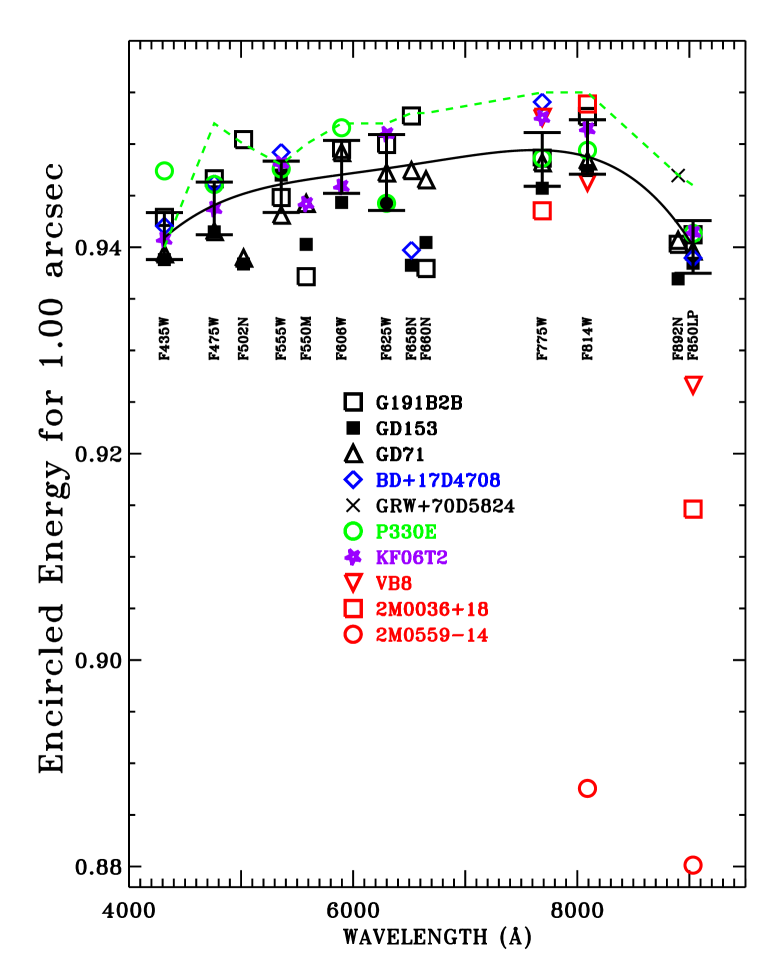
Figure 3: Encircled energy $E_{20}$ for WFC, i.e. fraction of signal in a 1″ aperture relative to an “infinite” aperture of 5.5 arcsec radius. The solid black line is a quartic fit to only the broadband filter EE averages for the WDs, the F star (BD+17^∘4708), the G star (P330E), and the K star (KF06T2). Error bars for the eight filters used for the polynomial fit are $\pm 3\sigma$ errors-in-the-mean of these averages, but the average values are not shown to avoid crowding. The green dashed lines are the corresponding results of Sirianni et al. (2005).

Table 3: Photometric rms Scatter for Various Radii at the WFC1-1K Reference Point

Filter	$\sigma_{3}$(%)	$\sigma_{5}$(%)	$\sigma_{10}$(%)	$\sigma_{20}$(%)	$\sigma_{110}$(%)
F435W	1.00	0.43	0.37	0.35	1.08
F475W	1.76	0.39	0.31	0.30	0.51
F555W	1.26	0.41	0.41	0.41	0.69
F606W	1.65	0.46	0.38	0.37	0.58
F625W	2.00	0.43	0.30	0.30	0.77
F775W	2.23	0.60	0.50	0.51	0.76
F814W	1.40	0.39	0.33	0.31	0.64
F850LP	1.94	0.87	0.58	0.44	0.81

For the bright, isolated standard stars, the 20 pixel ($\sim$1″) aperture generally has the best repeatability at 0.30–0.51% for $\sigma_{20}$ and, therefore, defines the best photometry for each observation, although there is little loss in precision with an aperture as small as five pixels, where 0.39$<\sigma_{5}<$0.87. While the infinite 5.5″ radius aperture contains all the signal by definition, there is more scatter because of the excess sky noise in such a huge aperture. The three pixel radius aperture has up to seven times the uncertainty of a 1″ aperture; and if possible, the use of $E_{3}$ to calibrate science data should be avoided because of exact centering uncertainties and focus variations that could be systematic over an entire image.

Figure 2 is similar to Figure 1, except for the addition of the problematic M star VB8. The infinite (110 pixel) radius values for all four VB8 observations are high by 0.5–1% with respect to the hotter star average. This offset could be caused by a low value of the predicted $N_{e}$ from the STIS SED. In the region of the F814W sensitivity, the VB8 flux is on the short wavelength, rapidily declining side of the SED, where stellar variability is common. In addition, a large contribution to the VB8 predicted count rate is from 9000–9600 Å  where STIS has a low sensitivity and worse rms repeatability. In Figure 2, the 20 pixel radius VB8 points are also high but not as high as the 110 pixel values, which accounts for the slightly low F814W, VB8 average for the WFC in Figure 3. At the three pixel radius in Figure 2, VB8 is significantly low, indicating that there must be some extra loss into the red halo of Section 4.4 for such a small aperture.

4.3 Hot, Early Type Stars

EE values are the measured $N_{i}$ divided by the noisy measured $N_{110}$ values; and fitting techniques are required to lower the uncertainties. While the large 110 pixel infinite aperture should recapture all the trapped and re-emitted charge, the smaller aperture data require a CTE correction. The pipeline processing now supplies the Anderson & Bedin (2010) CTE corrected full frame 4096x4096 pixel images; but CTE corrected subarrays are not provided, so that the WFC1-1K subarrays used here must be corrected for CTE losses in the post-pipeline processing by the method of Bohlin & Anderson (2011). A fit as a function of wavelength for the broad filters of Table 3 reduces the uncertainty, while at the same time providing fitted values for the problematic narrower filters (Bohlin, 2012). Figures 3 and 4 are examples of polynomial fits to the average EE as a function of the pivot wavelength for the 1″ aperture from the hot stars to the K1.5III KF06T2. The plotted symbols are the averages for each star; but the fit is to the global averages of all of the individual observations for each broadband filter. The final results of similar fitting for 12 aperture sizes appear in Table 8 and Table 9 in the Appendix, where typical uncertainties in the EE fits for WFC and the 0.15, 0.25, 0.5, and 1 ″ radii are 0.4, 0.2, 0.4, and 0.1%, respectively. Correspondingly for HRC, the respective uncertainties are 0.4, 0.3, 0.4, and 0.3%. The _flt.fits files must be used for the sometimes saturated WFC data for the bright BD+17^∘4708, because saturated pixels cannot be combined with the cosmic ray rejection algorithm used to produce the _crj.fits files. These final EE values are fits to the measured ratios of the small to infinite aperture count rates, where a few of the later single exposure _flt.fits BD+17^∘4708 observations in the big 5.5″ aperture deviate from the mean by $>3\sigma$ and are omitted. The ACS CCDs are linear through saturation, as long as all of the saturated signal is included in the aperture (Gilliland, 2004), which means that some of the smaller aperture measures of BD+17^∘4708 must also be omitted. The maximum deviation from Sirianni et al. (2005) for the broadband WFC filters is for the three pixel F435W EE value of 0.792, whereas Sirianni et al. (2005) has 0.775.

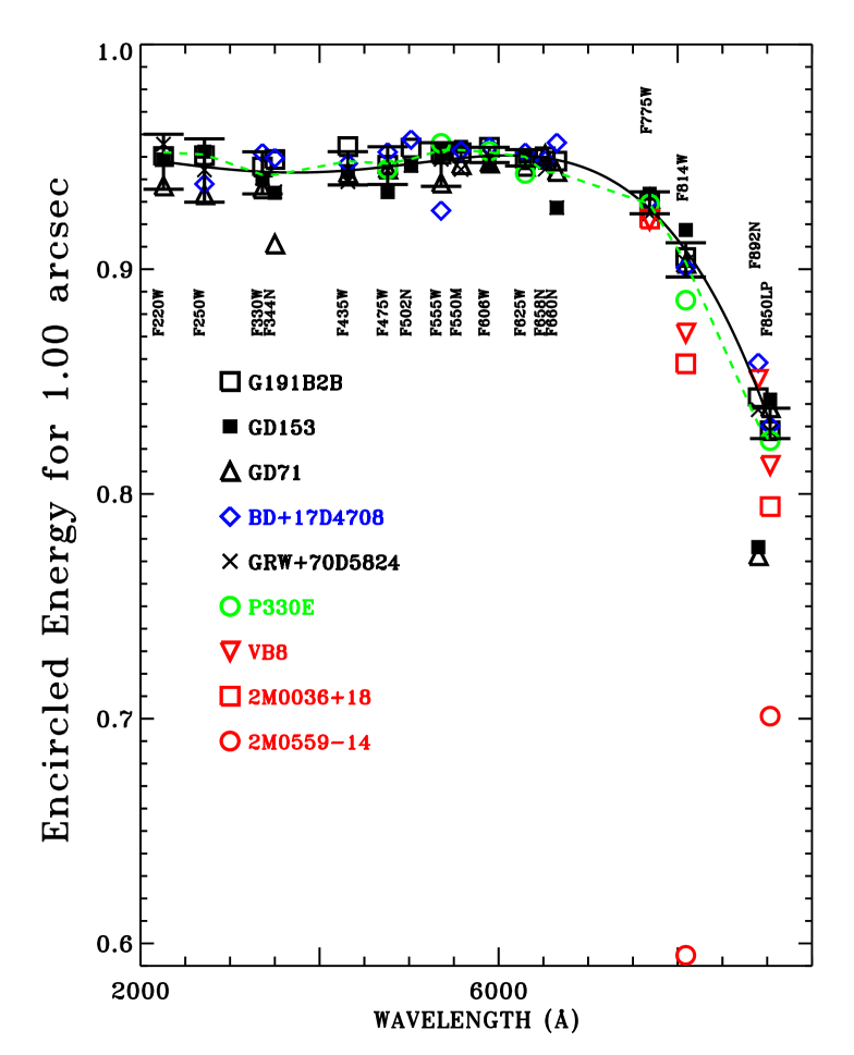
Figure 4: As in Figure 3 for an HRC 1″ aperture, except that there are no data for the K star (KF06T2) and the quartic fit is to the 11 broadband filters that are shown as error bars.

4.4 Cooler, Late Type Stars

For stars redder than KF06T2 (K1.5III), the flux calibration does not achieve the goal of 1% accuracy because of the uncertain EE from the sparsely observed and possibly variable M, L, and T stars. Red stars of spectral type M and later have a “red halo” and show significantly lower EE, because long wavelength photons scatter more in the CCD substrates, especially for HRC, which lacks the special anti-scattering layer incorporated into the WFC CCDs. Figures 3 and 4 show these red star EE values as red data points. Sirianni et al. (2005) provide their tables 6-7, which define the EE vs. effective wavelength. These effective wavelengths are not constant for a filter but increase as the peak of the stellar flux distributions move to longer wavelengths. There is little new data for the three cool stars, so the discussion of uncertainties in Bohlin (2011, 2012) still stands with error bars of $\sim$4% for the Sirianni et al. (2005) EE results for stars of type M and later that are recommended for the WFC filters F814W, F850LP, and F892N and for the HRC filters F775W, F814W, F850LP, and F892N. The only exceptions are for WFC F814W and F892N for the reddest star (T6.5) 2M0559-14, where 0.89 instead of the Sirianni et al. (2005) EE values of 0.94 is recommended for the 20 pixel aperture and 0.84 instead of 0.90 for the 10 pixel aperture. For completeness, some of the most commonly used and recommended Sirianni et al. (2005) EE values for cool stars are in Table 4 for EE values that differ from those in the Appendix for stars of K type and hotter. There are EE values for more radii in Sirianni et al. (2005).

Filter	VB8 (M7)		2M0036(L3.5)		2M0559(T6.5)
	10px    20px		10px    20px		10px    20px
WFC
F814W	…	…	…	…	0.84*	0.89*
F892N	…	…	…	…	0.84*	0.89*
F850LP	0.87	0.93	0.85	0.92	0.78	0.88
HRC
F775W	0.87	0.91	0.86	0.91	0.85	0.90
F814W	0.79	0.86	0.78	0.85	0.75	0.82
F892N	0.77	0.84	0.77	0.84	0.77	0.84
F850LP	0.69	0.78	0.67	0.76	0.55	0.66

Table 4: Encircled energy aperture corrections for very cool stars from Sirianni et al. (2005), except those marked with an asterisk, which are from this work. Use the Appendix EE values for cases not specified here.

4.5 EE Variations around the Field of View

Bohlin & Grogin (2015) investigated the flat field variation for F435W and F814W with two stars at positions spaced around the WFC field-of-view (FOV); and those same data reveal any variation in EE as a function of field position. While the flat fields plus PAM files correct the stellar signal strength to a uniform value around the field in the _crj.fits, there is no correction of the EE for the pixel size or focus variations. Thus, the EE fraction may vary, expecially for small aperture radii. With respect to the Table 8 EE at the WFC1-1K reference point on CCD chip-1, the difference in the EE is measured at the field positions of Bohlin & Grogin (2015) for the 3, 5, 10, and 20 pixel apertures. The expected 1$\sigma$ differences are from Table 3. For example for the average of the two stars, the uncertainty in $E_{20}$, i.e. the 1″ 20 pixel radius divided by the infinite 110 pixel photometry is $\sigma=\sqrt{(0.35^{2}+1.08^{2})/2}=0.8$% for F435W. The only 3$\sigma$ deviations are +2.0–3% larger EE for four of the F814W smaller pixel radii near the (3839,1791) location in the 4096x4096 FOV, eg. 0.873 $\pm 0.005$ instead of the 0.853 $\pm 0.002$ EE in Table 8 for a five pixel radius. However, there are several +2$\sigma$ deviations near the same location in the upper right hand corner of chip-2 for both F435W and F814W. Thus, systematic differences in EE around the field are possible with a range of $\pm$1% for 20 pixels to $\pm$2% for five pixel radius and $\pm$3% for three pixel radius.

In summary, the best chance of achieving the 1% photometry goal is to place the target star at the well characterized WFC1-1K reference point, where several measures of several stars reduce the uncertainties in the average EE to 0.1–0.3%.

5 Changes in Sensitivity with Time

In order to specify a flux calibration for the ACS CCD imaging data, the photometry must be corrected for gradual losses in the instrumental throughput since the installation of ACS into HST on 2002 March 7 (2002.16). The side-1 electronics failure occurred on 2006 Jan 27 (Bohlin et al., 2011); and the activation of the side-2 electronics with the reduction of the set-point temperature from -77C to -81C for the WFC CCD on 2006 July 6 (2006.50) introduced a discontinuity in sensitivity (Mack et al., 2007). In addition, the lowering of the set-point to -81C caused minor flat field changes of up to 0.6%, which are automatically included in the STScI ACS pipeline data products (Gilliland et al., 2006). A second discontinuity in sensitivity is due to the CCD Electronics Box Replacement (CEB-R) with its ASIC sidecar circuit board during the HST Servicing Mission SM4 in 2009 May at 2009.4 (Grogin et al., 2010).

This work updates the results of Bohlin et al. (2011), where more details about the analysis are provided. The reference positions for the flux calibration are at the center of the HRC CCD and at the center of the standard WFC1-1K subarray at pixel (3583,1535) on chip-1; and the change in sensitivity is determined by the photometry with the best repeatability, i.e. the 1″ $N_{20}$ photometry of the three HST primary WD standard stars G191B2B, GD153, and GD71. The sub-percent CTE corrections of Bohlin & Anderson (2011) are applied for WFC and should be negligible for the early HRC data, which is heavily exposed. The three stars are on a common scale defined by their observed infinite-aperture count rate C=$N_{20}/E_{20}$ divided by the predicted total count rate $P=N_{e}$ from the synthetic photometry of Equation 2. The P values depend only on the stellar flux and the system throughput for the filter and are corrected only for the discontinuity due to the change in the WFC temperature from -77C to -81C. The stellar SEDs for these three fundamental HST standards are the measured STIS fluxes on the HST scale (Bohlin, 2014) from the HST CALSPEC database.

For the first years of ACS operations, the change in response that is measured by C/P for each filter is fit with a straight line; and then to reduce measurement noise and enforce the prior of the expected smooth change with wavelength, these line slopes are fit with a polynomial as a function of the filter pivot wavelengths as shown in Figure 5 for the broadband filters available to both WFC and HRC. The HRC and WFC photometry are in red and black, respectively, along with their separate linear fits. The P values for WFC are corrected for the first sensitivity discontinuity for the switch of the set-point temperature from -77C to -81C at 2006.5 (Mack et al., 2007) but are NOT adjusted for the second discontinuity at 2009.4 for the SM4 repair. While the HRC red solid lines are the actual linear least-square fits to the data, the WFC pre-SM4 fits are for the constant term only and adopt the final fitted slopes from Figure 6, in order to get the best estimate of the post-SM4 normalization level. The WFC fits generally appear to agree with the data within the rms noise. However for F850LP, the positive slope of 0.06%/yr from Figure 6 and Table 5 is clearly a better fit to the minimal WFC data.

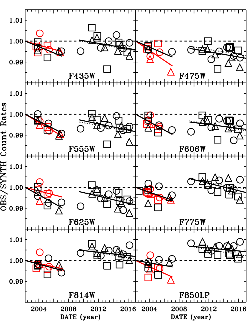
Figure 5: Ratio of observed one arcsec radius photometry to predicted count rates for eight broadband filters as a function of time. The observed count rate is corrected for EE and CTE. Symbols are: square-G191B2B, circle-GD153, and triangle-GD71. Black symbols are for WFC, and red are HRC. The solid line fits and all of the data for each camera are normalized to the value which makes each fit equal to unity at 2002.16. The dotted lines are the parameterized fits used by the routine $acs\_timecorr.pro$, where after 2009.4, the slope is set to the average of -0.061%/yr; and the value at 2009.4 is from Figure 7. For the pre-SM4 WFC, the dotted and solid lines coincide.

For the pre-SM4 ACS epoch, the data are rather sparse, because the policy of the once per year monitoring of the sensitivity changes at the WFC1-1K reference point with the three primary standard stars had not yet been established. The filter F814W is typical of the better data sets with seven WFC data points that agree well with the seven HRC observations, as shown in Figure 5. F475W is a worst case, where there are only four WFC data points; and the main constraint on the rate of sensitivity loss is the lone GD153 point at 2007.0 from program 11054. The planned observations of G191B2B in that cycle 15 were not executed because of the ACS failure at 2007.1. Given the scatter in the data, the WFC loss rate is uncertain but would coincide with the slope from the fitted results, if the lone 2007.0 point that has all the leverage on the fit were $\sim$1$\sigma$ lower. Furthermore, the lone HRC point at 2006.9 for GD71 is probably a low statistical outlier. Statistically, the best result is from accepting both the WFC and HRC measures and adopting the fitted mean for F475W.

Bohlin et al. (2011) present a figure 1 for F555W that is similar to F555W in Figure 5, but where the results for GD153 are systematically low by a fraction of a percent. In particular, the GD153 observation at 2009.6 was below the fit by 0.7%, while the revised results for F555W have this same data point with the typical scatter of only 0.4% low. The primary reason for this improvement among all the analysis updates listed in the Introduction is that the new CALSPEC fluxes for GD153 in the 5500Å region are $\sim$0.4% lower with respect to the other two primary standards, which makes the denominator smaller and raises that point to only $\sim$1$\sigma$ below the fit. Now, the F555W scatter is typical of the other filters, and the Bohlin et al. (2011) anomaly is remedied.

For the later years of ACS after SM4 at 2009.4, the eight WFC broadband filters are well monitored with $\sim$18 visits; and all show a consistent sensitivity loss with a statistical significance ranging from 0.9 to 2.4$\sigma$. This average post-SM4 loss rate is 0.00061 per year, i.e. 0.061%/yr with an error-in-the-mean of 0.007%/yr, which differs at most by $<1\sigma$ from the measured rate of 0.035 $\pm 0.037$%/yr for F850LP. The average loss rate of 0.061%/yr is adopted for all WFC data after 2009.4. The general trends of reduced loss rates with time and increased loss rates toward UV wavelengths are the expected behavior for a gradually slowing outgassing of hydrocarbons and their polymnerization on the optical surfaces. The observed trends in STIS follow this model.

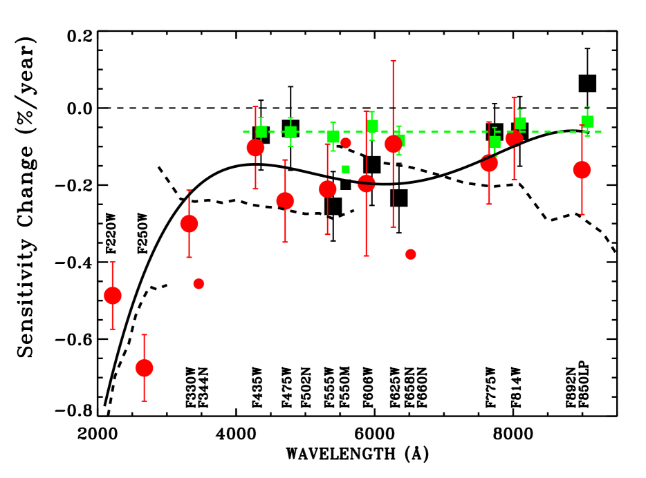
Figure 6: Percent loss of sensitivity ($100{\Delta}S$) per year for all filters, as in Figure 5. Black is for the pre-SM4 WFC, red represents the pre-SM4 HRC, and green is the post-SM4 WFC. Large symbols with error bars are broad bandpass, while small symbols are for the narrow and medium band filters. A fourth order fit (solid black line) to the large pre-SM4 symbols is shown as a function of the filter pivot wavelength, while the green dashed line is the average post-SM4 loss rate. Error bars are the 1$\sigma$ formal uncertainty in the slope of the linear fits. All but three of the error bars cross the fits. The black dashed lines are the average sensitivity losses over the 2002-2007 time frame for the three CCD grating modes of STIS (Stys et al., 2004) and are similar to the ACS loss rates. Because an increase in sensitivity seems non-physical, the pre-SM4 fit for F850LP is forced to the more robust post-SM4 average.

Following Bohlin et al. (2011), Figure 6 shows the slope of the rates of sensitivity loss (${\Delta}S$) for each filter and a fourth-order polynomial fit to the pre-SM4 data for both cameras as a function of the pivot wavelength ($\lambda$).

$${\Delta}S=a+b\lambda+c\lambda^{2}+d\lambda^{3}+e\lambda^{4}$$ (6)

The medium and narrow band data are shown but are omitted in the fitting procedure because of the minimal ACS observation sets and also because of the finite STIS resolution that affects the predicted count rate P. The F850LP WFC and HRC 1$\sigma$ error bars nearly touch, and the other seven broadband pairs of 1$\sigma$ error bars all overlap. There are no systematic differences between the two cameras; and thus, the HRC and WFC slopes are fit together. Among the 16 data points for the eight pairs of WFC and HRC broadbands, only the WFC F850LP lies more than 1$\sigma$ from the fourth-order fit; and the 1$\sigma$ uncertainty of 0.08%/year in the fit encompasses most of the pre-SM4 measurements. The coefficients of the fourth order polynomial, pre-SM4 fit in Figure 6 are a=-0.044561, b=3.0376e-05, c=-7.7328e-09, d=8.3760e-13, e=-3.2569e-17, while the loss rates evaluated at the average pivot wavelengths appear in Table 5 along with the measured values. The fitted loss rates also appear in mag/year for comparison with the pre-SM4 47 Tuc results of (Ubeda & Anderson, 2013) for the WFC. The two entirely different methods agree with a maximum difference in slope of 0.017–0.0018 mag/year for F475W, F658n, and F660N, where (Ubeda & Anderson, 2013) have their largest uncertainties of 0.0015–0.018 mag/year. The main difference in the two methods is that Ubeda & Anderson (2013) did not enforce the prior of a smooth variation of the loss rates vs. wavelength. The STIS loss rates appear as dashed lines in Figure 6 and suggest that the ACS sensitivity losses should also be a smooth function of wavelength. The overall level and not the slopes of the STIS loci should be compared to ACS, because the STIS slope is affected by the grating blaze shifts due to sublimation of the epoxy that bonds the replica gratings to the subtrate.

Filter	Pivot-WL	WFC (%/yr)	HRC (%/yr)	fit (%/yr)	mag/yr	Ubeda	2009.4
F220W	2257	…	-0.49	0.66	0.0072	…	…
F250W	2714	…	-0.68	0.41	0.0045	…	…
F330W	3362	…	-0.30	0.22	0.0024	…	…
F344N	3433	…	…	0.20	0.0022	…	…
F435W	4319	-0.07	-0.10	0.15	0.0016	0.0027	1.000
F475W	4747	-0.05	-0.24	0.16	0.0017	0.0034	0.998
F502N	5023	…	…	0.17	0.0018	0.0012	0.997
F555W	5361	-0.26	-0.21	0.18	0.0020	0.0018	0.996
F550M	5581	-0.20	-0.09	0.19	0.0020	0.0024	0.996
F606W	5921	-0.15	-0.20	0.20	0.0021	0.0011	0.997
F625W	6311	-0.23	-0.09	0.20	0.0021	0.0030	0.998
F658N	6584	…	…	0.19	0.0021	0.0039	0.999
F660N	6599	…	…	0.19	0.0021	0.0039	0.999
F775W	7692	-0.06	-0.14	0.12	0.0014	0.0016	1.004
F814W	8057	-0.06	-0.08	0.10	0.0010	0.0019	1.005
F892N	8915	…	…	0.06	0.0007	…	1.007
F850LP	9033	+0.06	-0.16	0.06	0.0007	0.0014	1.007

Table 5: Sensitivity changes for each CCD filter. The units of the pivot wavelength column are Angstroms. Columns 3–4 are the measured pre-SM4 loss rates in %/yr for WFC and HRC, respectively, while Column 5 is the average pre-SM4 loss rate from the evaluation of the quartic fit to both cameras, as shown in Figure 6. The negative signs are omitted in columns 5–7. The narrow band measurements are generally unreliable and are not tabulated, so that the fitted values must be used. Columns 6 and 7 compare the fitted pre-SM4 loss rates in $mag~{}yr^{-1}$ from the current analysis to the results from the 47 Tuc analysis of Ubeda & Anderson (2013). For the post-SM4 WFC observations, the final column specifies the 2009.4 sensitivities relative to 2002.16 per the curve in Figure 7.

Figure 7: The WFC sensitivity correction at 2009.4 relative to the initial sensitivity at 2002.16 as based on fitting the post-SM4 observations of the three primary WD standard stars. The filled squares are the eight WFC broadband filters, while the smooth curve is a cubic fit to these eight points. The open diamonds are the medium and a narrow band filter.

The sensitivities for each WFC filter after SM4 are based on the fits to $\sim$18 available WD observations for each of the eight broadband filters, as illustrated by the solid lines in the Figure 5. The typical 1$\sigma$ rms scatter of 0.003 about the fits establishes the uncertainty of an individual C/P value. These fits evaluated at 2009.4 appear in Figure 7, where each value represents the sensitivity at 2009.4 relative to the initial sensitivity at 2002.16. However, the QE curve for the -81C set point temperature is used for the post-SM4 calibration, so that the Figure 7 corrections must be applied to the post-2006.5 -81C QE, as this QE is used to calculate the post-2009.4 sensitivities. Because this -81C QE is designed to match the photometry to the -77C 2002.16 QE calibration, this approach also matches the post-2009.4 fluxes to the 2002.16 flux scale. The cubic fit in Figure 7 has coefficients as in Equation 6 of a=1.1536, b=-7.2839e-05, c=1.0806e-08, d=-5.0274e-13, and e=0 as a function of wavelength in Angstroms, while the final column of Table 5 has the evaluations of this cubic at the pivot wavelengths.

Originally, the post-SM4 calibration was set by adjusting the post-SM4 gain to match the 2002.4 epoch photometry of 47 Tuc for F606W (Bohlin et al., 2011). Figure 7 and Table 5 show that an additional small shift in sensitivity by 0.997 improves the match at F606W, while the adjustments range from 0.996–1.007 for the other filters at 2009.4. The post-SM4 corrections at 2009.4 in Table 5 along with the average loss rate of 0.061%/yr determine the post-SM4 $photflam$ flux calibration for the time of the observation as detailed in Section 7.

6 Bandpass Shifts

After fully correcting the photometry for the three primary WD standards, their average C in relation to the synthetic predictions P, i.e. $\langle C/P\rangle$, is unity after making the calibration updates in the following section. Any systematic offset in the C/P for a cooler star is suggestive of errors in the bandpass response function. For example, Bohlin (2012) found that the bandpass function for F435W required a shift of the long wavelength cutoff of +18 Å at the WFC1-1K reference point; and there are lab measures for all the broad filters that show bandpass variations of this order. Figure 8 illustrates the SEDs of the stars used for bandpass adjustments along with the system throughput of the WFC broadband filters. Shifting the effective wavelength of a filter changes the relative response of hot to cool stars. For example, moving F435W (shortest wavelength black line in the lower panel) to longer effective wavelengths decreases the response to hot WDs (black line SED), while increasing the signal for the K star (purple line SED).

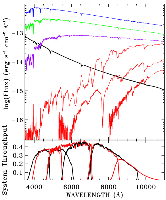
Figure 8: upper panel: SEDs of stars used in this paper with the same color coding as for Figure 3. The solid black line is the WD GD153, and the slopes of G191B2B and GD71 are similar. The red curves in order of bright to faint are VB8, 2M0036+18, and 2M0559-14. For clarity, the SEDs for P330E (green), KF06T2 (purple), 2M0036+18, and 2M0559-14 are scaled up by factors of 12, 8, 4, and 5, respectively. lower panel: The system throughput of the eight WFC broadband filters alternates between black and red lines.

For both F435W and F814W, there are now at least 14 measurements of C/P spaced over the WFC FOV for the K1.5III star KF06T2 with respect to the WD GD153 (Bohlin & Grogin, 2015). Both stars are observed and differences are computed at each of the field positions, so that the hot–cool star offsets are unaffected by any flat fielding errors. The F814W C/P fractional offset of the K star from the WD ranges up to $\sim$-1.5%, while the K star is offset by -0.005 (-0.5%) in C/P at the WFC1-1K reference point based primarily on three observations of KF06T2. Figure 9 illustrates the -16 Å bulk shift of the entire F814W bandpass transmission function, which corrects this offset of -0.005 at WFC1-1K. While the -16 Å correction is precise for KF06T2, the C/P value for the G star agrees within its $3\sigma$ error bar, the variable F star BD+17^∘4708 (Bohlin & Landolt, 2015) is slightly low, and the less reliable M star VB8 moves from 1% low to $\sim$0.5% high. Over the full FOV, the maximum residual offset for KF06T2 with the new -16 Å shift becomes -0.01, i.e. a 1$\pm 0.4\%$ error, which is now within our 1% precision goal for the ACS flux calibration for the first time. With a C/P based primarily on only three F814W observations of the K star at WFC1-1K and without the confirming observations spaced over the full FOV, an adjustment for a sub-percent bandpass discrepancy is not justified. A bulk shift for F814W is better than shifting the usually suspect long wave cutoff, because the photometry is relatively insensitive to the cutoff wavelength; and an unreasonably large shift of $\sim$5 times the bulk shift of -16 Å is required to make the same adjustment of the K star photometry with respect to the WDs. The new bandpass reference files for F435W and F814W are in the ACS calibration database.

Figure 9: F814W C/P and 3$\sigma$ errors-in-the-mean at WFC1-1K for the three primary WD standards and four cooler stars shown as a function of the ratio of the stellar flux across the bandpass from 8920 to 7063 Å. In the lower panel for the original bandpass function, the cooler stars are systematically too faint in comparison to their synthetic photometry P. In the top panel, a small shift of -16 Å in the filter transmission function reduces the cool star P values with respect to the WDs and achieves agreement within 1%, even for VB8.

The new observations and newly reprocessed data for F435W leave a small residual in hot vs. cool star C/P values at the WFC1-1K reference point; and a minor adjustment is required from the +18 Å long wavelength cutoff shift of Bohlin (2012) to +21 Å, as illustrated in Figure 10. Even though the maximum error is reduced, the F435W C/P offset between KF06T2 and GD153 still has a 5% range from -0.02 to +0.03 for 30 positions that are spaced around the FOV, which means that a bandpass for F435W that varies over the FOV is required to achieve a 1% photometric precision for stars of different color temperature. For HRC, the lack of robust data sets limit the validity of any bandpass adjustments.

Figure 10: As in Figure 9 for F435W for the three primary WD standards and three cooler stars shown as a function of the ratio of the stellar flux across the bandpass from 4815 to 3878 Å. In the lower panel for the previous bandpass function of Bohlin (2012), the two coolest stars are systematically too bright in comparison to their synthetic photometry P. In the top panel, a small additional shift of +3 Å in the long wavelength side of the filter transmission function increases the cool star P values with respect to the WDs and improves the hot/cool star agreement.

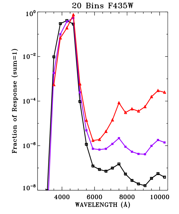
Figure 11: Fractional contribution to the WFC F435W signal in each of 20 bins spanning the full range of the filter transmission. Black is for the hot WD G191B2B, purple represents the K star KF06T2, and VB8 is red.

6.1 Alternatives to Bandpass Shifts

In order to explain the discrepant comparison of ACS photometry to STIS fluxes for cooler stars, Bohlin (2007) considered and dismissed alternatives to bandpass adjustments. In particular, out-of-band transmission errors are one alternative; and Figure 11 shows the contribution to the observed ACS photometric signal as a function of wavelength for F435W in 20 equal wavelength bins across the full measured range of the filter transmission. The fractional contributions are computed from the CALSPEC SEDs for a hot WD G191B2B, a K star KF06T2, and the M star VB8 using the ACS system throughput $R$. The central three bins contain $>$99% of the F435W signals for all three stars, while the bin on the short wavelength shoulder of the response contains most of the remaining contribution. As expected, the out-of-band red leak is more than an order of magnitude higher for the K star than for the WD in the 12 points longward of $\sim$5900 Å, while VB8 is another two orders of magnitude larger. However, these 12 bins for KF06T2 are $\sim 10^{-6}$ on average for a total red leak fraction of $\sim 10^{-5}$, which is a factor of 300 below the 0.3% tweak achieved by updating the F435W filter edge shift from +18 to +21 Å. The ACS filter transmissions were all carefully measured in the lab before launch and have exellent out-of-band rejections. Bohlin (2007) showed a similar figure for F625W; and all results for all eight of the broadband filters are similar, with total red+blue leaks of $<10^{-4}$, i.e. $<0.01\%$ for K and hotter stars. The transmission of F850LP was not measured longward of the CCD QE cutoff of 11000 Å.

7 Absolute Flux Calibration

7.1 Adjustments for Individual Filters

Following any correction for filter bandpass shifts, the average residual deviation of C/P from unity is corrected by multiplying each filter transmission by the average residual in order to correct the P values that are computed from the total system QE, i.e. $R$, which is the product of the throughput of all the HST+ACS mirrors, the filter transmission, and the detector QE. The C values are for the 1″ (20 pixel) photometry from the *_crj.fits files, as corrected for the pixel area maps (PAMs), the CTE losses, and the EE. Table 6 contains these average C/P residuals; and Figure 12 shows the final WFC average values (squares) for the three primary WDs at unity with the cooler stars shown as colored symbols. There is no consistent significant trend of the corrections with wavelength that would mandate an update of the detector QE functions. The new filter throughputs include the correction for these residuals, which are then propagated to the final $photflam$ values according to Equation 3.

The fully corrected photometry for the F, G, and K stars in the eight broadbands in Figure 12 is within the goal of 1% agreement, except for one measure of the variable star BD+17^∘4708, which is consistently low in all eight broadbands. The variable BD+17^∘4708 (Bohlin & Landolt, 2015) is observed at different epochs for the ACS numerator values and the STIS denominator. The sub-percent internal consistency shown in Figure 12 is achieved for the first time and is indicative of the consistency of the revised ACS flux calibration relative to STIS (B14).

Table 6: Filter Transmission Updates

	Residuals
Filter	WFC	3$\sigma$	HRC	3$\sigma$
F220W	…	…	0.988	0.005
F250W	…	…	0.990	0.005
F330W	…	…	0.991	0.003
F344N	…	…	0.992	0.005
F435W	1.001	0.002	0.992	0.003
F475W	1.003	0.002	0.996	0.004
F502N	1.001	0.003	0.997	0.007
F555W	1.004	0.002	0.998	0.001
F550M	1.000	0.002	0.995	0.005
F606W	1.006	0.002	1.000	0.002
F625W	1.006	0.002	0.999	0.004
F658N	1.007	0.003	1.003	0.009
F660N	1.018	0.007	1.010	0.008
F775W	1.008	0.002	1.001	0.001
F814W	0.994	0.002	1.000	0.003
F892N	1.006	0.004	1.015	0.009
F850LP	1.008	0.002	1.007	0.005

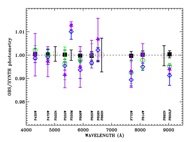
Figure 12: C/P count rate ratios vs. pivot wavelength for the stars observed with WFC after making the corrections for the F435W and F814W filter shift and the corrections in Table 6 for the filter transmissions. The black squares for the average of the three prime WDs are now all within 0.001 of unity, while the averages and 3$\sigma$ errors-in-the-mean are shown for the F (blue diamond), G (green circle), and K (purple star) standards. The less precise results for the sparsely observed narrow and medium band filters are the open black squares.

7.2 Uncertainty in the Flux Calibration

7.2.1 Uncertainty at WFC1-1K

The ACS absolute flux calibrations $S$ are computed with the system QE, i.e. $R$, according to Equation 3, where the $R$ functions are determined from C/P, as in Section 7.1. Because the infinite aperture count rate C is computed from the 20 pixel aperture photometry that has the best repeatability as $C=N_{20}/E_{20}$, the uncertainty in $S$ is the uncertainty in the average $N_{20}/E_{20}$, where the repeatability of $N_{20}$ from Table 3 for the broadband WFC filters is 0.30–0.53% for the 20 pixel radius photometry. The uncertainty in the average $N_{20}$ rms scatter is reduced by the typical number of 23 broadband observations of the primary WDs to a maximum of $0.53/\sqrt{23}=0.11~{}\%$, while the uncertainty for $E_{20}$ from Section 4.3 is 0.1%. Thus, the formal uncertainties in the ACS broadband $photflam$ values that are based on the 20 pixel radius photometry are all $\leq$0.15%. For the four narrow band filters, the statistical measurement uncertainties are somewhat larger according to their error bars in Figure 12.

However, this systematic uncertainty increases, if smaller aperture photometry is required. For example, the maximum of 2.23% from Table 3 for F775W combined with the EE uncertainty of 0.4% makes a total WFC three pixel flux calibration systematic error of $\sqrt{{2.23^{2}}/23+0.4^{2}}=0.6\%$, which has a floor value of 0.4%, even if the ACS observational data set were greatly increased. The EE uncertainty is not likely to benefit significantly from more observations, as that 0.4% is already based on a smooth fit to a large data set.

The above error estimates are relative to the STIS flux calibration that determines the $P$ values in C/P, and the external STIS uncertainties are presented in figure 14 of B14. Thus, the systematic ACS and STIS errors must be combined to get the full systematic uncertainty. For example, the STIS uncertainty at the 9033 Å pivot wavelength of F850LP is 0.4% relative to the reference wavelength of 5556 Å. Combining the STIS 0.4% with the ACS WFC uncertainties of 0.87/$\sqrt{23}$ from Table 3 and 0.2% in EE for a five pixel radius makes a total of $\pm$0.5% for F850LP relative to 5556 Å. A grand total absolute uncertainty should also include the 0.5% uncertainty in the reference flux for Vega at 5556 Å (Bohlin, 2014). A proper formal STIS error analysis should utilize the covariant matrix $WDcovar.fits$ from B14 that is available in the CALSPEC archive.

7.2.2 Uncertainty around the Full Field of View

If the flat fields were perfect for stars of any spectral type. then the above discussion of uncertainties at the WFC1-1K reference point would apply everywhere. However, there are sometimes problems with flat field uniformity, as discussed in Bohlin & Grogin (2015) and in Sections 4.5 and 6 above. While the bandpass adustments of Section 6 brings the uniformity to better than 1% for F814W, F435W shows larger variations of -2 to +3% in GD153-KF06T2 differential photometry. The throughput variations around the F435W FOV for the individual stars are -4.2 to +1.7% for the WD and -2.7 to +0.9% for the K star. The existing flat fields are all based on the average stellar type in 47 Tuc (Mack et al., 2002); and the smaller error range for the K star KF06T2 suggests that the average type of 47 Tuc is closer to K than to the 40,000 K WD GD153. In the presence of flat fielding errors, the absolute flux calibrations provided here for the hot WDs at the WFC1-1K reference point may differ somewhat from an average over the full field; but there is now at least one point where the calibration is fully characterized. If the -4.2 to +1.7% WD error range for F435W is a worst case, then -1.2% would be the largest systematic error of the WFC1-1K calibraton with respect to the FOV average. Except for F435W and F814W, there is little data on flat fielding errors for stars that differ from the mean color of the 47 Tuc stars that define the flat fields. However, Bohlin (2012) demonstrated that the meager archival photometry for F775W varied by $<$0.5% for the WD G191B2B at seven different positions in the FOV.

7.3 QE Reference Files

The changing ACS sensitivity is incorporated in the pipeline data processing via the Synphot QE reference files for the WFC and HRC CCD detectors, which are structured with wavelength in column 1, a default QE in column 2 for unspecified dates, and then pairs of QE columns, where the actual QE at any date is linearly interpolated in time between the dates for columns 3 and 4, columns 5–6, etc. The $photflam$ calibration constants $S$ in the ACS data headers are computed for the time of the observation using the new QE reference files acs_hrc_ccd_mjd_016_syn.fits or the pair of identical WFC files: acs_wfc_ccd1_mjd_022_syn.fits and acs_wfc_ccd2_mjd_022_syn.fits.

This calibration scheme is reflected in Table 7, where the default column 2 in the reference file is omitted; and the photflam values are those calculated using the QE vectors for the dates of the columns in the QE reference files. In the case of HRC, there is only one pair of QE columns with dates of 2002.16 and the end of HRC operations at 2007.1 (MJD=54136).

For WFC, the QE changed at 2006.5 with the switch to the side 2 electronics chain when the operating temperature was lowered, so that the first pair of QE columns for -77C cover the date range 2002.16–2006.5 (MJD 52334–53919), while the second pair for -81C is for 2006.5–2009.4 (MJD 53920–54976); and the third pair covers 2009.4–2021.0 (MJD 54977–59214). The loss rates for the first two pairs of WFC columns through 2009.4 and for HRC are those specified in Table 5, while the difference between the WFC columns for 2009.4–2021.0 represents the average post-SM4 loss rate of 0.061%/yr. The ACS CCD channels were inactive from early 2007 until after the SM4 servicing mission at 2009.4, i.e. MJD 54977; but defining a correction during this dead time causes no harm.

The QE of the HRC detector at 2002.16 in the reference file was updated by Bohlin (2012), but the WFC QE was last adjusted by Bohlin (2007). Thus, the changes from the previous calibration for the 2002.16 photflam values in Table 7 are due only to the filter residuals of Table 6 and to the two WFC bandpass adjustments. The differences between columns 3 and 4 in the Table 7 $photflam$ values represent the change from the set point temperature of -77C to -81C at 2006.5 (Mack et al., 2007), while the differences from column 2 to column 6 at 2009.4 include both the Mack et al. (2007) adjustment for the colder temperature and the adjustments in final column of Table 5. The second value of each pair represents the increased photflam that compensates for the loss in sensitivity from the date of the first photflam of the pair.

The infinite aperture $photflam$ calibrations of Table 7 are included in the ACS data headers but must be converted for practical usage of smaller aperture photometry via Equation 1, where $\langle F\rangle={S~{}N_{e}}=S~{}N_{i}/E_{i}$. N_i is photometry for the $ith$ aperture radius and $E_{i}$ is the encircled energy EE correction from Table 8 or Table 9. In case such a table for any future revision is not at hand or to avoid the necessity of consulting the literature to calibrate aperture photometry, the $photflam(i)=S/E_{i}$ or just the $E_{i}$ should also be included in the $fits$ data headers for the i=3, 5, 10, and 20 aperture radii.

7.4 Implications of Updated Calibration

New data contributes to improved mean EE values, which are now provided for aperture radii as small as one pixel. The robust set of new post-SM4 data reveals a sensitivity loss for all filters of 0.061%/yr, so that by 2017, the change in sensitivity will reach 0.5% from the time of the 2009 SM4. Another new body of data for F435W and F814W demonstrates the need for small bandpass adjustments for those two filters.

Column 2 for WFC or column 8 for HRC in Table 7 can be compared to the $photflam$ results of Sirianni et al. (2005) for the first years of ACS operations. The current WFC values range from 5% smaller for F660N to 1% larger for F550M, while the eight broadband filters are 1–3% smaller. For HRC, differences range from 0–3% smaller, except for F344N, where the new calibration is 3% larger. These differences are due mostly to changes in the CALSPEC reference SEDs and to a refined and expanded set of ACS observations of these standard stars. Sirianni et al. (2005) utilized many observations of GRW+70^∘5824, which has a poor, noisy CALSPEC SED that can affect the synthetic photometry, especially for narrow bandpasses. Observations of GRW+70^∘5824 are not used for the current, new $photflam$ results in Table 7.

Table 7: ACS infinite aperture calibration constants $photflam$, i.e. $S$ in units of $erg~{}s^{-1}~{}cm^{-2}~{}\AA^{-1}/(e~{}s^{-1})$. The applicable dates are listed as MJD and as fractional year, along with the WFC CCD set point temperature. The $S$ at any date is the linear interpolation between pairs of columns.

	WFC							HRC
Filter	MJD52334	MJD53919	MJD53920	MJD54976	MJD54977	MJD59214		MJD52334	MJD54136
	2002.16	2006.5	2006.5	2009.4	2009.4	2021.0		2002.16	2007.1
	-77C	-77C	-81C	-81C	-81C	-81C
F220W								8.063e-18	8.333e-18
F250W								4.636e-18	4.731e-18
F330W								2.210e-18	2.235e-18
F344N								2.200e-17	2.222e-17
F435W	3.062e-19	3.082e-19	3.155e-19	3.169e-19	3.135e-19	3.157e-19		5.318e-19	5.358e-19
F475W	1.781e-19	1.793e-19	1.828e-19	1.837e-19	1.819e-19	1.832e-19		2.884e-19	2.907e-19
F502N	5.131e-18	5.168e-18	5.257e-18	5.283e-18	5.237e-18	5.274e-18		7.977e-18	8.043e-18
F550M	3.906e-19	3.939e-19	3.991e-19	4.013e-19	3.973e-19	4.002e-19		5.797e-19	5.851e-19
F555W	1.920e-19	1.935e-19	1.964e-19	1.974e-19	1.955e-19	1.969e-19		2.985e-19	3.012e-19
F606W	7.666e-20	7.728e-20	7.824e-20	7.867e-20	7.778e-20	7.834e-20		1.258e-19	1.270e-19
F625W	1.168e-19	1.178e-19	1.191e-19	1.197e-19	1.183e-19	1.191e-19		1.942e-19	1.960e-19
F658N	1.940e-18	1.956e-18	1.976e-18	1.988e-18	1.962e-18	1.976e-18		3.320e-18	3.352e-18
F660N	5.077e-18	5.120e-18	5.172e-18	5.201e-18	5.134e-18	5.171e-18		8.754e-18	8.838e-18
F775W	9.826e-20	9.878e-20	1.000e-19	1.004e-19	9.912e-20	9.983e-20		1.926e-19	1.938e-19
F814W	6.943e-20	6.974e-20	7.082e-20	7.103e-20	7.017e-20	7.067e-20		1.268e-19	1.274e-19
F850LP	1.489e-19	1.493e-19	1.528e-19	1.531e-19	1.514e-19	1.525e-19		2.247e-19	2.254e-19
F892N	1.475e-18	1.479e-18	1.510e-18	1.512e-18	1.496e-18	1.506e-18		2.436e-18	2.443e-18

8 Conclusions and Recommendations

For stellar types of K and hotter, Figure 12 demonstrates the achievement of the goal of 1% precision of the ACS/WFC flux calibration relative to the STIS standard stars for the eight well observed broadband filters. Small adjustments of the filter transmission functions for F555W, F775W, and F850LP similar to those for F435W and F814W would bring the agreement for all eight filters within 0.5% at the WFC1-1K reference point; but before making those three new transmission corrections, confirming observations should be obtained like those mapping the FOV for F435W and F814W.

If precision photometry of the coolest stars of type M and later is important, then the WFC calibration for these types could be improved by more observations both with ACS/WFC and STIS. Action to augment the header keywords, to solve the drizzle problem, and to derive color dependent F435W flat fields is not yet scheduled. However, the new photflam flux calibration should be implemented by the time this article is published. The photflam data header keyword for the infinite aperture includes the changes with time of Section 5, which are encapsulated in the reference files acs_hrc_ccd_mjd_016_syn.fits and acs_wfc_ccd*_mjd_022_syn.fits, where the asterisk can be either of the identical 1 or 2 files. The revised filter throughput curves are named by filter and detector and are also available as reference files, while EE values must be read from Tables 8 and Table 9 herein.

ACKNOWLEDGEMENTS

Thanks to J. Mack for re-drizzling the jcr601081_drz.fits image and for suggesting that the WHT drizzle extent can be used to distinguish between good and bad drz photometry. Wayne Landsman provided the IDL photometry routine apphot.pro. This research has made use of the SIMBAD database, operated at CDS, Strasbourg, France.

Appendix A Drizzle $drz$ Photometry

In principle, extracting photometry from the geometrically corrected drizzled *_drz.fits files is more straightforward than using the *_crj.fits files. There is no need to apply PAMs and the plate scale is constant at exactly 0.05″ per pixel for WFC (0.025″ for HRC). However, the *_drz.fits files are problematic when combining pairs of images; and use of the default pipeline products requires extreme caution. The second extention of the drz product is the weight (WHT) image, which offers clues to the drizzle validity. If the pair of *_flt.fits images that are combined into the drz have slightly different or misaligned PSFs or even mis-matched backgrounds (Avila et al., 2015), a reduced WHT coincident with the core of the star usually indicates improper cosmic-ray flagging. A data quality (DQ) parameter can be defined as the percent drop from maximum to minimum WHT weight in the 3x3 set of pixels centered on the star. Setting a DQ=13.1% limit provides a fairly good dividing line between good and bad drz photometry for pairs of images, and most of the errors are flagged without flagging many of the valid drz results. The crj photometry is validated by the small $\sigma_{20}<$0.5% in Table 3 for the baseline 20 pixel photometry.

Figure 13, compares the WFC drz with the baseline crj 1″ photometry of the standard stars as a function of the response in the peak pixel of each observation. There are 239 unflagged comparisons shown as the filled circles that are all within 1% of perfect agreement. However, the 95 flagged ratios are 28% of the total, are usually in error by more than 1%, and occassionally are in error by more than a factor of two. The crj pipeline product from the MAST data archives is not always perfect, even for the short standard star exposures, where hot pixels are not a problem. Of the 334 exposures in Figure 13, one (jcga02081_crj.fits) requires special re-processing with relaxed cosmic-ray (CR) rejection parameters, because the CR-split pair is slightly misaligned.

One case of combining the jcr601lhq and jcr601liq flt files to make the jcr601081 crj and drz files is investigated in detail. The pipeline drz/crj photometry ratio is 0.91, while the peak is 79000 (open red circle in Figure 13). Reprocessing this observation with relaxed drizzle constraints for cosmic-ray rejection of driz_cr_scale=(1.5, 1.2), instead of the pipeline default (1.2, 0.7) values (Gonzaga et al., 2012) produces a revised ratio of unity (filled red circle in Figure 13). The ACS drizzle product could be much more useful to the science community by a relaxation of the pipeline parameters that would bring drz photometry into agreement with the robust crj results.

Figure 13: Comparison of 20 pixel photometry from crj and drz files for the WFC standard star observations. The 239 filled black circles are the ratios for drz photometry with good weight (WHT) arrays, while the open black circles represent the same ratio but with a WHT DQ parameter of greater than 0.131. The erroneous drz results become more frequent above a peak signal level of about half of the CCD saturation level of 83,000 electrons. The open and filled red circles represent pipeline processing and a special reprocessing with relaxed drizzle constrains, respectively, which suggests that the default pipeline drizzle parameters could be improved.

The ACS/CCD flux calibrations at the WFC1-1K reference point for the good, unflagged WFC drz photometry are equivalent to the crj calibrations, except for the small, three pixel radius, where the drz photometry and EE are systematically $\sim$0.5% smaller. The average 1″ (20 pixel) drz photometry for the three WDs is the same as the crj results within 0.1%; and the drz flux calibration is the same as the crj calibration in Table 6 to 0.1%. Except for the 0.5% difference for the three pixel radius, any systematic difference between drz and crj WFC photometry at the WFC1-1K reference point is less than the uncertainty; and the crj calibration is accurate for drz results. At other locations in the FOV, the sparse data set combined with the problematic drz results prohibit reliable measures of any differences between drz and crj EE.

Appendix B Encircled Energies

Table 8 and Table 9 include EE values for 12 aperture radii as computed according to the quartic fitting procedure of Section 4.3.

Table 8: Encircled Energy Fractions for Hot Stars at WFC1-1K

Filter	1 pix	2 pix	3 pix	4 pix	5 pix	6 pix	7 pix	8 pix	9 pix	10 pix	20 pix	40 pix
F435W	0.330	0.663	0.792	0.839	0.863	0.877	0.887	0.895	0.902	0.907	0.941	0.979
F475W	0.329	0.670	0.794	0.842	0.868	0.883	0.893	0.901	0.907	0.912	0.944	0.979
F502N	0.328	0.670	0.794	0.842	0.869	0.884	0.894	0.902	0.909	0.914	0.945	0.978
F555W	0.328	0.668	0.794	0.841	0.868	0.885	0.895	0.903	0.910	0.915	0.946	0.977
F550M	0.328	0.666	0.794	0.840	0.867	0.885	0.896	0.904	0.910	0.915	0.947	0.976
F606W	0.328	0.661	0.795	0.839	0.866	0.885	0.896	0.904	0.910	0.916	0.947	0.975
F625W	0.330	0.655	0.795	0.838	0.864	0.884	0.896	0.904	0.911	0.916	0.948	0.974
F658N	0.331	0.651	0.794	0.838	0.863	0.883	0.896	0.904	0.911	0.916	0.948	0.973
F660N	0.331	0.650	0.794	0.838	0.863	0.883	0.896	0.904	0.911	0.916	0.948	0.973
F775W	0.329	0.625	0.783	0.836	0.858	0.877	0.894	0.904	0.910	0.916	0.949	0.972
F814W	0.322	0.611	0.770	0.830	0.853	0.871	0.889	0.901	0.908	0.914	0.949	0.972
F892N	0.278	0.546	0.705	0.787	0.818	0.840	0.860	0.877	0.889	0.897	0.942	0.970
F850LP	0.268	0.532	0.690	0.776	0.810	0.833	0.853	0.871	0.884	0.893	0.940	0.970

Table 9: Encircled Energy Fractions for Hot Stars at HRC Center

Filter	2 pix	4 pix	6 pix	8 pix	10 pix	12 pix	14 pix	16 pix	18 pix	20 pix	40 pix	80 pix
F220W	0.518	0.694	0.755	0.779	0.799	0.818	0.833	0.845	0.857	0.868	0.948	0.977
F250W	0.537	0.715	0.783	0.813	0.827	0.842	0.855	0.865	0.874	0.884	0.946	0.980
F330W	0.549	0.740	0.804	0.840	0.853	0.864	0.875	0.883	0.891	0.898	0.943	0.981
F344N	0.549	0.742	0.806	0.842	0.855	0.866	0.876	0.885	0.892	0.899	0.943	0.981
F435W	0.547	0.763	0.817	0.854	0.873	0.883	0.891	0.899	0.905	0.910	0.944	0.981
F475W	0.543	0.767	0.819	0.855	0.877	0.888	0.896	0.903	0.909	0.914	0.946	0.980
F502N	0.540	0.768	0.820	0.855	0.879	0.891	0.898	0.906	0.912	0.916	0.947	0.980
F555W	0.535	0.766	0.821	0.854	0.880	0.893	0.900	0.908	0.914	0.919	0.949	0.980
F550M	0.532	0.762	0.822	0.853	0.880	0.894	0.901	0.909	0.915	0.920	0.949	0.980
F606W	0.526	0.755	0.822	0.851	0.878	0.894	0.902	0.909	0.915	0.920	0.950	0.979
F625W	0.519	0.741	0.821	0.847	0.874	0.891	0.901	0.908	0.914	0.919	0.950	0.978
F658N	0.512	0.729	0.819	0.844	0.869	0.888	0.898	0.905	0.911	0.917	0.949	0.977
F660N	0.512	0.728	0.818	0.843	0.869	0.887	0.898	0.905	0.911	0.917	0.949	0.977
F775W	0.468	0.650	0.783	0.807	0.826	0.847	0.863	0.871	0.878	0.884	0.927	0.964
F814W	0.444	0.613	0.756	0.782	0.800	0.821	0.838	0.847	0.855	0.862	0.910	0.956
F892N	0.351	0.502	0.642	0.683	0.701	0.720	0.739	0.754	0.764	0.773	0.844	0.925
F850LP	0.333	0.484	0.619	0.664	0.682	0.700	0.720	0.736	0.746	0.756	0.831	0.919

References

- Anderson & Bedin (2010) Anderson, J., & Bedin, L. R. 2010, PASP, 122, 1035
- Avila et al. (2015) Avila, R. J., Hack, W., Cara, M., et al. 2015, in Astronomical Society of the Pacific Conference Series, Vol. 495, Astronomical Data Analysis Software an Systems XXIV (ADASS XXIV), ed. A. R. Taylor & E. Rosolowsky, 281
- Bohlin (2007) Bohlin, R. C. 2007, Photometric Calibration of the ACS CCD Cameras, Instrument Science Report, ACS 2007–06, (Baltimore: STScI), Tech. rep.
- Bohlin (2011) —. 2011, Flux Calibration of the ACS CCD Cameras II. Encircled Energy Correction, Instrument Science Report, ACS 2011–02, (Baltimore: STScI), Tech. rep.
- Bohlin (2012) —. 2012, Flux Calibration of the ACS CCD Cameras IV. Absolute Fluxes, Instrument Science Report, ACS 2012–01, (Baltimore: STScI), Tech. rep.
- Bohlin (2014) —. 2014, AJ, 147, 127
- Bohlin & Anderson (2011) Bohlin, R. C., & Anderson, J. 2011, Flux Calibration of the ACS CCD Cameras I. CTE Correction, Instrument Science Report, ACS 2011–01, (Baltimore: STScI), Tech. rep.
- Bohlin et al. (2014) Bohlin, R. C., Gordon, K. D., & Tremblay, P.-E. 2014, PASP, 126, 711 (B14)
- Bohlin & Grogin (2015) Bohlin, R. C., & Grogin, N. 2015, Flat Field Determinations using an Isolated Point Source, Instrument Science Report, ACS 2015–07, (Baltimore: STScI), Tech. rep.
- Bohlin & Landolt (2015) Bohlin, R. C., & Landolt, A. U. 2015, AJ, 149, 122
- Bohlin et al. (2011) Bohlin, R. C., Mack, J., & Ubeda, L. 2011, Flux Calibration of the ACS CCD Cameras III. Sensitivity Changes over Time, Instrument Science Report, ACS 2011–03, (Baltimore: STScI), Tech. rep.
- Bohlin & Proffitt (2015) Bohlin, R. C., & Proffitt, C. R. 2015, Improved Photometry for G750L, Instrument Science Report, STIS 2015–01, (Baltimore: STScI), Tech. rep.
- Gilliland (2004) Gilliland, R. L. 2004, ACS CCD Gains, Full Well Depths, and Linearity up to and Beyond Saturation, Instrument Science Report ACS 2004–01, (Baltimore: STScI), Tech. rep.
- Gilliland et al. (2006) Gilliland, R. L., Bohlin, R., & Mack, J. 2006, WFC L-Flats Post Cooldown, Instrument Science Report, ACS 2006–06, (Baltimore: STScI), Tech. rep.
- Gonzaga et al. (2012) Gonzaga, S., Hack, W., Fruchter, A., & Mack, J. 2012, The DrizzlePac Handbook, (Baltimore:STScI)
- Grogin et al. (2010) Grogin, N. A., Lim, P. L., Maybhate, A., Hook, R. N., & Loose, M. 2010, in Hubble after SM4. Preparing JWST, Post-SM4 ACS/WFC Bias Striping: Characterization And Mitigation, 2010 STScI Calibration Workshop, eds. S. Deustua and C. Oliveira (Baltimore: STScI), 481
- Krist & Hook (2004) Krist, J., & Hook, R. 2004, The Tiny Tim User’s Guide, Version 6.3 (Baltimore: STScI) http://www.stsci.edu/software/tinytim, p. 8, Tech. rep.
- Mack et al. (2002) Mack, J., Bohlin, R., Gilliland, R., et al. 2002, ACS L-Flats for the WFC, Instrument Science Report, ACS 2002–08, (Baltimore:STScI), Tech. rep.
- Mack et al. (2007) Mack, J., Gilliland, R. L., Anderson, J., & Sirianni, M. 2007, WFC Zeropoints at -80C, Instrument Science Report, ACS 2007–02, (Baltimore:STScI), Tech. rep.
- Scolnic et al. (2014) Scolnic, D., Rest, A., Riess, A., et al. 2014, ApJ, 795, 45
- Sirianni et al. (2005) Sirianni, M., Jee, M. J., Benítez, N., et al. 2005, PASP, 117, 1049 (S05)
- Stys et al. (2004) Stys, D. J., Bohlin, R. C., & Goudfrooij, P. 2004, Time-Dependent Sensitivity of the CCD and MAMA First- Order Modes, Instrument Science Report, STIS 2004–04, (Baltimore:STScI), Tech. rep.
- Ubeda & Anderson (2013) Ubeda, L., & Anderson, J. 2013, Study of the evolution of the ACS/WFC Sensitivity Loss, Instrument Science Report, ACS 2013–01, (Baltimore: STScI), Tech. rep.