ROCS-Derived Features for Virtual Screening

Abstract

Rapid overlay of chemical structures (ROCS) is a standard tool for the calculation of 3D shape and chemical (“color”) similarity. ROCS uses unweighted sums to combine many aspects of similarity, yielding parameter-free models for virtual screening. In this report, we decompose the ROCS color force field into color components and color atom overlaps, novel color similarity features that can be weighted in a system-specific manner by machine learning algorithms. In cross-validation experiments, these additional features significantly improve virtual screening performance (ROC AUC scores) relative to standard ROCS.

1 Introduction

Ligand-based virtual screening is based on the assumption that similar compounds have similar biological activity [willett2009similarity]. Compound similarity can be assessed in many ways, including comparisons of molecular “fingerprints” that encode structural features or molecular properties [todeschini2009molecular] and measurements of shape, chemical, and/or electrostatic similarity in three dimensions [hawkins2007comparison; muchmore2006use; ballester2007ultrafast]. Three-dimensional approaches such as rapid overlay of chemical structures (ROCS) [hawkins2007comparison] are especially interesting because of their potential to identify molecules that are similar from the point of view of a target protein but dissimilar in underlying chemical structure (“scaffold hopping”; [bohm2004scaffold]).

ROCS represents atoms as three-dimensional Gaussian functions [grant1995gaussian; grant1996fast] and calculates similarity as a function of volume overlaps between alignments of pre-generated molecular conformers. Chemical (“color”) similarity is measured by overlaps between dummy atoms marking interesting chemical functionalities: hydrogen bond donors and acceptors, charged functional groups, rings, and hydrophobic groups. For simplicity, the shape and color similarity scores are typically combined into a single value that can be used to rank screening molecules against query molecules with known activity. If more than one query molecule is available, scores relative to each query can be combined using simple group fusion methods such as max [chen2010combination].

Machine learning methods offer powerful alternatives to combined similarity scores and group fusion when additional experimental data is available for training. By learning system-specific weights for the combination of similarity features, these methods can avoid the loss of information that results from combining these features arbitrarily (e.g., with an unweighted sum). For example, sato2012application showed that support vector machines (SVMs) trained on ROCS similarity to a set of query molecules outperformed simple group fusion models. Separating ROCS shape and color similarity scores and allowing the model to weight them independently resulted in additional performance gains.

In this report, we extend the reductionism of sato2012application by decomposing ROCS color similarity scores into (1) separate components for each color atom type (color components) and (2) individual scores for color atoms in query molecules (color atom overlaps). We demonstrate significant gains in virtual screening performance for machine learning models trained on these features compared to standard ROCS and simpler partitioning of shape and color similarity scores.

2 Methods

2.1 ROCS features

All features were based on pairwise calculations by rapid overlay of chemical structures (ROCS) [rocs]. ROCS measures the shape and chemical (“color”) similarity of two compounds by calculating Tanimoto coefficients from aligned overlap volumes:

$$\text{T}\left(A,B\right)=\frac{O_{AB}}{O_{AA}+O_{BB}-O_{AB}},$$ (1)

where $O_{AB}$ is the aligned overlap volume between molecules $A$ and $B$. Color similarity is calculated from overlaps between dummy atoms marking a predefined set of pharmacophore features defined by the ROCS color force field. The shape and color Tanimoto scores are often combined using an unweighted sum or average to give a single similarity measure, TanimotoCombo. In typical ROCS usage, one molecule is used as a reference or query to search a screening database or library for similar compounds.

An alternative similarity measure, reference Tversky, emphasizes overlap with the query molecule:

$$\text{Tv}\left(A,B\right)=\frac{O_{AB}}{\alpha O_{AA}+\left(1-\alpha\right)O_{BB}},$$ (2)

where molecule A is the query and $\alpha$ varies the bias of the measurement toward the query. In this report we used $\alpha=0.95$.

ROCS alignments, shape and color overlap volumes, and Tanimoto scores were calculated using the OEBestOverlay object in the oeshapetk (version 1.10.1). Overlays used the default Implicit Mills-Dean color force field, OEOverlapRadii_All, OEOverlapMethod_Analytic, and the following additional parameters: color_opt=True, use_hydrogens=False, all_color=True.

2.1.1 Color components

The default color force field defines six color atom types—hydrogen bond donors and acceptors, cations, anions, rings, and hydrophobes—and the volume overlap terms use to calculate color Tanimoto scores are unweighted sums of the overlap volumes for each color type. Since some pharmacophore types may be more important than others in individual systems, we calculated separate similarity scores for each color atom type. These scores are referred to as ROCS color components.

2.1.2 Color atom overlaps

In systems where query molecules have more than a single color atom of a given type, ROCS color similarity scores do not contain information about the relative locations of pharmacophore features. For example, a query molecule with two hydrogen bond acceptors may give suboptimal color similarity scores for library molecules if only one acceptor is important for activity. To avoid this problem and allow models to distinguish between individual color features, we calculated overlaps for individual color atoms in query molecules. These features are referred to as ROCS color atom overlaps.

The ROCS features used in this report, including color components and color atom overlaps, are depicted in Figure 1. We note that the values used to calculate color components and color atom overlaps are available internally to ROCS, but they are not directly accessible with the Shape Toolkit.

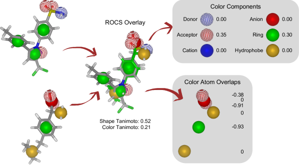
Figure 1: Molecular descriptors based on the ROCS color force field. Color components represent each color type independently. Color atom overlaps describe similarity in terms of individual color atoms in the query molecule (bottom left). Color component values are Tanimoto scores, but other similarity metrics—such as reference Tversky—could be used as well. Note that color atom overlap volumes are used without normalization, and that negative values indicate favorable interactions.

2.2 Datasets

We report results on three dataset collections with varying degrees of difficulty. First, the enhanced directory of useful decoys (DUD-E) contains 102 datasets designed for validation of structure-based virtual screening methods [mysinger2012directory]. Each dataset has an associated protein structure and bound ligand. Second, the maximum unbiased validation (MUV) collection contains 17 datasets designed for validation of ligand-based virtual screening methods [rohrer2009maximum]. Each dataset contains a set of maximally distinct actives individually embedded in a set of decoy molecules to avoid analog bias and artificial enrichment. The third dataset collection was derived from ChEMBL [gaulton2012chembl] for validation of ligand-based methods [riniker2013open; riniker2013heterogeneous]. Each dataset (80 in total) contains a set of diverse actives and shares a common set of decoys.

Up to 50 conformers for library molecules were generated with OpenEye OMEGA [hawkins2010conformer; omega]. Query molecules were either used as given (DUD-E crystal ligands) or with a single OMEGA conformer (DUD-E, MUV, and ChEMBL).

By default, OMEGA does not generate conformers for molecules with unspecified stereochemistry at chiral centers. This resulted in many compounds failing the conformer generation step and consequently being excluded from our experiments. Notably, 12 DUD-E crystal ligands failed OMEGA expansion and the corresponding datasets were removed from the collection entirely, reducing this collection to 90 datasets. Additionally, about half of all ChEMBL compounds (actives and decoys) failed conformational expansion due to unspecified stereochemistry.

The datasets in our collection are listed in Section A, along with counts of active and decoy molecules (not including OMEGA failures).

2.3 Machine learning

Standard ROCS is a parameter-free model that assigns the TanimotoCombo or other combined similarity score relative to a query molecule as the positive class probability. In situations where more than one query molecule is available, group fusion methods such as max can be used to combine multiple similarity scores into a single predicted value [chen2010combination]. However, if more than one feature is used to describe similarity or when more sophisticated combinations of multi-query similarities are desired, machine learning or other statistical approaches can be used to learn appropriate weights for each feature and tune performance for specific systems.

Given a training set of $n$-dimensional feature vectors $\left\{\bm{x_{1}},\bm{x_{2}},\dots,\bm{x_{m}}\right\}$ with corresponding class labels $\left\{y_{1},y_{2},\dots,y_{m}\right\}\in\left\{0,1\right\}$, a binary classifier learns a decision function that predicts the positive class probability $\hat{y}$ of an unlabeled feature vector $\bm{\hat{x}}$. The feature vectors are representations of the input examples, encoding information that the classifier will attempt to correlate to the output labels. Here, we use ROCS similarity scores and other values derived from ROCS as features describing the relationships between query and library molecules. For example, to learn system-specific weights for combining shape and color Tanimotos relative to a single query, we would construct feature vectors containing two elements corresponding to the separated shape and color Tanimoto scores.

In this work, we trained three different types of binary classifiers: logistic regression (LR), random forest (RF), and support vector machine (SVM). Logistic regression is a simple linear classifier: a weight is assigned to each feature and the output of the model is a biased linear combination of the input features which is then nonlinearly scaled to the range $[0,1]$. Random forest is an ensemble method which averages the output from several decision trees trained on subsets of the input data [svetnik2003random]. Support vector machines are maximum-margin classifiers that can model nonlinear relationships with the appropriate choice of kernel function.

Classifiers were trained using scikit-learn 0.17.1 [pedregosa2011scikit]. Model hyperparameters ($C$ for LR and SVM) were tuned by stratified cross-validation on training data. RF models used 100 trees and SVM models used the RBF kernel. All models used the ‘balanced’ class weighting strategy. We also increased the maximum number of iterations for LR models to $10\,000$.

2.4 Model training and evaluation

Models were trained using features calculated with respect to a single query molecule using 5-fold stratified cross-validation and evaluated using metrics calculated from the receiver operating characteristic (ROC) curve [fawcett2006introduction]. The area under the ROC curve (AUC) is a global measure of classification performance. ROC enrichment ($E_{x}$) measures performance early in the ranked list of library molecules, calculated as the ratio of the true positive rate (TPR) and the false positive rate (FPR) at a specific FPR [jain2008recommendations]. We calculated ROC enrichment at four FPR values: 0.005, 0.01, 0.02, and 0.05. The TPR corresponding to each FPR was estimated by interpolation of the ROC curve generated by the roc_curve method in scikit-learn [pedregosa2011scikit].

For each metric, we calculated mean test set values for each dataset across all cross-validation folds. Per-dataset 5-fold mean metrics were further summarized as medians within dataset collections (DUD-E, MUV, or ChEMBL) and differences between methods are reported as median per-dataset $\Delta$AUC or $\Delta E_{x}$ (here, $\Delta$ indicates a difference between 5-fold mean values). Additionally, we report 95% Wilson score intervals for the sign test statistic. The sign test is a non-parametric statistical test that measures the fraction of per-dataset differences that are greater than zero, and the confidence interval is a measure of the expected consistency of an observed difference between two methods. To calculate these intervals, we used the proportion_confint method in statsmodels [seabold2010statsmodels] with alpha=0.05 and method=‘wilson’, ignoring any per-dataset differences that were exactly zero.

For the DUD-E datasets, we trained models with the provided crystal ligand as the query, using either the crystal coordinates or a single conformer generated with OMEGA, resulting in 180 models total (90 datasets times two query conformations). For each MUV and ChEMBL dataset, we trained 5-fold cross-validation models specific to each active compound. For example, a MUV dataset with 30 actives $\left\{a_{1},a_{2},\dots a_{30}\right\}$ resulted in 150 trained models corresponding to 30 rounds of 5-fold cross-validation, where the features for round $i$ were specific to $a_{i}$ (which was removed from the dataset before training).

When calculating median 5-fold mean AUC or ROC enrichment values and sign test confidence intervals, the $N_{i}$ 5-fold models for each MUV and ChEMBL dataset were treated as independent models rather than averaging across all queries. This strategy allowed for more direct comparisons between models trained on the same features and resulted in tighter confidence intervals than might be expected (since the number of observations is greater than the number of datasets). In total, we trained 378 5-fold models for MUV (17 datasets) and 4082 5-fold models for ChEMBL (80 datasets).

3 Results

3.1 Proof of concept: DUD-E

To assess the utility of color components and color atom overlaps features (see Section 2.1), we trained models on various combinations of input features using 5-fold cross-validation on the DUD-E datasets. All models used shape Tanimoto (ST) along with some variant of color similarity: color Tanimoto (CT), color component Tanimoto scores (CCT), and/or color atom overlaps (CAO). (Abbreviations for features are consolidated in Table 1.) Each DUD-E dataset has a crystal ligand that was used as the query molecule. As a comparative baseline, ROCS TanimotoCombo scores were used to rank test set molecules by similarity to the query; standard ROCS can be thought of as a model which assigns equal weight to the shape and color Tanimoto scores. Additionally, we trained models using a simple separation of shape and color similarity scores.

Table 1: Feature abbreviations.

Code	Description
ST	Shape Tanimoto
STv	Shape Tversky
CT	Color Tanimoto
CTv	Color Tversky
CCT	Color components (Tanimoto scores)
CCTv	Color components (Tversky scores)
CAO	Query molecule color atom overlaps

Table 2 shows median 5-fold mean AUC scores for DUD-E dataset models. For each model, we also report a two-sided 95% confidence interval around the mean difference in AUC relative to the ROCS baseline. ROC enrichment scores for these models are reported in Section C. (Note that our analysis in this report is based only on AUC scores.) In agreement with sato2012application, the ST-CT model achieved consistent improvements over ROCS by learning target-specific weights for the combination of these features. Replacing the color Tanimoto with color component scores (ST-CCT) gave an additional boost in performance, and using color atom overlaps (ST-CAO) yielded even greater improvement. Using color components and color atom overlaps in combination (ST-CCT-CAO) gave additional improvements for median AUC and/or $\Delta$AUC values, although these results were comparable to ST-CAO models (and were not always more consistent, as measured by sign test confidence intervals).

It is common practice to scale input features in order to improve model training and convergence. The results in Table 2 were produced without any feature scaling, but we experimented with two feature transformations: scaling by maximum absolute value and “standard” scaling by mean subtraction and division by the standard deviation (see Section B). Results for DUD-E crystal query models using these feature scaling strategies are reported in Table B.1 and Table B.2, respectively. Model performance was relatively insensitive to feature scaling, and our subsequent analysis is based on models trained without any feature transformations.

Table 2: Model performance on DUD-E datasets. We report median AUC, median per-dataset $\Delta$AUC, and a sign test 95% confidence interval (see Section 2.4) for models that used either the crystal ligand or a generated conformer as the query. Bold values indicate statistically significant confidence intervals that do not include 0.5.

		Crystal Query Conformer			Generated Query Conformer
Model	Features	Median AUC	Median $\Delta$AUC	Sign Test 95% CI	Median AUC	Median $\Delta$AUC	Sign Test 95% CI
white ROCS	TanimotoCombo	$0.697$			$0.633$
white	ST-CT	$0.729$	$0.023$	(0.72, 0.88)	$0.698$	$0.031$	(0.72, 0.88)
white	ST-CCT	$0.751$	$0.056$	(0.77, 0.91)	$0.730$	$0.074$	(0.79, 0.93)
white	ST-CAO	$0.813$	$0.123$	(0.92, 0.99)	$0.813$	$0.145$	(0.92, 0.99)
white LR	ST-CCT-CAO	$0.823$	$0.129$	(0.91, 0.99)	$0.825$	$0.158$	(0.92, 0.99)
white	ST-CT	$0.681$	$0.009$	(0.44, 0.64)	$0.678$	$0.031$	(0.52, 0.72)
white	ST-CCT	$0.811$	$0.124$	(0.89, 0.98)	$0.810$	$0.154$	(0.88, 0.98)
white	ST-CAO	$0.893$	$0.198$	(0.94, 1.00)	$0.888$	$0.231$	(0.94, 1.00)
white RF	ST-CCT-CAO	$0.893$	$0.211$	(0.94, 1.00)	$0.890$	$0.244$	(0.92, 0.99)
white	ST-CT	$0.754$	$0.052$	(0.82, 0.95)	$0.746$	$0.066$	(0.78, 0.92)
white	ST-CCT	$0.789$	$0.085$	(0.82, 0.95)	$0.778$	$0.110$	(0.83, 0.95)
white	ST-CAO	$0.864$	$0.167$	(0.94, 1.00)	$0.856$	$0.207$	(0.92, 0.99)
white SVM	ST-CCT-CAO	$0.869$	$0.171$	(0.94, 1.00)	$0.867$	$0.217$	(0.92, 0.99)

We considered the possibility that these results were skewed by the use of a crystal ligand as the query molecule. In most screening situations, a bioactive conformation of the query is not known, and it is possible that color components and color atom overlaps are more sensitive to the query conformation than standard ROCS. Accordingly, we used OMEGA to generate conformers for DUD-E crystal ligands and trained new models using generated conformers as queries; results for these models are shown in Table 2.

As expected, standard ROCS performance decreased relative to models trained using crystal query conformations (since generated conformers are not guaranteed to represent bioactive conformations). However, separating shape and color similarity or adding color components or color atom overlap features improved performance in a manner consistent with crystal conformer queries. Notably, many models achieved similar median AUC scores for both crystal and generated query conformers, suggesting that these models were less sensitive to the query conformation than standard ROCS.

3.2 Additional benchmarks

The DUD-E datasets were designed to avoid structural similarity between active and inactive molecules in order to reduce the potential for false negatives [mysinger2012directory]. Unfortunately, this aggravates issues such as artificial enrichment and analog bias [rohrer2009maximum] and limits their utility for validation of ligand-based methods [irwin2008community]. To increase confidence in our results, we trained models using ROCS-derived features on two additional dataset collections: the maximum unbiased validation (MUV) datasets of rohrer2009maximum and a group of benchmarking datasets derived from ChEMBL [riniker2013open; riniker2013heterogeneous], both of which were specifically designed for the validation of ligand-based methods. Since these datasets are not associated with specific reference molecules (such as crystal ligands), we trained multiple 5-fold models for each dataset using each active molecule as a query (see Section 2.4).

Performance metrics for models trained on MUV data are shown in Table 3. MUV is known to be an especially challenging benchmark, since each active molecule is explicitly separated from the others and is embedded among hundreds of decoys with similar properties, so it was not surprising that differences between MUV models were more variable and much smaller than the differences observed with DUD-E. RF models trained on MUV data were either no better or consistently worse than vanilla ROCS. The only models that significantly outperformed the ROCS baseline were trained on color atom overlap features, although sign test confidence intervals for these models indicated that the benefit of including these features was not as consistent for MUV as it was for DUD-E. ROC enrichment scores for these models are reported in Section C.

Results for models trained ChEMBL data are shown in Table 4. These datasets are more challenging than those in DUD-E, yielding a substantially lower median ROC AUC for the ROCS baseline (in fact, the ROCS median AUC for the ChEMBL datasets was lower than for MUV). In contrast to the results for MUV, all ChEMBL machine learning models saw consistent improvement over the ROCS baseline, with a ranking of feature subsets similar to that observed for the DUD-E datasets. Notably, the combination of color components and color atom overlaps (ST-CCT-CAO) resulted in substantial improvements in median AUC relative to ST-CAO features for LR and SVM models, although the sign test confidence intervals for these models were similar. ROC enrichment scores for these models are reported in Section C.

Table 3: Model performance on MUV datasets. We report median AUC, median per-dataset $\Delta$AUC, and a sign test 95% confidence interval (see Section 2.4). Several models were trained for each dataset, each using a different active molecule as the query. Bold values indicate statistically significant confidence intervals that do not include 0.5.

Model	Features	Median AUC	Median $\Delta$AUC	Sign Test 95% CI
white ROCS	TanimotoCombo	$0.586$
white	ST-CT	$0.603$	$0.001$	(0.46, 0.56)
white	ST-CCT	$0.599$	$0.002$	(0.46, 0.56)
white	ST-CAO	$0.615$	$0.037$	(0.58, 0.68)
white LR	ST-CCT-CAO	$0.632$	$0.042$	(0.60, 0.69)
white	ST-CT	$0.517$	$-0.059$	(0.25, 0.34)
white	ST-CCT	$0.545$	$-0.039$	(0.33, 0.43)
white	ST-CAO	$0.562$	$-0.005$	(0.43, 0.53)
white RF	ST-CCT-CAO	$0.566$	$0.000$	(0.45, 0.55)
white	ST-CT	$0.597$	$-0.002$	(0.44, 0.54)
white	ST-CCT	$0.591$	$0.003$	(0.47, 0.57)
white	ST-CAO	$0.609$	$0.035$	(0.56, 0.66)
white SVM	ST-CCT-CAO	$0.614$	$0.040$	(0.57, 0.67)

Table 4: Model performance on ChEMBL datasets. We report median AUC, median per-dataset $\Delta$AUC, and a sign test 95% confidence interval (see Section 2.4). Several models were trained for each dataset, each using a different active molecule as the query. Bold values indicate statistically significant confidence intervals that do not include 0.5.

Model	Features	Median AUC	Median $\Delta$AUC	Sign Test 95% CI
white ROCS	TanimotoCombo	$0.579$
white	ST-CT	$0.671$	$0.037$	(0.73, 0.76)
white	ST-CCT	$0.716$	$0.099$	(0.83, 0.86)
white	ST-CAO	$0.783$	$0.180$	(0.95, 0.96)
white LR	ST-CCT-CAO	$0.829$	$0.223$	(0.96, 0.97)
white	ST-CT	$0.617$	$0.032$	(0.59, 0.62)
white	ST-CCT	$0.744$	$0.142$	(0.85, 0.87)
white	ST-CAO	$0.821$	$0.213$	(0.95, 0.97)
white RF	ST-CCT-CAO	$0.834$	$0.224$	(0.96, 0.97)
white	ST-CT	$0.704$	$0.088$	(0.82, 0.85)
white	ST-CCT	$0.752$	$0.143$	(0.88, 0.89)
white	ST-CAO	$0.804$	$0.200$	(0.96, 0.97)
white SVM	ST-CCT-CAO	$0.835$	$0.227$	(0.96, 0.97)

3.3 Model interpretation

Color component and color atom overlap features provide fine detail on chemical features that can be correlated with biological activity. Accordingly, trained models can be interrogated for insights that are applicable to drug design. For example, the learned weights for individual color atom overlaps in a linear model contain information about the relative importance of those chemical features for activity.

There are some technical details to keep in mind for the examples that follow. Overlaps between color atoms are assigned negative feature values, such that negative weights for color atoms indicate features that are correlated with activity. Additionally, input features were not scaled during training or prediction; the default color force field uses the same parameters for each color atom interaction, such that learned weights for different color atoms should be directly comparable. Shape similarity feature values ranged from 0–1 (such that positive weights are correlated with activity); as such, shape and color similarity features were not guaranteed to be on the same scale.

Figure 2(a) depicts the learned color atom weights from a LR model trained on ST-CAO features for the DUD-E nram (neuraminidase) dataset using the crystal ligand as the query molecule. In this model, overlaps with the carboxylic acid anion, hydrophobic pentyl group, and the aromatic ring are most correlated with activity. Interestingly, overlaps with one of the carboxylic acid hydrogen bond acceptors are not favorable. LR models trained on ST-CAO features achieved a 5-fold mean AUC of $0.961$, compared to $0.862$ for standard ROCS.

As another example, Figure 2(b) shows color atom weights from a LR ST-CAO model for the DUD-E drd3 (dopamine receptor D3) dataset. The overlapping donor and cation color atoms (lower right) are assigned positive and negative weights, respectively. These weights suggest a potentially counterintuitive result, that overlap with the query cation is important for activity while the presence of a hydrogen bond donor at the same location is correlated with inactivity. LR ST-CAO models substantially outperformed vanilla ROCS on this dataset ($0.841$ vs. $0.313$ 5-fold mean AUC).

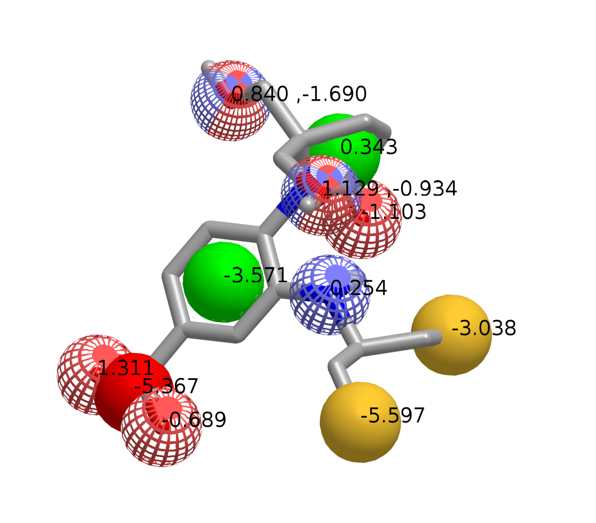
(a) ST weight = $2.492$

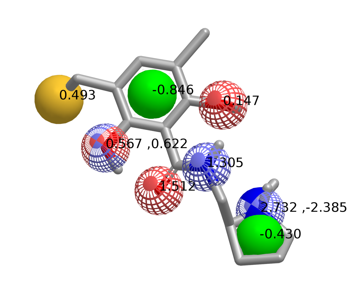
(b) ST weight = $-2.270$

Figure 2: Learned color atom weights for the crystal ligands from the DUD-E (2(a)) nram (neuraminidase) and (2(b)) drd3 (dopamine receptor D3) datasets (refer to Figure 1 for a color atom type legend). In cases where two color atoms overlap, the listing order is (acceptor, donor) or (donor, cation). Negative weights on color atoms indicate features correlated with activity. Shape Tanimoto (ST) weights are also given for each model. Note that weights are from a model specific to a single cross-validation fold. Visualizations created with VIDA [vida] and the oechemtk.

3.4 Tversky features

horvath2013not demonstrated that reference Tversky—which biases similarity scores to emphasize the features of the query molecule—can be a more powerful metric than Tanimoto for virtual screening. Accordingly, we repeated our analysis using reference Tversky variants of ROCS features; results for these models are reported in Section D. Baseline ROCS performance using TverskyCombo was significantly higher for DUD-E and ChEMBL datasets compared to TanimotoCombo, although the same general trends in performance were observed for these datasets when training machine learning models with additional features. Notably, STv-CTv models tended to perform worse relative to the ROCS baseline than their ST-CT/TanimotoCombo counterparts, with RF models performing significantly worse than the TverskyCombo baseline in direct comparisons. MUV models generally performed worse than or comparable to the TverskyCombo baseline with the exception of LR models trained on color atom overlaps, but in these cases the median differences were quite small and the associated sign test confidence intervals were close to statistical insignificance.

4 Discussion

In this work, we described two new types of features derived from ROCS color similarity scores: color components that measure similarity for each color type (e.g. hydrogen bond donor, hydrophobe), and Color atom overlaps reporting overlap volumes for individual color atoms in query molecules. Color atom overlaps provide spatial information to the model, allowing overlaps with specific pharmacophore features to be considered in predictions. We calculated both ROC AUC and ROC enrichment scores as measures of model performance, but our analysis was based only on AUC scores.

Machine learning models trained using these features consistently outperformed ROCS TanimotoCombo ranking in virtual screening experiments using datasets from DUD-E and ChEMBL. Performance on MUV was less impressive, although modest gains were observed for LR and SVM models trained with color atom overlap features.

Additionally, we confirmed previous work showing the utility of reference Tversky as a metric for virtual screening, and showed that models trained using color components and color atom overlaps consistently outperformed ROCS TverskyCombo baselines on the DUD-E and ChEMBL datasets.

We did not perform any experiments using more than one query molecule, but we expect that color components and color atom overlaps will provide similar benefits in multi-query situations.

Python code for generating color components and color atom overlaps features is available online at https://github.com/skearnes/color-features and requires a valid OpenEye Shape Toolkit license. The repository also includes code for training and analysis of the models described in this report.

Version information

Submitted to the Journal of Computer-Aided Molecular Design. Comments on arXiv versions:

v2: Fixed rounding of ROC enrichment confidence intervals and noted that analysis is based only on ROC AUC scores.

v3: Added “Model interpretation” section, experiments with feature scaling, and tables describing datasets. Some RF performance values changed slightly due to model retraining. Also made updates throughout the text, including a brief explanation of the method used to calculate ROC enrichment and more thorough analysis in various Results sections.

Appendix A Appendix: Datasets

The following tables provide information on the datasets used for building models. The numbers of actives and decoys do not include compounds that failed OMEGA expansion and may differ from their source publications. Note that 12/102 datasets from the original DUD-E publication were not used in this report since their crystal ligands failed OMEGA expansion: aa2ar, andr, aofb, bace1, braf, dyr, esr2, fkb1a, kif11, rxra, sahh, and urok.

Table A.1: DUD-E datasets. Refer to mysinger2012directory for dataset descriptions and curation protocols. Note that 12/102 datasets from the original DUD-E publication were not used in this report since their crystal ligands failed OMEGA expansion.

Dataset	Actives	Decoys	% Active
abl1	$165$	$9545$	$1.7$
ace	$136$	$16\,801$	$0.8$
aces	$373$	$20\,609$	$1.8$
ada	$51$	$5098$	$1.0$
ada17	$394$	$34\,570$	$1.1$
adrb1	$166$	$13\,434$	$1.2$
adrb2	$151$	$12\,720$	$1.2$
akt1	$244$	$13\,649$	$1.8$
akt2	$106$	$6042$	$1.7$
aldr	$143$	$8958$	$1.6$
ampc	$43$	$2835$	$1.5$
cah2	$414$	$29\,968$	$1.4$
casp3	$109$	$10\,437$	$1.0$
cdk2	$428$	$26\,499$	$1.6$
comt	$38$	$3840$	$1.0$
cp2c9	$105$	$7089$	$1.5$
cp3a4	$129$	$10\,709$	$1.2$
csf1r	$159$	$11\,059$	$1.4$
cxcr4	$24$	$2720$	$0.9$
def	$68$	$5505$	$1.2$
dhi1	$252$	$18\,719$	$1.3$
dpp4	$452$	$36\,118$	$1.2$
drd3	$381$	$28\,391$	$1.3$
egfr	$497$	$31\,707$	$1.5$
esr1	$286$	$18\,303$	$1.5$
fa10	$273$	$25\,387$	$1.1$
fa7	$18$	$5877$	$0.3$
fabp4	$45$	$2741$	$1.6$
fak1	$97$	$5052$	$1.9$
fgfr1	$134$	$7755$	$1.7$
fnta	$372$	$46\,853$	$0.8$
fpps	$72$	$8800$	$0.8$
gcr	$126$	$14\,570$	$0.9$
glcm	$29$	$3481$	$0.8$
gria2	$133$	$11\,271$	$1.2$
grik1	$90$	$6505$	$1.4$
hdac2	$168$	$9834$	$1.7$
hdac8	$157$	$9942$	$1.6$
hivint	$79$	$6591$	$1.2$
hivpr	$291$	$34\,714$	$0.8$
hivrt	$260$	$18\,476$	$1.4$
hmdh	$89$	$8726$	$1.0$
hs90a	$88$	$4668$	$1.9$
hxk4	$80$	$4650$	$1.7$
igf1r	$138$	$8417$	$1.6$

Dataset	Actives	Decoys	% Active
inha	$31$	$2256$	$1.4$
ital	$117$	$8140$	$1.4$
jak2	$97$	$5942$	$1.6$
kit	$163$	$9449$	$1.7$
kith	$38$	$2777$	$1.3$
kpcb	$101$	$8110$	$1.2$
lck	$389$	$24\,717$	$1.5$
lkha4	$153$	$7952$	$1.9$
mapk2	$74$	$5969$	$1.2$
mcr	$34$	$5059$	$0.7$
met	$155$	$10\,090$	$1.5$
mk01	$67$	$4436$	$1.5$
mk10	$93$	$6122$	$1.5$
mk14	$548$	$32\,665$	$1.6$
mmp13	$398$	$35\,932$	$1.1$
mp2k1	$93$	$7338$	$1.3$
nos1	$51$	$6887$	$0.7$
nram	$68$	$6145$	$1.1$
pa2ga	$87$	$5127$	$1.7$
parp1	$411$	$28\,524$	$1.4$
pde5a	$329$	$25\,738$	$1.3$
pgh1	$165$	$10\,719$	$1.5$
pgh2	$374$	$22\,997$	$1.6$
plk1	$101$	$6318$	$1.6$
pnph	$75$	$6842$	$1.1$
ppara	$264$	$19\,287$	$1.4$
ppard	$201$	$12\,201$	$1.6$
pparg	$332$	$25\,133$	$1.3$
prgr	$177$	$15\,429$	$1.1$
ptn1	$90$	$7216$	$1.2$
pur2	$21$	$2680$	$0.8$
pygm	$44$	$3887$	$1.1$
pyrd	$109$	$6423$	$1.7$
reni	$71$	$6041$	$1.2$
rock1	$64$	$5617$	$1.1$
src	$487$	$30\,101$	$1.6$
tgfr1	$122$	$7967$	$1.5$
thb	$93$	$7249$	$1.3$
thrb	$209$	$24\,898$	$0.8$
try1	$84$	$23\,602$	$0.4$
tryb1	$111$	$7015$	$1.6$
tysy	$73$	$6568$	$1.1$
vgfr2	$392$	$22\,056$	$1.7$
wee1	$97$	$5868$	$1.6$
xiap	$88$	$4638$	$1.9$

Table A.2: MUV datasets. Refer to rohrer2009maximum for dataset descriptions and curation protocols.

Dataset	Actives	Decoys	% Active
aid466	$23$	$11\,541$	$0.2$
aid548	$26$	$11\,604$	$0.2$
aid600	$23$	$10\,772$	$0.2$
aid644	$24$	$11\,133$	$0.2$
aid652	$18$	$11\,103$	$0.2$
aid689	$13$	$9948$	$0.1$
aid692	$24$	$10\,934$	$0.2$
aid712	$18$	$10\,288$	$0.2$
aid713	$24$	$11\,641$	$0.2$
aid733	$21$	$10\,855$	$0.2$
aid737	$26$	$11\,219$	$0.2$
aid810	$19$	$11\,186$	$0.2$
aid832	$24$	$11\,093$	$0.2$
aid846	$28$	$11\,274$	$0.2$
aid852	$27$	$10\,865$	$0.2$
aid858	$20$	$11\,275$	$0.2$
aid859	$20$	$10\,735$	$0.2$

Table A.3: ChEMBL datasets. Refer to riniker2013open; riniker2013heterogeneous for dataset descriptions and curation protocols. Note that all ChEMBL datasets share the same set of decoys.

Dataset	Actives	Decoys	% Active
chembl100126	$81$	$4822$	$1.7$
chembl100166	$34$	$4822$	$0.7$
chembl100579	$57$	$4822$	$1.2$
chembl100	$30$	$4822$	$0.6$
chembl10188	$76$	$4822$	$1.6$
chembl10193	$57$	$4822$	$1.2$
chembl10198	$19$	$4822$	$0.4$
chembl10260	$57$	$4822$	$1.2$
chembl10280	$58$	$4822$	$1.2$
chembl10378	$16$	$4822$	$0.3$
chembl10417	$44$	$4822$	$0.9$
chembl10434	$46$	$4822$	$0.9$
chembl10475	$39$	$4822$	$0.8$
chembl10498	$28$	$4822$	$0.6$
chembl104	$47$	$4822$	$1.0$
chembl10579	$66$	$4822$	$1.4$
chembl105	$69$	$4822$	$1.4$
chembl10752	$73$	$4822$	$1.5$
chembl10773	$47$	$4822$	$1.0$
chembl107	$51$	$4822$	$1.0$
chembl108	$58$	$4822$	$1.2$
chembl10927	$14$	$4822$	$0.3$
chembl10980	$59$	$4822$	$1.2$
chembl11085	$73$	$4822$	$1.5$
chembl11140	$13$	$4822$	$0.3$
chembl11225	$17$	$4822$	$0.4$
chembl11265	$74$	$4822$	$1.5$
chembl11279	$91$	$4822$	$1.9$
chembl11336	$81$	$4822$	$1.7$
chembl11359	$65$	$4822$	$1.3$
chembl11365	$51$	$4822$	$1.0$
chembl11442	$39$	$4822$	$0.8$
chembl11488	$73$	$4822$	$1.5$
chembl11489	$51$	$4822$	$1.0$
chembl114	$76$	$4822$	$1.6$
chembl11534	$32$	$4822$	$0.7$
chembl11536	$28$	$4822$	$0.6$
chembl11575	$27$	$4822$	$0.6$
chembl11631	$42$	$4822$	$0.9$
chembl11682	$46$	$4822$	$0.9$

Dataset	Actives	Decoys	% Active
chembl116	$56$	$4822$	$1.1$
chembl121	$34$	$4822$	$0.7$
chembl12209	$62$	$4822$	$1.3$
chembl12252	$24$	$4822$	$0.5$
chembl12261	$81$	$4822$	$1.7$
chembl12670	$62$	$4822$	$1.3$
chembl12679	$31$	$4822$	$0.6$
chembl126	$64$	$4822$	$1.3$
chembl12840	$78$	$4822$	$1.6$
chembl12911	$53$	$4822$	$1.1$
chembl12952	$69$	$4822$	$1.4$
chembl12968	$34$	$4822$	$0.7$
chembl13001	$31$	$4822$	$0.6$
chembl130	$45$	$4822$	$0.9$
chembl134	$54$	$4822$	$1.1$
chembl15	$53$	$4822$	$1.1$
chembl165	$37$	$4822$	$0.8$
chembl17045	$39$	$4822$	$0.8$
chembl18061	$42$	$4822$	$0.9$
chembl19905	$49$	$4822$	$1.0$
chembl20014	$78$	$4822$	$1.6$
chembl20174	$72$	$4822$	$1.5$
chembl219	$49$	$4822$	$1.0$
chembl234	$76$	$4822$	$1.6$
chembl237	$55$	$4822$	$1.1$
chembl259	$48$	$4822$	$1.0$
chembl25	$12$	$4822$	$0.2$
chembl276	$80$	$4822$	$1.6$
chembl28	$66$	$4822$	$1.4$
chembl36	$35$	$4822$	$0.7$
chembl43	$36$	$4822$	$0.7$
chembl51	$51$	$4822$	$1.0$
chembl52	$55$	$4822$	$1.1$
chembl61	$55$	$4822$	$1.1$
chembl65	$50$	$4822$	$1.0$
chembl72	$48$	$4822$	$1.0$
chembl87	$53$	$4822$	$1.1$
chembl8	$53$	$4822$	$1.1$
chembl90	$63$	$4822$	$1.3$
chembl93	$44$	$4822$	$0.9$

Appendix B Appendix: Feature scaling

The following tables report results on DUD-E datasets using crystal ligand queries for different feature scaling strategies. Table B.1 gives results for features scaled by maximum absolute value with the scikit-learn [pedregosa2011scikit] MaxAbsScaler class. Table B.2 gives results for features scaled by mean subtraction and division by the standard deviation using the scikit-learn StandardScaler class. For both scaling strategies, scaling parameters were learned from training data and then applied to the dataset as a whole (within each cross-validation fold).

Table B.1: Model performance on DUD-E datasets using crystal conformer queries with input features scaled by maximum absolute value. We report median AUC, median per-dataset $\Delta$AUC, and a sign test 95% confidence interval (see Section 2.4). Bold values indicate statistically significant confidence intervals that do not include 0.5.

Model	Features	Median AUC	Median $\Delta$AUC	Sign Test 95% CI
white ROCS	TanimotoCombo	$0.697$
white	ST-CT	$0.730$	$0.023$	(0.72, 0.88)
white	ST-CCT	$0.756$	$0.057$	(0.78, 0.92)
white	ST-CAO	$0.813$	$0.118$	(0.92, 0.99)
white LR	ST-CCT-CAO	$0.826$	$0.126$	(0.92, 0.99)
white	ST-CT	$0.677$	$0.005$	(0.43, 0.63)
white	ST-CCT	$0.809$	$0.125$	(0.88, 0.98)
white	ST-CAO	$0.894$	$0.201$	(0.94, 1.00)
white RF	ST-CCT-CAO	$0.896$	$0.206$	(0.94, 1.00)
white	ST-CT	$0.756$	$0.052$	(0.78, 0.92)
white	ST-CCT	$0.795$	$0.088$	(0.82, 0.95)
white	ST-CAO	$0.853$	$0.152$	(0.94, 1.00)
white SVM	ST-CCT-CAO	$0.866$	$0.173$	(0.92, 0.99)

Table B.2: Model performance on DUD-E datasets using crystal conformer queries with input features normalized by mean subtraction and division by the standard deviation (“standard” scaling). We report median AUC, median per-dataset $\Delta$AUC, and a sign test 95% confidence interval (see Section 2.4). Bold values indicate statistically significant confidence intervals that do not include 0.5.

Model	Features	Median AUC	Median $\Delta$AUC	Sign Test 95% CI
white ROCS	TanimotoCombo	$0.697$
white	ST-CT	$0.730$	$0.023$	(0.72, 0.88)
white	ST-CCT	$0.756$	$0.059$	(0.78, 0.92)
white	ST-CAO	$0.814$	$0.122$	(0.94, 1.00)
white LR	ST-CCT-CAO	$0.824$	$0.125$	(0.91, 0.99)
white	ST-CT	$0.681$	$0.017$	(0.44, 0.64)
white	ST-CCT	$0.812$	$0.124$	(0.91, 0.99)
white	ST-CAO	$0.892$	$0.201$	(0.94, 1.00)
white RF	ST-CCT-CAO	$0.895$	$0.213$	(0.94, 1.00)
white	ST-CT	$0.750$	$0.050$	(0.78, 0.92)
white	ST-CCT	$0.797$	$0.095$	(0.86, 0.97)
white	ST-CAO	$0.867$	$0.163$	(0.94, 1.00)
white SVM	ST-CCT-CAO	$0.878$	$0.178$	(0.94, 1.00)

Appendix C Appendix: ROC enrichment

C.1 DUD-E

Table C.1: DUD-E ROC enrichment at 0.005 FPR.

		Crystal Conformer			Generated Conformer
Model	Features	Median $E_{0.005}$	Median $\Delta E_{0.005}$	Sign Test 95% CI	Median $E_{0.005}$	Median $\Delta E_{0.005}$	Sign Test 95% CI
white ROCS	TanimotoCombo	$28$			$20$
white	ST-CT	$33$	$0$	(0.43, 0.64)	$25$	$0$	(0.48, 0.70)
white	ST-CCT	$23$	$-1$	(0.37, 0.58)	$22$	$-1$	(0.32, 0.53)
white	ST-CAO	$35$	$2$	(0.48, 0.68)	$29$	$2$	(0.49, 0.69)
white LR	ST-CCT-CAO	$30$	$0$	(0.39, 0.60)	$25$	$-0$	(0.37, 0.58)
white	ST-CT	$33$	$3$	(0.54, 0.74)	$30$	$5$	(0.69, 0.87)
white	ST-CCT	$75$	$36$	(0.92, 0.99)	$74$	$41$	(0.96, 1.00)
white	ST-CAO	$116$	$79$	(0.94, 1.00)	$114$	$75$	(0.96, 1.00)
white RF	ST-CCT-CAO	$116$	$81$	(0.94, 1.00)	$118$	$80$	(0.94, 1.00)
white	ST-CT	$28$	$1$	(0.52, 0.73)	$25$	$0$	(0.45, 0.67)
white	ST-CCT	$35$	$1$	(0.48, 0.68)	$29$	$2$	(0.50, 0.70)
white	ST-CAO	$42$	$12$	(0.67, 0.85)	$41$	$17$	(0.67, 0.84)
white SVM	ST-CCT-CAO	$50$	$15$	(0.76, 0.91)	$42$	$17$	(0.72, 0.88)

Table C.2: DUD-E ROC enrichment at 0.01 FPR.

		Crystal Conformer			Generated Conformer
Model	Features	Median $E_{0.01}$	Median $\Delta E_{0.01}$	Sign Test 95% CI	Median $E_{0.01}$	Median $\Delta E_{0.01}$	Sign Test 95% CI
white ROCS	TanimotoCombo	$16$			$12$
white	ST-CT	$20$	$0$	(0.44, 0.66)	$16$	$1$	(0.52, 0.74)
white	ST-CCT	$18$	$0$	(0.43, 0.63)	$17$	$0$	(0.41, 0.61)
white	ST-CAO	$23$	$3$	(0.55, 0.75)	$22$	$4$	(0.61, 0.80)
white LR	ST-CCT-CAO	$24$	$3$	(0.53, 0.73)	$22$	$3$	(0.56, 0.76)
white	ST-CT	$20$	$2$	(0.53, 0.73)	$19$	$3$	(0.64, 0.82)
white	ST-CCT	$42$	$21$	(0.94, 1.00)	$41$	$23$	(0.92, 0.99)
white	ST-CAO	$62$	$41$	(0.94, 1.00)	$62$	$40$	(0.94, 1.00)
white RF	ST-CCT-CAO	$64$	$42$	(0.94, 1.00)	$62$	$42$	(0.94, 1.00)
white	ST-CT	$19$	$1$	(0.51, 0.72)	$16$	$1$	(0.56, 0.76)
white	ST-CCT	$24$	$2$	(0.58, 0.77)	$20$	$3$	(0.56, 0.75)
white	ST-CAO	$29$	$8$	(0.79, 0.93)	$28$	$11$	(0.76, 0.91)
white SVM	ST-CCT-CAO	$33$	$11$	(0.78, 0.92)	$30$	$13$	(0.83, 0.95)

Table C.3: DUD-E ROC enrichment at 0.02 FPR.

		Crystal Conformer			Generated Conformer
Model	Features	Median $E_{0.02}$	Median $\Delta E_{0.02}$	Sign Test 95% CI	Median $E_{0.02}$	Median $\Delta E_{0.02}$	Sign Test 95% CI
white ROCS	TanimotoCombo	$10$			$9$
white	ST-CT	$12$	$0$	(0.51, 0.72)	$10$	$0$	(0.49, 0.70)
white	ST-CCT	$13$	$1$	(0.49, 0.69)	$12$	$1$	(0.51, 0.71)
white	ST-CAO	$15$	$3$	(0.68, 0.85)	$14$	$3$	(0.72, 0.88)
white LR	ST-CCT-CAO	$16$	$3$	(0.71, 0.87)	$14$	$3$	(0.72, 0.88)
white	ST-CT	$12$	$1$	(0.50, 0.71)	$12$	$2$	(0.64, 0.82)
white	ST-CCT	$24$	$11$	(0.94, 1.00)	$23$	$12$	(0.91, 0.99)
white	ST-CAO	$34$	$21$	(0.94, 1.00)	$33$	$21$	(0.96, 1.00)
white RF	ST-CCT-CAO	$35$	$21$	(0.96, 1.00)	$33$	$21$	(0.94, 1.00)
white	ST-CT	$13$	$1$	(0.54, 0.74)	$12$	$1$	(0.54, 0.74)
white	ST-CCT	$16$	$2$	(0.72, 0.88)	$13$	$2$	(0.71, 0.88)
white	ST-CAO	$19$	$8$	(0.82, 0.95)	$20$	$8$	(0.86, 0.97)
white SVM	ST-CCT-CAO	$21$	$8$	(0.86, 0.97)	$20$	$10$	(0.88, 0.98)

Table C.4: DUD-E ROC enrichment at 0.05 FPR.

		Crystal Conformer			Generated Conformer
Model	Features	Median $E_{0.05}$	Median $\Delta E_{0.05}$	Sign Test 95% CI	Median $E_{0.05}$	Median $\Delta E_{0.05}$	Sign Test 95% CI
white ROCS	TanimotoCombo	$6$			$4$
white	ST-CT	$7$	$1$	(0.63, 0.82)	$6$	$0$	(0.62, 0.82)
white	ST-CCT	$7$	$1$	(0.59, 0.78)	$7$	$1$	(0.62, 0.81)
white	ST-CAO	$9$	$2$	(0.83, 0.95)	$8$	$2$	(0.87, 0.98)
white LR	ST-CCT-CAO	$9$	$2$	(0.82, 0.95)	$9$	$2$	(0.89, 0.98)
white	ST-CT	$7$	$1$	(0.51, 0.71)	$6$	$1$	(0.63, 0.81)
white	ST-CCT	$11$	$5$	(0.92, 0.99)	$11$	$5$	(0.91, 0.99)
white	ST-CAO	$15$	$8$	(0.96, 1.00)	$14$	$9$	(0.94, 1.00)
white RF	ST-CCT-CAO	$15$	$8$	(0.96, 1.00)	$14$	$9$	(0.96, 1.00)
white	ST-CT	$7$	$1$	(0.67, 0.85)	$7$	$1$	(0.71, 0.88)
white	ST-CCT	$8$	$2$	(0.75, 0.90)	$8$	$2$	(0.78, 0.92)
white	ST-CAO	$11$	$5$	(0.85, 0.96)	$11$	$5$	(0.92, 0.99)
white SVM	ST-CCT-CAO	$12$	$6$	(0.88, 0.98)	$12$	$6$	(0.88, 0.98)

C.2 MUV

Table C.5: MUV ROC enrichment at 0.005 FPR.

Model	Features	Median $E_{0.005}$	Median $\Delta E_{0.005}$	Sign Test 95% CI
white ROCS	TanimotoCombo	$0$
white	ST-CT	$0$	$0$	(0.41, 0.60)
white	ST-CCT	$0$	$0$	(0.30, 0.45)
white	ST-CAO	$0$	$0$	(0.38, 0.53)
white LR	ST-CCT-CAO	$0$	$0$	(0.36, 0.50)
white	ST-CT	$0$	$0$	(0.34, 0.48)
white	ST-CCT	$1$	$0$	(0.60, 0.72)
white	ST-CAO	$10$	$7$	(0.70, 0.80)
white RF	ST-CCT-CAO	$12$	$8$	(0.70, 0.80)
white	ST-CT	$0$	$0$	(0.33, 0.49)
white	ST-CCT	$0$	$0$	(0.26, 0.40)
white	ST-CAO	$0$	$0$	(0.38, 0.51)
white SVM	ST-CCT-CAO	$0$	$0$	(0.39, 0.53)

Table C.6: MUV ROC enrichment at 0.01 FPR.

Model	Features	Median $E_{0.01}$	Median $\Delta E_{0.01}$	Sign Test 95% CI
white ROCS	TanimotoCombo	$4$
white	ST-CT	$0$	$0$	(0.34, 0.51)
white	ST-CCT	$0$	$0$	(0.34, 0.47)
white	ST-CAO	$4$	$0$	(0.43, 0.57)
white LR	ST-CCT-CAO	$4$	$0$	(0.44, 0.57)
white	ST-CT	$0$	$0$	(0.35, 0.48)
white	ST-CCT	$4$	$0$	(0.55, 0.67)
white	ST-CAO	$7$	$5$	(0.67, 0.77)
white RF	ST-CCT-CAO	$8$	$5$	(0.70, 0.80)
white	ST-CT	$0$	$0$	(0.29, 0.43)
white	ST-CCT	$0$	$0$	(0.29, 0.41)
white	ST-CAO	$4$	$0$	(0.45, 0.57)
white SVM	ST-CCT-CAO	$4$	$0$	(0.45, 0.57)

Table C.7: MUV ROC enrichment at 0.02 FPR.

Model	Features	Median $E_{0.02}$	Median $\Delta E_{0.02}$	Sign Test 95% CI
white ROCS	TanimotoCombo	$2$
white	ST-CT	$2$	$0$	(0.38, 0.52)
white	ST-CCT	$2$	$0$	(0.44, 0.57)
white	ST-CAO	$2$	$0$	(0.51, 0.63)
white LR	ST-CCT-CAO	$2$	$0$	(0.49, 0.61)
white	ST-CT	$2$	$0$	(0.40, 0.51)
white	ST-CCT	$3$	$0$	(0.58, 0.69)
white	ST-CAO	$4$	$2$	(0.66, 0.76)
white RF	ST-CCT-CAO	$5$	$3$	(0.69, 0.78)
white	ST-CT	$2$	$0$	(0.40, 0.52)
white	ST-CCT	$2$	$0$	(0.38, 0.50)
white	ST-CAO	$2$	$0$	(0.54, 0.65)
white SVM	ST-CCT-CAO	$2$	$0$	(0.54, 0.66)

Table C.8: MUV ROC enrichment at 0.05 FPR.

Model	Features	Median $E_{0.05}$	Median $\Delta E_{0.05}$	Sign Test 95% CI
white ROCS	TanimotoCombo	$2$
white	ST-CT	$2$	$0$	(0.42, 0.55)
white	ST-CCT	$2$	$0$	(0.42, 0.53)
white	ST-CAO	$2$	$0$	(0.53, 0.63)
white LR	ST-CCT-CAO	$2$	$0$	(0.55, 0.66)
white	ST-CT	$2$	$-1$	(0.41, 0.51)
white	ST-CCT	$2$	$0$	(0.56, 0.66)
white	ST-CAO	$3$	$1$	(0.64, 0.73)
white RF	ST-CCT-CAO	$3$	$1$	(0.63, 0.73)
white	ST-CT	$2$	$0$	(0.40, 0.51)
white	ST-CCT	$2$	$0$	(0.42, 0.53)
white	ST-CAO	$3$	$1$	(0.58, 0.69)
white SVM	ST-CCT-CAO	$3$	$1$	(0.60, 0.70)

C.3 ChEMBL

Table C.9: ChEMBL ROC enrichment at 0.005 FPR.

Model	Features	Median $E_{0.005}$	Median $\Delta E_{0.005}$	Sign Test 95% CI
white ROCS	TanimotoCombo	$19$
white	ST-CT	$19$	$0$	(0.49, 0.52)
white	ST-CCT	$16$	$-0$	(0.40, 0.43)
white	ST-CAO	$21$	$3$	(0.59, 0.62)
white LR	ST-CCT-CAO	$21$	$3$	(0.56, 0.59)
white	ST-CT	$17$	$0$	(0.43, 0.46)
white	ST-CCT	$34$	$13$	(0.81, 0.84)
white	ST-CAO	$60$	$36$	(0.92, 0.94)
white RF	ST-CCT-CAO	$62$	$38$	(0.93, 0.94)
white	ST-CT	$20$	$0$	(0.51, 0.55)
white	ST-CCT	$19$	$0$	(0.49, 0.53)
white	ST-CAO	$21$	$3$	(0.57, 0.60)
white SVM	ST-CCT-CAO	$27$	$7$	(0.69, 0.72)

Table C.10: ChEMBL ROC enrichment at 0.01 FPR.

Model	Features	Median $E_{0.01}$	Median $\Delta E_{0.01}$	Sign Test 95% CI
white ROCS	TanimotoCombo	$11$
white	ST-CT	$12$	$0$	(0.52, 0.55)
white	ST-CCT	$12$	$0$	(0.46, 0.49)
white	ST-CAO	$16$	$4$	(0.68, 0.71)
white LR	ST-CCT-CAO	$18$	$5$	(0.69, 0.72)
white	ST-CT	$10$	$0$	(0.45, 0.49)
white	ST-CCT	$22$	$9$	(0.83, 0.86)
white	ST-CAO	$36$	$21$	(0.94, 0.95)
white RF	ST-CCT-CAO	$38$	$23$	(0.95, 0.96)
white	ST-CT	$13$	$0$	(0.57, 0.60)
white	ST-CCT	$13$	$1$	(0.57, 0.61)
white	ST-CAO	$17$	$4$	(0.70, 0.73)
white SVM	ST-CCT-CAO	$20$	$8$	(0.80, 0.82)

Table C.11: ChEMBL ROC enrichment at 0.02 FPR.

Model	Features	Median $E_{0.02}$	Median $\Delta E_{0.02}$	Sign Test 95% CI
white ROCS	TanimotoCombo	$7$
white	ST-CT	$8$	$0$	(0.57, 0.60)
white	ST-CCT	$8$	$0$	(0.52, 0.55)
white	ST-CAO	$11$	$3$	(0.77, 0.80)
white LR	ST-CCT-CAO	$13$	$5$	(0.82, 0.85)
white	ST-CT	$7$	$0$	(0.48, 0.51)
white	ST-CCT	$14$	$6$	(0.85, 0.87)
white	ST-CAO	$22$	$12$	(0.95, 0.96)
white RF	ST-CCT-CAO	$22$	$13$	(0.96, 0.97)
white	ST-CT	$9$	$1$	(0.64, 0.67)
white	ST-CCT	$10$	$2$	(0.66, 0.69)
white	ST-CAO	$13$	$5$	(0.82, 0.85)
white SVM	ST-CCT-CAO	$15$	$7$	(0.88, 0.90)

Table C.12: ChEMBL ROC enrichment at 0.05 FPR.

Model	Features	Median $E_{0.05}$	Median $\Delta E_{0.05}$	Sign Test 95% CI
white ROCS	TanimotoCombo	$4$
white	ST-CT	$5$	$0$	(0.61, 0.64)
white	ST-CCT	$5$	$1$	(0.64, 0.67)
white	ST-CAO	$7$	$3$	(0.87, 0.89)
white LR	ST-CCT-CAO	$8$	$4$	(0.91, 0.93)
white	ST-CT	$4$	$0$	(0.53, 0.56)
white	ST-CCT	$8$	$3$	(0.86, 0.88)
white	ST-CAO	$11$	$6$	(0.96, 0.97)
white RF	ST-CCT-CAO	$11$	$6$	(0.97, 0.98)
white	ST-CT	$5$	$1$	(0.72, 0.75)
white	ST-CCT	$6$	$2$	(0.78, 0.80)
white	ST-CAO	$8$	$4$	(0.90, 0.92)
white SVM	ST-CCT-CAO	$9$	$5$	(0.92, 0.94)

Appendix D Appendix: Tversky features

The tables in this section report ROC AUC and enrichment scores for models built using reference Tversky scores for shape, color, and color components. This is in contrast to the default approach of using Tanimoto similarity. Feature abbreviations are given in Table 1. Note that color atom overlap features are the same for Tanimoto and Tversky models.

D.1 ROC AUC

Table D.1: DUD-E results.

		Crystal Conformer			Generated Conformer
Model	Features	Median AUC	Median $\Delta$AUC	Sign Test 95% CI	Median AUC	Median $\Delta$AUC	Sign Test 95% CI
white ROCS	TverskyCombo	$0.749$			$0.724$
white	STv-CTv	$0.756$	$0.003$	(0.50, 0.70)	$0.734$	$0.009$	(0.66, 0.83)
white	STv-CCTv	$0.787$	$0.033$	(0.77, 0.91)	$0.772$	$0.039$	(0.76, 0.91)
white	ST-CAO	$0.813$	$0.058$	(0.77, 0.91)	$0.813$	$0.073$	(0.81, 0.94)
white LR	STv-CCTv-CAO	$0.832$	$0.073$	(0.86, 0.97)	$0.824$	$0.086$	(0.86, 0.97)
white	STv-CTv	$0.727$	$-0.017$	(0.26, 0.46)	$0.709$	$-0.006$	(0.36, 0.56)
white	STv-CCTv	$0.829$	$0.063$	(0.82, 0.95)	$0.816$	$0.080$	(0.82, 0.95)
white	ST-CAO	$0.893$	$0.134$	(0.89, 0.98)	$0.888$	$0.147$	(0.91, 0.99)
white RF	STv-CCTv-CAO	$0.896$	$0.134$	(0.91, 0.99)	$0.891$	$0.149$	(0.91, 0.99)
white	STv-CTv	$0.770$	$0.013$	(0.58, 0.77)	$0.745$	$0.021$	(0.72, 0.88)
white	STv-CCTv	$0.806$	$0.052$	(0.82, 0.95)	$0.803$	$0.062$	(0.85, 0.96)
white	ST-CAO	$0.864$	$0.101$	(0.88, 0.98)	$0.856$	$0.120$	(0.88, 0.98)
white SVM	STv-CCTv-CAO	$0.858$	$0.100$	(0.89, 0.98)	$0.864$	$0.123$	(0.91, 0.99)

Table D.2: MUV results.

Model	Features	Median AUC	Median $\Delta$AUC	Sign Test 95% CI
white ROCS	TverskyCombo	$0.601$
white	STv-CTv	$0.618$	$-0.002$	(0.42, 0.52)
white	STv-CCTv	$0.608$	$-0.005$	(0.42, 0.52)
white	ST-CAO	$0.615$	$0.013$	(0.52, 0.62)
white LR	STv-CCTv-CAO	$0.621$	$0.017$	(0.51, 0.61)
white	STv-CTv	$0.522$	$-0.074$	(0.19, 0.27)
white	STv-CCTv	$0.539$	$-0.050$	(0.27, 0.36)
white	ST-CAO	$0.562$	$-0.020$	(0.37, 0.47)
white RF	STv-CCTv-CAO	$0.563$	$-0.031$	(0.36, 0.45)
white	STv-CTv	$0.608$	$-0.010$	(0.40, 0.49)
white	STv-CCTv	$0.591$	$-0.012$	(0.40, 0.50)
white	ST-CAO	$0.609$	$0.018$	(0.49, 0.59)
white SVM	STv-CCTv-CAO	$0.607$	$0.012$	(0.48, 0.58)

Table D.3: ChEMBL results.

Model	Features	Median AUC	Median $\Delta$AUC	Sign Test 95% CI
white ROCS	TverskyCombo	$0.688$
white	STv-CTv	$0.728$	$0.010$	(0.65, 0.68)
white	STv-CCTv	$0.771$	$0.049$	(0.81, 0.84)
white	ST-CAO	$0.783$	$0.076$	(0.75, 0.78)
white LR	STv-CCTv-CAO	$0.834$	$0.121$	(0.93, 0.94)
white	STv-CTv	$0.659$	$-0.033$	(0.36, 0.39)
white	STv-CCTv	$0.763$	$0.051$	(0.67, 0.70)
white	ST-CAO	$0.821$	$0.111$	(0.84, 0.86)
white RF	STv-CCTv-CAO	$0.826$	$0.113$	(0.88, 0.90)
white	STv-CTv	$0.749$	$0.026$	(0.73, 0.76)
white	STv-CCTv	$0.781$	$0.062$	(0.81, 0.84)
white	ST-CAO	$0.804$	$0.095$	(0.80, 0.83)
white SVM	STv-CCTv-CAO	$0.814$	$0.102$	(0.87, 0.89)

D.2 ROC enrichment

D.2.1 DUD-E

Table D.4: DUD-E ROC enrichment at 0.005 FPR.

		Crystal Conformer			Generated Conformer
Model	Features	Median $E_{0.005}$	Median $\Delta E_{0.005}$	Sign Test 95% CI	Median $E_{0.005}$	Median $\Delta E_{0.005}$	Sign Test 95% CI
white ROCS	TverskyCombo	$34$			$25$
white	STv-CTv	$32$	$0$	(0.30, 0.54)	$24$	$0$	(0.31, 0.54)
white	STv-CCTv	$39$	$0$	(0.38, 0.59)	$30$	$0$	(0.40, 0.62)
white	ST-CAO	$35$	$0$	(0.39, 0.60)	$29$	$0$	(0.38, 0.59)
white LR	STv-CCTv-CAO	$36$	$0$	(0.44, 0.65)	$31$	$0$	(0.41, 0.62)
white	STv-CTv	$42$	$8$	(0.56, 0.76)	$41$	$9$	(0.71, 0.88)
white	STv-CCTv	$86$	$41$	(0.94, 1.00)	$80$	$44$	(0.96, 1.00)
white	ST-CAO	$116$	$70$	(0.96, 1.00)	$114$	$73$	(0.96, 1.00)
white RF	STv-CCTv-CAO	$115$	$72$	(0.96, 1.00)	$116$	$75$	(0.96, 1.00)
white	STv-CTv	$32$	$0$	(0.38, 0.61)	$22$	$0$	(0.40, 0.62)
white	STv-CCTv	$39$	$1$	(0.45, 0.65)	$30$	$0$	(0.39, 0.60)
white	ST-CAO	$42$	$8$	(0.62, 0.80)	$41$	$12$	(0.61, 0.79)
white SVM	STv-CCTv-CAO	$46$	$9$	(0.60, 0.79)	$41$	$12$	(0.68, 0.85)

Table D.5: DUD-E ROC enrichment at 0.01 FPR.

		Crystal Conformer			Generated Conformer
Model	Features	Median $E_{0.01}$	Median $\Delta E_{0.01}$	Sign Test 95% CI	Median $E_{0.01}$	Median $\Delta E_{0.01}$	Sign Test 95% CI
white ROCS	TverskyCombo	$21$			$15$
white	STv-CTv	$22$	$0$	(0.43, 0.66)	$15$	$0$	(0.36, 0.59)
white	STv-CCTv	$25$	$1$	(0.46, 0.66)	$22$	$1$	(0.50, 0.70)
white	ST-CAO	$23$	$0$	(0.44, 0.64)	$22$	$1$	(0.47, 0.68)
white LR	STv-CCTv-CAO	$26$	$2$	(0.53, 0.73)	$22$	$3$	(0.52, 0.72)
white	STv-CTv	$26$	$4$	(0.56, 0.75)	$25$	$5$	(0.67, 0.84)
white	STv-CCTv	$48$	$22$	(0.94, 1.00)	$44$	$23$	(0.92, 0.99)
white	ST-CAO	$62$	$36$	(0.96, 1.00)	$62$	$38$	(0.96, 1.00)
white RF	STv-CCTv-CAO	$62$	$36$	(0.96, 1.00)	$62$	$38$	(0.96, 1.00)
white	STv-CTv	$24$	$0$	(0.47, 0.68)	$16$	$0$	(0.43, 0.65)
white	STv-CCTv	$24$	$2$	(0.55, 0.75)	$19$	$1$	(0.48, 0.68)
white	ST-CAO	$29$	$6$	(0.74, 0.90)	$28$	$8$	(0.75, 0.90)
white SVM	STv-CCTv-CAO	$31$	$7$	(0.72, 0.88)	$30$	$9$	(0.73, 0.89)

Table D.6: DUD-E ROC enrichment at 0.02 FPR.

		Crystal Conformer			Generated Conformer
Model	Features	Median $E_{0.02}$	Median $\Delta E_{0.02}$	Sign Test 95% CI	Median $E_{0.02}$	Median $\Delta E_{0.02}$	Sign Test 95% CI
white ROCS	TverskyCombo	$14$			$9$
white	STv-CTv	$14$	$0$	(0.41, 0.63)	$10$	$0$	(0.45, 0.67)
white	STv-CCTv	$15$	$0$	(0.45, 0.66)	$14$	$1$	(0.49, 0.69)
white	ST-CAO	$15$	$1$	(0.48, 0.68)	$14$	$1$	(0.54, 0.74)
white LR	STv-CCTv-CAO	$17$	$2$	(0.57, 0.77)	$15$	$3$	(0.62, 0.80)
white	STv-CTv	$15$	$1$	(0.50, 0.70)	$15$	$2$	(0.67, 0.84)
white	STv-CCTv	$26$	$10$	(0.92, 0.99)	$25$	$12$	(0.91, 0.99)
white	ST-CAO	$34$	$18$	(0.96, 1.00)	$33$	$20$	(0.96, 1.00)
white RF	STv-CCTv-CAO	$34$	$17$	(0.96, 1.00)	$33$	$19$	(0.94, 1.00)
white	STv-CTv	$14$	$0$	(0.44, 0.65)	$11$	$0$	(0.49, 0.70)
white	STv-CCTv	$15$	$1$	(0.55, 0.75)	$14$	$1$	(0.62, 0.81)
white	ST-CAO	$19$	$6$	(0.80, 0.94)	$20$	$6$	(0.82, 0.95)
white SVM	STv-CCTv-CAO	$20$	$6$	(0.75, 0.90)	$20$	$7$	(0.79, 0.93)

Table D.7: DUD-E ROC enrichment at 0.05 FPR.

		Crystal Conformer			Generated Conformer
Model	Features	Median $E_{0.05}$	Median $\Delta E_{0.05}$	Sign Test 95% CI	Median $E_{0.05}$	Median $\Delta E_{0.05}$	Sign Test 95% CI
white ROCS	TverskyCombo	$8$			$6$
white	STv-CTv	$8$	$0$	(0.54, 0.75)	$6$	$0$	(0.47, 0.69)
white	STv-CCTv	$8$	$0$	(0.52, 0.73)	$7$	$1$	(0.67, 0.85)
white	ST-CAO	$9$	$1$	(0.66, 0.83)	$8$	$2$	(0.71, 0.87)
white LR	STv-CCTv-CAO	$10$	$1$	(0.78, 0.92)	$9$	$2$	(0.76, 0.91)
white	STv-CTv	$8$	$0$	(0.49, 0.69)	$8$	$1$	(0.58, 0.77)
white	STv-CCTv	$12$	$4$	(0.96, 1.00)	$11$	$5$	(0.94, 1.00)
white	ST-CAO	$15$	$7$	(0.94, 1.00)	$14$	$8$	(0.92, 0.99)
white RF	STv-CCTv-CAO	$15$	$7$	(0.92, 0.99)	$14$	$8$	(0.94, 1.00)
white	STv-CTv	$8$	$0$	(0.54, 0.75)	$7$	$0$	(0.64, 0.83)
white	STv-CCTv	$9$	$1$	(0.70, 0.87)	$8$	$1$	(0.78, 0.93)
white	ST-CAO	$11$	$4$	(0.84, 0.96)	$11$	$4$	(0.89, 0.98)
white SVM	STv-CCTv-CAO	$12$	$4$	(0.87, 0.97)	$12$	$4$	(0.89, 0.98)

D.2.2 MUV

Table D.8: MUV ROC enrichment at 0.005 FPR.

Model	Features	Median $E_{0.005}$	Median $\Delta E_{0.005}$	Sign Test 95% CI
white ROCS	TverskyCombo	$0$
white	STv-CTv	$0$	$0$	(0.40, 0.58)
white	STv-CCTv	$0$	$0$	(0.30, 0.45)
white	ST-CAO	$0$	$0$	(0.38, 0.52)
white LR	STv-CCTv-CAO	$0$	$0$	(0.34, 0.48)
white	STv-CTv	$0$	$0$	(0.44, 0.57)
white	STv-CCTv	$8$	$0$	(0.58, 0.70)
white	ST-CAO	$10$	$6$	(0.67, 0.77)
white RF	STv-CCTv-CAO	$10$	$5$	(0.67, 0.77)
white	STv-CTv	$0$	$0$	(0.31, 0.47)
white	STv-CCTv	$0$	$0$	(0.25, 0.39)
white	ST-CAO	$0$	$0$	(0.37, 0.51)
white SVM	STv-CCTv-CAO	$0$	$0$	(0.33, 0.46)

Table D.9: MUV ROC enrichment at 0.01 FPR.

Model	Features	Median $E_{0.01}$	Median $\Delta E_{0.01}$	Sign Test 95% CI
white ROCS	TverskyCombo	$4$
white	STv-CTv	$4$	$0$	(0.40, 0.56)
white	STv-CCTv	$0$	$0$	(0.33, 0.47)
white	ST-CAO	$4$	$0$	(0.44, 0.57)
white LR	STv-CCTv-CAO	$0$	$0$	(0.39, 0.52)
white	STv-CTv	$1$	$0$	(0.44, 0.56)
white	STv-CCTv	$5$	$0$	(0.57, 0.68)
white	ST-CAO	$7$	$4$	(0.63, 0.73)
white RF	STv-CCTv-CAO	$8$	$4$	(0.66, 0.76)
white	STv-CTv	$0$	$0$	(0.32, 0.46)
white	STv-CCTv	$0$	$0$	(0.27, 0.40)
white	ST-CAO	$4$	$0$	(0.44, 0.56)
white SVM	STv-CCTv-CAO	$2$	$0$	(0.41, 0.53)

Table D.10: MUV ROC enrichment at 0.02 FPR.

Model	Features	Median $E_{0.02}$	Median $\Delta E_{0.02}$	Sign Test 95% CI
white ROCS	TverskyCombo	$2$
white	STv-CTv	$2$	$0$	(0.41, 0.55)
white	STv-CCTv	$2$	$0$	(0.38, 0.50)
white	ST-CAO	$2$	$0$	(0.46, 0.58)
white LR	STv-CCTv-CAO	$2$	$0$	(0.45, 0.57)
white	STv-CTv	$2$	$0$	(0.47, 0.58)
white	STv-CCTv	$4$	$0$	(0.54, 0.65)
white	ST-CAO	$4$	$2$	(0.62, 0.72)
white RF	STv-CCTv-CAO	$5$	$2$	(0.65, 0.75)
white	STv-CTv	$2$	$0$	(0.30, 0.42)
white	STv-CCTv	$2$	$0$	(0.31, 0.43)
white	ST-CAO	$2$	$0$	(0.53, 0.64)
white SVM	STv-CCTv-CAO	$2$	$0$	(0.47, 0.58)

Table D.11: MUV ROC enrichment at 0.05 FPR.

Model	Features	Median $E_{0.05}$	Median $\Delta E_{0.05}$	Sign Test 95% CI
white ROCS	TverskyCombo	$2$
white	STv-CTv	$2$	$0$	(0.47, 0.60)
white	STv-CCTv	$2$	$0$	(0.44, 0.55)
white	ST-CAO	$2$	$0$	(0.53, 0.64)
white LR	STv-CCTv-CAO	$2$	$0$	(0.52, 0.63)
white	STv-CTv	$2$	$0$	(0.45, 0.55)
white	STv-CCTv	$2$	$0$	(0.50, 0.60)
white	ST-CAO	$3$	$1$	(0.58, 0.68)
white RF	STv-CCTv-CAO	$3$	$1$	(0.61, 0.70)
white	STv-CTv	$2$	$0$	(0.40, 0.52)
white	STv-CCTv	$2$	$0$	(0.39, 0.50)
white	ST-CAO	$3$	$1$	(0.56, 0.67)
white SVM	STv-CCTv-CAO	$2$	$1$	(0.54, 0.64)

D.2.3 ChEMBL

Table D.12: ChEMBL ROC enrichment at 0.005 FPR.

Model	Features	Median $E_{0.005}$	Median $\Delta E_{0.005}$	Sign Test 95% CI
white ROCS	TverskyCombo	$21$
white	STv-CTv	$24$	$0$	(0.52, 0.55)
white	STv-CCTv	$23$	$0$	(0.52, 0.55)
white	ST-CAO	$21$	$0$	(0.48, 0.52)
white LR	STv-CCTv-CAO	$22$	$0$	(0.51, 0.54)
white	STv-CTv	$24$	$0$	(0.51, 0.54)
white	STv-CCTv	$45$	$18$	(0.83, 0.85)
white	ST-CAO	$60$	$32$	(0.90, 0.92)
white RF	STv-CCTv-CAO	$65$	$35$	(0.91, 0.93)
white	STv-CTv	$23$	$0$	(0.48, 0.52)
white	STv-CCTv	$22$	$0$	(0.48, 0.52)
white	ST-CAO	$21$	$0$	(0.49, 0.53)
white SVM	STv-CCTv-CAO	$25$	$3$	(0.56, 0.59)

Table D.13: ChEMBL ROC enrichment at 0.01 FPR.

Model	Features	Median $E_{0.01}$	Median $\Delta E_{0.01}$	Sign Test 95% CI
white ROCS	TverskyCombo	$13$
white	STv-CTv	$16$	$0$	(0.56, 0.60)
white	STv-CCTv	$16$	$1$	(0.59, 0.62)
white	ST-CAO	$16$	$1$	(0.56, 0.59)
white LR	STv-CCTv-CAO	$18$	$4$	(0.65, 0.68)
white	STv-CTv	$15$	$0$	(0.51, 0.54)
white	STv-CCTv	$28$	$11$	(0.84, 0.86)
white	ST-CAO	$36$	$19$	(0.91, 0.93)
white RF	STv-CCTv-CAO	$38$	$20$	(0.92, 0.94)
white	STv-CTv	$16$	$0$	(0.54, 0.57)
white	STv-CCTv	$16$	$1$	(0.56, 0.59)
white	ST-CAO	$17$	$2$	(0.60, 0.63)
white SVM	STv-CCTv-CAO	$19$	$4$	(0.69, 0.72)

Table D.14: ChEMBL ROC enrichment at 0.02 FPR.

Model	Features	Median $E_{0.02}$	Median $\Delta E_{0.02}$	Sign Test 95% CI
white ROCS	TverskyCombo	$9$
white	STv-CTv	$10$	$0$	(0.58, 0.62)
white	STv-CCTv	$11$	$1$	(0.65, 0.68)
white	ST-CAO	$11$	$2$	(0.63, 0.66)
white LR	STv-CCTv-CAO	$14$	$4$	(0.79, 0.82)
white	STv-CTv	$10$	$0$	(0.49, 0.53)
white	STv-CCTv	$17$	$6$	(0.85, 0.87)
white	ST-CAO	$22$	$10$	(0.93, 0.94)
white RF	STv-CCTv-CAO	$23$	$11$	(0.94, 0.95)
white	STv-CTv	$11$	$0$	(0.59, 0.63)
white	STv-CCTv	$11$	$2$	(0.66, 0.69)
white	ST-CAO	$13$	$3$	(0.71, 0.74)
white SVM	STv-CCTv-CAO	$14$	$4$	(0.80, 0.82)

Table D.15: ChEMBL ROC enrichment at 0.05 FPR.

Model	Features	Median $E_{0.05}$	Median $\Delta E_{0.05}$	Sign Test 95% CI
white ROCS	TverskyCombo	$5$
white	STv-CTv	$6$	$0$	(0.62, 0.65)
white	STv-CCTv	$7$	$1$	(0.73, 0.76)
white	ST-CAO	$7$	$1$	(0.69, 0.72)
white LR	STv-CCTv-CAO	$9$	$3$	(0.89, 0.91)
white	STv-CTv	$6$	$0$	(0.50, 0.53)
white	STv-CCTv	$9$	$3$	(0.84, 0.86)
white	ST-CAO	$11$	$4$	(0.92, 0.94)
white RF	STv-CCTv-CAO	$11$	$5$	(0.94, 0.95)
white	STv-CTv	$6$	$0$	(0.68, 0.71)
white	STv-CCTv	$7$	$1$	(0.78, 0.81)
white	ST-CAO	$8$	$3$	(0.80, 0.83)
white SVM	STv-CCTv-CAO	$9$	$3$	(0.86, 0.88)