Predictions for Dusty Mass Loss from Asteroids during Close Encounters with Solar Probe Plus

Abstract

The Solar Probe Plus (SPP) mission will explore the Sun’s corona and innermost solar wind starting in 2018. The spacecraft will also come close to a number of Mercury-crossing asteroids with perihelia less than 0.3 AU. At small heliocentric distances, these objects may begin to lose mass, thus becoming “active asteroids” with comet-like comae or tails. This paper assembles a database of 97 known Mercury-crossing asteroids that may be encountered by SPP, and it presents estimates of their time-dependent visible-light fluxes and mass loss rates. Assuming a similar efficiency of sky background subtraction as was achieved by STEREO, we find that approximately 80% of these asteroids are bright enough to be observed by the Wide-field Imager for SPP (WISPR). A model of gas/dust mass loss from these asteroids is developed and calibrated against existing observations. This model is used to estimate the visible-light fluxes and spatial extents of spherical comae. Observable dust clouds occur only when the asteroids approach the Sun closer than 0.2 AU. The model predicts that during the primary SPP mission between 2018 and 2025, there should be 113 discrete events (for 24 unique asteroids) during which the modeled comae have angular sizes resolvable by WISPR. The largest of these correspond to asteroids 3200 Phaethon, 137924, 155140, and 289227, all with angular sizes of roughly 15 to 30 arcminutes. We note that the SPP trajectory may still change, but no matter the details there should still be multiple opportunities for fruitful asteroid observations.

1 Introduction

Asteroids and comets are probes of the primordial solar system. Their weak gravitational attraction enables the study of a range of physical processes that are not possible to detect on larger moons and planets. In recent years, the traditional astronomical distinction between rocky asteroids and ice-rich comets has been replaced by the recognition of a continuous distribution in both composition and volatility (e.g., Weissman et al., 1989). Some objects that were initially identified as asteroids have been seen to exhibit cometary outbursts (Hartmann et al., 1990; Mazzotta Epifani et al., 2011). On the other hand, some known comets have become dormant as they apparently exhausted their volatile-rich outer layers (Jenniskens, 2008; Ye et al., 2016). Recent work on active asteroids (Jewitt, 2012; Jewitt et al., 2013, 2015; Agarwal et al., 2016) has shown that dusty mass loss may occur even when virtually no icy material is left.

When small solid bodies approach the Sun, there are strong radiative and thermal effects that release gas molecules, dust particles, and larger pieces of regolith (e.g., Delbo et al., 2014). At small heliocentric distances—e.g., for sungrazing comets—the dust dissociates rapidly and the gas becomes ionized (Povich et al., 2003; Bryans and Pesnell, 2012) and often the entire object is destroyed (Biesecker et al., 2002). Mass loss from comets in the inner heliosphere remains a useful, albeit indirect, probe of the solar wind (Brandt and Snow, 2000; Huebner et al., 2007) and the hot solar corona (Raymond et al., 2014). Many similar ablative processes may also be occurring in the environments of extrasolar planets that orbit close to their host stars (Mura et al., 2011; Matsakos et al., 2015).

Active asteroids in the innermost heliosphere have not yet been explored by planetary spacecraft. However, Solar Probe Plus (SPP) will spend several years inside the orbit of Venus (McComas et al., 2007; Fox et al., 2015) with a minimum perihelion distance of 0.0459 AU (i.e., 9.86 solar radii). In addition to a suite of in situ plasma and field instruments, the the Wide-field Imager for SPP (WISPR, Vourlidas et al., 2015) will observe visible-light photons over large fields of view. The primary goal of WISPR is to observe K-corona emission from Thomson-scattered electrons and F-corona emission from dust, but it will also search for sungrazing comets and putative Vulcanoids (see, e.g., Steffl et al., 2013).

This paper explores the ability of instruments such as WISPR to observe extended emission from mass-losing active asteroids in the inner heliosphere. Sect.  2 of this paper surveys the orbital properties of 97 Mercury-crossing asteroids, in both the Apollo ($a>1$ AU) and Aten ($a<1$ AU) groups, that could be encountered by SPP. The sizes and visible-light fluxes of these asteroids are estimated in Sect.  3 and compared with expected background levels of zodiacal light. Sect.  4 presents a model for the mass loss rate of high latent-heat silicate material from the selected asteroids, and Sect.  5 estimates the observable spatial extent of dusty coma/tail regions that WISPR can resolve. Lastly, Sect.  6 discusses some of the the broader implications of this work and gives suggestions for future improvements in the modeling.

2 Orbital Analysis

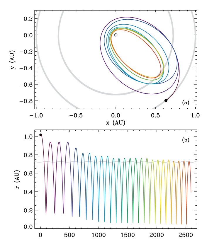
Figure 1: (a) Planned SPP trajectory shown projected in the ecliptic plane, compared with orbits of Venus and the Earth (gray tracks). (b) Heliocentric radial distance of SPP shown versus mission time in days. In both panels, the position of the Earth on July 31, 2018 is indicated with a black circle, and mission time is mapped to curve color.

Figure 1 illustrates the latest version of the proposed SPP baseline mission trajectory. This information was extracted from a SPICE kernel file distributed to the SPP team in September 2014. It assumes a launch date of July 31, 2018, and it extends to September 1, 2025. The kernel data were processed with version N65 of the SPICE toolkit for IDL (Acton, 1996), which was created by the NASA/JPL Navigation and Ancillary Information Facility (NAIF). The Cartesian $(x,y,z)$ positions of SPP, in solar-system barycenter coordinates for epoch J2000.0, were computed and saved at 0.1 day intervals. The mission time $t$ shown in Figure 1(b) is specified in days measured from 0:00 UT on July 31, 2018.

The dynamical properties of 97 Mercury-crossing asteroids were obtained from the NASA/JPL Horizons On-Line Ephemeris System (Giorgini et al., 1996; Giorgini, 2011) in July 2015. The Horizons system was used to convert the tabulated orbital elements into Cartesian $(x,y,z)$ positions, which we saved at 12 hour intervals during the calendar years 2018 to 2026. In order to compare directly with the SPP trajectory data, each asteroid’s coordinates were interpolated to the denser (0.1 day) time grid obtained from the spacecraft SPICE kernel.

The specific asteroids appropriate for this study were selected with the following criteria. First, we included all 63 known asteroids with perihelia less than 0.2 AU. The asteroid that approaches closest to the Sun is 2005 HC₄, with perihelion $q=0.07066$ AU (i.e., 15.2 $R_{\odot}$). There are six others with perihelia less than 0.1 AU. Second, the database was extended to asteroids with perihelia between 0.2 and 0.3 AU. However, out of the 159 known asteroids in this region, many of them are extremely small and dim. The results of Sections 4–5 below show that only the largest asteroids at $q>0.2$ AU are expected to display substantial mass loss. Thus, we selected the brightest 34 of that group, with the criterion that their $V$-band absolute magnitudes $H$ must be $\leq 18.0$. No asteroids were chosen with $q>0.3$ AU because of both their negligible expected mass loss rates and the infrequency of close encounters with SPP once it enters the inner heliosphere. Table 1 gives the final list of 97 asteroids in order of increasing perihelion $q$, and it also lists their names/numbers, eccentricities $e$, and $V$-band magnitudes $H$.

Table 1: Inner heliospheric asteroids tracked in this study, sorted by perihelion.

Number	Name	$q$ [AU]	$e$	$H$ [mag]	$d_{\rm min}$ [AU]	$r_{a}(d_{\rm min})$ [AU]
—	2005 HC4	0.07066	0.96119	20.7	0.10941	0.11916
—	2008 FF5	0.07914	0.96539	23.1	0.28942	0.46209
—	2015 EV	0.08003	0.96100	22.5	0.64377	0.07659
394130	2006 HY51	0.08100	0.96884	17.2	0.32687	0.41537
137924	2000 BD19	0.09199	0.89505	17.2	0.07756	0.10245
374158	2004 UL	0.09283	0.92670	18.8	0.16533	0.22027
394392	2007 EP88	0.09558	0.88584	18.5	0.12213	0.21280
—	2011 KE	0.10013	0.95502	19.8	0.15917	0.39329
—	2008 HW1	0.10171	0.96061	17.4	0.55013	0.25181
—	2015 HG	0.10472	0.95025	21.0	0.35597	0.13877
—	2012 US68	0.10566	0.95776	18.3	0.15636	0.46061
—	2011 XA3	0.10859	0.92597	20.5	0.26899	0.39000
399457	2002 PD43	0.11031	0.95603	19.1	0.41708	0.48005
386454	2008 XM	0.11107	0.90913	20.0	0.13714	0.29387
431760	2008 HE	0.11337	0.94993	18.1	0.21685	0.12394
—	2007 EB26	0.11573	0.78867	19.6	0.01372	0.20750
276033	2002 AJ129	0.11671	0.91488	18.7	0.36247	0.15895
—	2000 LK	0.11788	0.94590	18.4	0.54865	0.26888
425755	2011 CP4	0.11813	0.87039	21.2	0.12991	0.24157
—	1995 CR	0.11931	0.86846	21.7	0.20231	0.23316
—	2007 GT3	0.12088	0.93938	19.7	0.55496	0.12185
—	2004 QX2	0.12498	0.90291	21.7	0.07061	0.69866
—	2011 BT59	0.12859	0.94848	21.0	0.25844	0.14597
289227	2004 XY60	0.13017	0.79669	18.9	0.07934	0.13191
—	2015 KO120	0.13120	0.92577	22.0	0.05460	0.67427
—	2007 PR10	0.13241	0.89262	20.7	0.21100	0.75243
—	2006 TC	0.13561	0.91184	18.8	0.22618	0.23233
—	2013 JA36	0.13750	0.94854	21.0	0.43394	0.58412
—	2008 MG1	0.13886	0.82271	19.9	0.03179	0.90056
—	2013 HK11	0.13901	0.93678	20.7	0.04258	0.15407
3200	Phaethon	0.14004	0.88984	14.6	0.24292	0.26831
—	2013 YC	0.14104	0.94347	21.3	0.63135	0.15442
—	2010 JG87	0.14432	0.94773	19.1	0.48764	0.40593
—	2015 KP157	0.14820	0.91027	19.2	0.17604	0.57849
—	2015 DU180	0.15228	0.92097	20.8	0.24979	0.18051
—	2012 UA34	0.15597	0.80155	19.5	0.05960	0.35570
—	2005 EL70	0.15893	0.94022	24.0	0.10759	0.36308
155140	2005 UD	0.16287	0.87224	17.3	0.06729	0.17065
364136	2006 CJ	0.16580	0.75492	20.2	0.02326	0.21205
105140	2000 NL10	0.16727	0.81704	15.8	0.23609	0.44102
—	2011 WN15	0.17285	0.85793	19.6	0.17488	0.17701
—	2013 WM	0.17466	0.91598	23.8	0.53346	0.25236
302169	2001 TD45	0.17733	0.77742	19.9	0.12274	0.59688
—	2005 RV24	0.17805	0.88177	20.6	0.20295	0.75445
—	2008 EY68	0.17888	0.75994	22.0	0.12325	0.17417
141851	2002 PM6	0.17955	0.85012	17.7	0.08396	0.58174
267223	2001 DQ8	0.18138	0.90150	18.0	0.06021	0.18495
—	2013 AJ91	0.18187	0.92818	19.3	0.18173	0.32416
259221	2003 BA21	0.18350	0.83321	19.1	0.06899	0.23841
—	2011 YX62	0.18409	0.92823	23.0	0.26575	0.46486
1566	Icarus	0.18652	0.82696	16.9	0.21870	0.29748
89958	2002 LY45	0.18675	0.88625	17.0	0.14820	0.22125
—	2009 HU58	0.18686	0.90955	19.1	0.11882	0.34948
5786	Talos	0.18727	0.82684	17.1	0.32613	0.78989
—	2003 UW29	0.18899	0.83840	20.7	0.06178	0.35127

Table 1: (continued)   Inner heliospheric asteroids tracked in this study, sorted by perihelion.

Number	Name	$q$ [AU]	$e$	$H$ [mag]	$d_{\rm min}$ [AU]	$r_{a}(d_{\rm min})$ [AU]
387505	1998 KN3	0.19537	0.87328	18.4	0.18166	0.20196
—	2007 MK6	0.19586	0.81879	19.9	0.29098	0.37447
—	2015 KJ122	0.19613	0.75026	22.0	0.06455	0.50995
—	2015 DZ53	0.19620	0.87013	20.8	0.40446	0.20443
—	2010 VA12	0.19875	0.84334	19.5	0.07376	0.22421
—	1996 BT	0.19978	0.83500	23.0	0.10126	0.37595
153201	2000 WO107	0.19985	0.78072	19.3	0.19124	0.35397
139289	2001 KR1	0.19996	0.84123	17.6	0.02376	0.47075
66391	1999 KW4	0.20010	0.68846	16.5	0.12587	0.20703
141079	2001 XS30	0.20015	0.82815	17.7	0.03979	0.20640
143637	2003 LP6	0.20341	0.88352	16.3	0.31278	0.51759
329915	2005 MB	0.20411	0.79284	17.1	0.33105	0.54317
438116	2005 NX44	0.20495	0.90745	17.3	0.35076	0.81328
369296	2009 SU19	0.20935	0.89942	17.9	0.06908	0.26797
184990	2006 KE89	0.21144	0.79925	16.4	0.14092	0.52566
—	2004 LG	0.21250	0.89714	18.0	0.39704	0.38711
—	2005 GL9	0.22226	0.89620	17.1	0.03307	0.22339
137052	Tjelvar	0.23768	0.80955	16.9	0.08579	0.24021
225416	1999 YC	0.24099	0.83050	17.2	0.29616	0.31271
—	2000 SG8	0.24508	0.90066	17.5	0.59763	0.75514
242643	2005 NZ6	0.24872	0.86443	17.4	0.08031	0.81175
136874	1998 FH74	0.25390	0.88462	15.7	0.29403	0.29322
40267	1999 GJ4	0.25669	0.80825	15.4	0.31560	0.25078
—	2011 WS2	0.25890	0.74356	17.2	0.16082	0.32279
—	2007 VL243	0.26200	0.72856	17.8	0.04606	0.46376
331471	1984 QY1	0.26348	0.89453	15.4	0.28198	0.34163
—	2006 OS9	0.26379	0.90377	17.8	0.21360	0.35270
369452	2010 LG14	0.26898	0.74267	17.9	0.32184	0.36409
190119	2004 VA64	0.27010	0.89042	17.1	0.41024	0.37468
351370	2005 EY	0.27510	0.89066	17.2	0.12769	0.27657
164201	2004 EC	0.28058	0.85954	15.7	0.12414	0.28329
385402	2002 WZ2	0.28476	0.88432	17.0	0.47899	0.34397
397237	2006 KZ112	0.28545	0.88694	16.7	0.75831	0.66348
253106	2002 UR3	0.28549	0.79295	16.4	0.52059	0.66113
364877	2008 EM9	0.29101	0.85153	17.3	0.08666	0.34927
—	2014 MR26	0.29387	0.76593	17.8	0.12435	0.66948
231937	2001 FO32	0.29523	0.82644	17.7	0.20666	0.32020
99907	1989 VA	0.29525	0.59468	17.9	0.24233	0.31057
170502	2003 WM7	0.29648	0.88027	17.2	0.20954	0.77615
—	2010 KY127	0.29686	0.88116	17.0	0.51914	0.36652
162269	1999 VO6	0.29734	0.73809	17.0	0.26966	0.34300
141525	2002 FV5	0.29916	0.72475	17.9	0.21795	0.33586

A set of 97 timelines containing the relative positions of SPP, the asteroid, and the Sun were produced from the ephemeris data over the 2018–2025 mission period. The three mutual distances $d$ (between SPP and asteroid), $r_{a}$ (between Sun and asteroid), and $r_{p}$ (between Sun and SPP) are used for various purposes in the models described below. Other useful quantities include the solar elongation angle $\varepsilon$ (i.e., the angle centered on SPP between vectors pointing to the Sun and to the asteroid) and the scattering phase angle $\alpha$ (i.e., the angle centered on the asteroid between vectors pointing to the Sun and to the observer on SPP). Both angles can be computed from the three distances,

$$\cos\varepsilon\,=\,\frac{r_{p}^{2}+d^{2}-r_{a}^{2}}{2r_{p}d}\,\,\,,\,\,\,\,\,\,\,\,\,\cos\alpha\,=\,\frac{r_{a}^{2}+d^{2}-r_{p}^{2}}{2r_{a}d}\,\,\,.$$ (1)

Table 1 lists $d_{\rm min}$, the distance of closest approach for each asteroid to SPP, and the value of $r_{a}$ at that time. The asteroid with the smallest value of $d_{\rm min}$ is 2007 EB₂₆, with a minimum separation of only 0.0137 AU (i.e., 2.95 $R_{\odot}$), which should occur at $t=779.5$ days. There are 24 asteroids in the list that come closer than 0.1 AU to SPP.

Figure 2 shows the spread of minimum distance $d_{\rm min}$ versus each asteroid’s perihelion distance $q$. There is no overall correlation between these quantities, but there does appear to be a slight preponderance (see dashed line) for asteroids with the largest $q$ values to avoid close approaches with SPP. This is likely to be a statistical trend associated with the fact that asteroids with wider orbits naturally spend less time in SPP’s neighborhood close to the Sun.

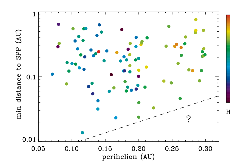
Figure 2: Minimum distances $d_{\rm min}$ between SPP and each asteroid, found by comparing ephemerides between July 31, 2018 and September 1, 2025. The symbol colors map to asteroid absolute magnitude $H$.

It should be emphasized that the accurate prediction of a close approach between SPP and any specific asteroid depends on the validity of the planned trajectory and launch date of July 31, 2018. Spacecraft launches are frequently delayed, but SPP does have firm requirements to “meet” the desired gravitational assists with Venus. Thus, it is possible that even a delayed launch could result in an eventual synchronization with the trajectory assumed here. In any case, some results of this paper may be better interpreted as one possible sample from a quasi-random distribution of possible SPP orbits. Additional statistical conclusions are discussed in Section 6.

As an example of an interesting encounter, Figure 3(a) shows the mutual trajectories for SPP and asteroid 137924 (2000 BD₁₉). This example is only the 19th closest approach out of the full list of 97 asteroids, but it is notable for occurring very near the asteroid’s own perihelion. That fact leads to it having a bright $V$ magnitude and unusually high predicted values for its mass loss rate and coma size (see below). Figure 3(b) also shows that, for the case of asteroid 137924, multiple close encounters with SPP tend to occur near successive perihelion passes.

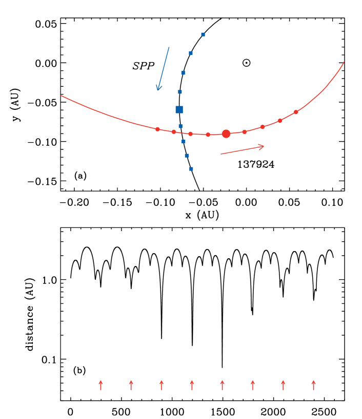
Figure 3: (a) Trajectories for the closest encounter between SPP (black curve) and asteroid 137924 (red curve). Large symbols show positions at minimum distance, at mission time 1493.68 days. Smaller symbols show the positions along a sequence of 7.2 hr intervals before and after the time of minimum distance. (b) Relative distance between SPP and asteroid 137924 versus mission time in days. Red arrows show the times of the asteroid’s perihelia.

3 Asteroid Physical Properties

In the analysis performed below, each asteroid is assumed to be spherical in shape, with a diameter $D$ given by a standard conversion from its visible-light absolute magnitude $H$,

$$D\,=\,\left(1348\,p^{-1/2}\,10^{-H/5}\right)\,\,\,\,\,\mbox{km}\,\,,$$ (2)

(e.g., Bowell et al., 1989), where we take $p=0.1$ as a representative value of the geometric albedo for small asteroids in the inner heliosphere (see also Muinonen et al., 1995; Morbidelli et al., 2002). For the 97 asteroids listed in Table 1, the median derived value of $D$ is 0.890 km, and the minimum and maximum values are 0.0675 km (2005 EL₇₀) and 5.12 km (3200 Phaethon), respectively. Their angular sizes, as seen by SPP, are typically in the range between 0.001^′′ and 0.03^′′, with the largest value of 0.075^′′ found for the closest approach of asteroid 2001 KR₁. These values are much smaller than the spatial resolution of the WISPR telescopes. However, we anticipate that many asteroids will emit bright dust clouds that extend to distances several orders of magnitude larger than their respective diameters (see Section 5).

The apparent magnitude of an asteroid in the Johnson–Cousins $V$ band (dominated by wavelengths between 500 and 600 nm) is given by

$$m_{V}\,=\,H+5\log_{10}(r_{a}d)-2.5\log_{10}\Phi(\alpha)$$ (3)

where $r_{a}$ and $d$ are given in units of AU. $\Phi(\alpha)$ is the phase function for the scattering of sunlight, which is largest at opposition ($\alpha=0$) and decreases monotonically for larger scattering angles. The standard phase function defined by Bowell et al. (1989) was used with a slope parameter $G=0.15$ appropriate for inner heliospheric asteroids (see also Lagerkvist and Magnusson, 1990). Apparent magnitudes were converted into $V$-band energy fluxes at $\lambda\approx 500$ nm, with

$$F\,=\,3.67\times 10^{-23}\,(10^{-0.4m_{V}})\,\,\,\,\mbox{W m${}^{-2}$ Hz${}^{-1}$}$$ (4)

using the normalization factor specified by Wamsteker (1981). Figure 4(a) shows the distribution of $m_{V}$ versus minimum distance $d_{\rm min}$. The brightest one is asteroid 141079, with $m_{V}=8.95$, but there is nothing unusual about its intrinsic properties. Finding a small value of $m_{V}$ depends on the chance of finding small values for $d$, $r_{a}$, and $\alpha$, all occurring at roughly the same time.

The observability of a given asteroid depends on both its intrinsic brightness and its relative contrast with the sky background. Jewitt et al. (2013) observed 3200 Phaethon and its tail with the Sun Earth Connection Coronal and Heliospheric Investigation (SECCHI) package on STEREO (Howard et al., 2008; Eyles et al., 2009), and they noted how measurements were limited by the presence of extended sky emission. The WISPR instrument on SPP will be closer to its asteroid targets than was SECCHI, and it will have comparable sensitivity despite its smaller size. Thus, in this paper we apply several of the lessons learned from SECCHI to future measurements with WISPR.

Visible-light sky emission in the inner heliosphere is dominated by a combination of zodiacal light (the dust-scattered F corona) and Thomson-scattered electron emission (the K corona). A relatively simple analytic expression for the total specific intensity $B_{Z}(\varepsilon,r_{p})$ of the two components was found to reproduce a range of observations and model predictions. For a standard observer at $r_{p}=1$ AU, the angular dependence is given by

$$\frac{B_{Z}(\varepsilon,\mbox{1 AU})}{B_{\odot}}\,=\,\frac{4\times 10^{-25}}{\varepsilon^{8}}+\frac{6.3\times 10^{-14}}{[\sin(0.63\varepsilon)]^{2.22}}$$ (5)

where the elongation angle $\varepsilon$ is specified in radians and the mean solar-disk brightness is $B_{\odot}=2.96\times 10^{-8}$ W m^-2 sr^-1 Hz^-1 in the $V$ band (Allen, 1973). Equation (5) matches collected observations in the ecliptic plane (Leinert, 1975; Munro & Jackson, 1977; Kwon et al., 2004; Mann et al., 2004) to within about a factor of two. Observers closer to the Sun are expected to see higher intensities (e.g., van Dijk et al., 1988), and we use

$$B_{Z}(\varepsilon,r_{p})\,=\,B_{Z}(\varepsilon,\mbox{1 AU})\,\left(\frac{\mbox{1 AU}}{r_{p}}\right)^{2.5}$$ (6)

where the exponent 2.5 was estimated from the modeled inner heliospheric intensities in Figure 7 of Vourlidas et al. (2015).

The goal is to compare the above sky brightness with the flux from an asteroid, but the latter is essentially a tiny point-source with an angular size much smaller than a WISPR detector pixel. The asteroid’s flux $F$ must be compared with a corresponding sky flux $F_{Z}$ that fills the pixel. The zodiacal light intensity $B_{Z}$ is thus converted into flux by multiplying it by the solid angle subtended by a pixel, with

$$F_{Z}\,=\,\Omega\,B_{Z}(\varepsilon,r_{p})\,\,.$$ (7)

Vourlidas et al. (2015) specified pixel sizes of 1.2^′ and 1.7^′ for the inner and outer fields of view, and we used the average of the two as a representative value. Thus, a square patch of the sky subtending $1.45^{\prime}=4.22\times 10^{-4}$ radians on a side occupies a solid angle $\Omega=1.78\times 10^{-7}$ sr.

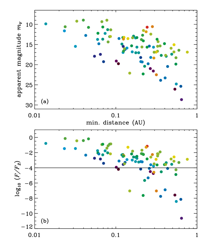
Figure 4: (a) Apparent magnitudes, at times of closest approach with SPP, plotted versus minimum distance between each asteroid and SPP. (b) $V$-band asteroid flux $F$ divided by the estimated zodiacal light flux $F_{Z}$ measured in a single WISPR pixel. The horizontal line shows an approximate observable threshold of $10^{-4}$ times the background. In both panels, symbol colors correspond to $H$ with the same scaling as in Figure 2.

Figure 4(b) shows the ratio $F/F_{Z}$ as a function of $d_{\rm min}$. Differences with panel (a) are mainly due to the fact that different asteroids are viewed with different elongation angles, so the sky brightness varies. The highest-contrast asteroid is 2001 KR₁, with $F/F_{Z}=0.72$. Ideally, one would consider a “good” observation to be one with $F\gg F_{Z}$, but experience with SECCHI has shown that much weaker signals can be extracted from strong backgrounds. DeForest et al. (2011) used sophisticated processing techniques to resolve features with fluxes as low as $(F/F_{Z})\approx 10^{-4}$. That level is indicated with a horizontal line in Figure 4(b), and we note that 76 out of 97 asteroids fall above that level. WISPR will clearly have multiple opportunities to observe asteroids in the inner heliosphere.

It is noteworthy that the list of five brightest (i.e., lowest $m_{V}$) asteroids and the list of five highest flux contrast (largest $F/F_{Z}$) asteroids share three members: 141079, 2005 GL₉, and 2007 EB₂₆. Note that asteroid 137924, whose orbit is shown in Figure 3, is the second brightest ($m_{V}=8.98$) at closest approach, but due to a low elongation angle it is only the 14th highest flux contrast ($F/F_{Z}=0.038$). The largest active asteroid, 3200 Phaethon, has its lowest value of $m_{V}=10.53$ at $t=1384.6$, about six days prior to the time it reaches its minimum distance $d_{\rm min}$ to SPP. However, because of varying elongation angles, Phaethon’s time of maximum flux contrast (at $F/F_{Z}=0.13$) occurs at its previous perihelion passage 17 months earlier ($t=880.3$). This tells us that the “snapshots” of the 97 closest-approach events, illustrated by filled circles in Figures 2 and 4, may not always be the most reliable guide to identifying when interesting things are occurring.

4 Asteroid Mass Loss due to Erosion

In a similar manner to comets, it is believed that active asteroids lose mass when they orbit sufficiently close to the Sun. The ejected gas and dust expands to fill coma-like or tail-like atmospheres that may be observed at large distances from the nucleus. One can use the language of sublimation to discuss the erosion of solid material from the asteroid surface. Some active asteroids (e.g., 133P/Elst-Pizzaro in the main asteroid belt; see Hsieh et al., 2004) are probably similar to comets in that they emit gaseous mass mostly in the form of volatile ices (H₂O, CO, CO₂). However, the near-Sun active asteroids (e.g., Phaethon) have likely already lost most of these easily sublimated compounds. The heavier silicate and hydrocarbon molecules that presumably dominate the outer regolith layers of these asteroids have a substantially higher latent heat than volatile comet ices. This section applies the long history of sublimation energy-balance models for comets (e.g, Weigert, 1959; Delsemme and Miller, 1971; Whipple and Huebner, 1976; Weissman, 1980; Prialnik et al., 2004) to the case of near-Sun active asteroids.

Before proceeding with such modeling, it is important to note that the loss of both silicate-rich gas and dust from rocky objects (heated to $T\approx 1000$ K) has not been studied as extensively as the standard cometary scenario of sublimating ice molecules that drag along the larger dust grains. However, the idea of a simultaneous ejection of multiple phases of the same type of material has been studied for comets. Water ice and other volatile compounds appear to be ejected in both the gas phase and in the form of “snow” particles with sizes ranging from microns to meters (e.g., Delsemme and Miller, 1971; Kelley et al., 2013, 2015; Protopapa et al., 2014).

In addition to the analogy with comet ice loss, there are three other comparable situations that appear to have some resemblance and relevance to the case of active asteroids:

1. Meteors entering a planetary atmosphere undergo rapid deceleration and thermal ablation (e.g., Baldwin and Sheaffer, 1974). Although the source of heating for meteors is different (atmospheric drag versus solar radiation), the mass loss is often treated by replacing the latent heat of sublimation with a comparable heat of ablation (Chyba et al., 1993). The size distribution of resulting fragments appears to be quite broad, from nanometer-scale “smoke” to micron-scale dust to macroscopic meteoroids (Borovička and Charvát, 2009; Malhotra and Mathews, 2011).

2. Sungrazing comets have perihelia within a few solar radii of the Sun’s surface (Marsden, 2005), and observations of their evolution upon close approach provide valuable information about the composition and thermal properties of primordial bodies in the solar system. Sekanina (2003) was able to model the light curves of a number of sungrazing comets by assuming a continuous distribution of silicate erosion products (i.e., from large fragments to individual sublimated molecules). These comets have also been observed to emit metallic—i.e., alkali, sulfide-rich, and iron-group—material as well (Preston, 1967; Slaughter, 1969; Zolensky et al., 2006; Ciaravella et al., 2010),

3. We now know that a large number of extrasolar planets orbit within just a few stellar radii of their host stars (Winn and Fabrycky, 2015). Some observations suggest that small, rocky planets of this kind are slowly disintegrating via the ejection of large amounts of dust (e.g., Mura et al., 2011; Rappaport et al., 2012; van Lieshout et al., 2014; Sanchis-Ojeda et al., 2015). Possible formation channels for the dust include condensation from sublimated gas, direct ejection via volcanism, or comet-like entrainment of grains along with escaping gas molecules.

Thus, there appear to be multiple ways that silicate-rich gas can be removed from the surfaces of solid objects near the Sun, together with larger dust grains, when they experience strong solar irradiation. It should also be mentioned that the minerals left on the surfaces of these bodies may be irradiated sufficiently to induce various types of chemical and tensile metamorphosis (Scott et al., 1989; Scheeres, 2005; Kasuga et al., 2006; Gundlach and Blum, 2016).

The thermal energy balance at the surface of a solid body can be solved to compute the mass loss rate $\dot{M}$ and equilibrium temperature $T$ of molecules leaving the surface. Ignoring heat conduction, the short-wave radiative energy gained must be balanced by losses due to long-wave radiation and sublimation, with

$$\frac{(1-A)S_{\odot}}{r_{a}^{2}}\cos\theta\,=\,\eta\sigma_{\rm B}T^{4}\,+\,m_{u}LZ$$ (8)

where $A$ is the asteroid’s Bond albedo, $S_{\odot}$ is the solar constant, $\theta$ is the angle between rays from the Sun and the asteroid surface normal, $\sigma_{\rm B}$ is the Stefan-Boltzmann constant, $\eta$ is the emissivity of the asteroid surface, $m_{u}$ is the atomic mass unit, $L$ is the latent heat of sublimation of the escaping gas, specified here as an energy per mole, and $Z$ is the surface sublimation rate (particles lost per unit area per unit time). For simplicity, some of these quantities are fixed at constant values of $A=0.1$, $\eta=1$, and $S_{\odot}=1360$ W m^-2.

Although the resulting rate of mass loss is sensitive to details of the Sun–asteroid geometry, it is possible to discuss the behavior in two limiting cases for $\cos\theta$ (see Jewitt et al., 2011, 2015). A rapidly rotating asteroid will redistribute the incoming radiative energy from its Sun-facing side over the majority of its emitting surface. In that case, a mean value of $\cos\theta=1/4$ accounts for this efficient redistribution. On the other hand, a slowly rotating (or non-rotating) asteroid will receive most of its energy at nearly sub-solar surface locations, and will emit sublimated gas only from the illuminated parts. Thus, one can assume $\cos\theta=1$ at those locations. In these two cases the emitting surface area $A$ of the asteroid also differs. In the fast-rotating limit, nearly all points on the asteroid receive some heat, so $A\approx\pi D^{2}$ (the full surface area). In the slow-rotating limit, the area is given roughly by the front-side cross section, $A\approx\pi D^{2}/4$. This area is needed to compute the full mass loss rate

$$\dot{M}\,=\,Z\mu m_{u}A\,\,,$$ (9)

where $\mu$ is the mean molar mass of the sublimating molecules. The quantity $Z\mu m_{u}$ is sometimes called the mass erosivity $\dot{\epsilon}$ (mass lost per unit time per unit area).

Equation (8) has two undetermined parameters: $T$ and $Z$. These can be found by using the Clausius–Clapeyron relation, which specifies the vapor pressure $P_{v}$ at the surface of a sublimating body,

$$P_{v}\,=\,P_{\infty}\,\exp\left(-\frac{m_{u}L}{k_{\rm B}T}\right)$$ (10)

where $P_{\infty}$ is the vapor pressure in the high-temperature limit and $k_{\rm B}$ is Boltzmann’s constant. The latent heat is assumed to be a constant, independent of temperature. Assuming a Maxwellian distribution of escaping molecules, the mean sublimation rate at the surface is given by the Hertz–Knudsen equation,

$$Z\,=\,\frac{\gamma\,P_{v}}{\sqrt{2\pi\mu m_{u}k_{\rm B}T}}$$ (11)

where $\gamma$ is a dimensionless efficiency that takes account of a range of kinetic effects (see, e.g., van Lieshout et al., 2014).

Table 2: Sublimation properties of cometary and asteroidal substances.

Substance	$\mu$	$\rho$	$L$	$\ln P_{\infty}$	$\gamma$	Refs
	[g/mol]	[g/cm3]	[kJ/mol]	[ln Pa]
Carbon dioxide (CO2)	44.00	1.56	26.34	27.84	1.0	1
Water ice (H2O)	18.00	1.00	48.06	28.90	1.0	2
Sodium (Na)	23.00	0.97	105.80	22.53	1.0	3
Carbonaceous chondrite	39.85	2.80	320.67	24.48	1.0	4
Iron (Fe)	55.85	7.87	402.03	26.90	1.0	5
Silicon monoxide (SiO)	44.09	2.13	411.72	30.20	0.04	5
Fayalite (Fe2SiO4)	203.77	4.39	501.99	35.40	0.1	5
Enstatite (MgSiO3)	100.39	3.20	572.92	35.80	0.1	5
Forsterite (Mg2SiO4)	140.69	3.27	542.99	31.80	0.1	5
Quartz (SiO2)	60.08	2.60	577.38	30.80	1.0	5
Corundum (Al2O3)	101.96	4.00	643.24	37.00	0.1	5
Silicon carbide (SiC)	40.10	3.22	652.36	35.50	0.1	5
Graphite (C)	12.01	2.16	778.60	34.40	0.1	5

References: 1.  Fanale and Salvail (1987), 2.  Fanale and Salvail (1984), 3.  Huebner (1970), 4.  Baldwin and Sheaffer (1974), 5.  van Lieshout et al. (2014).

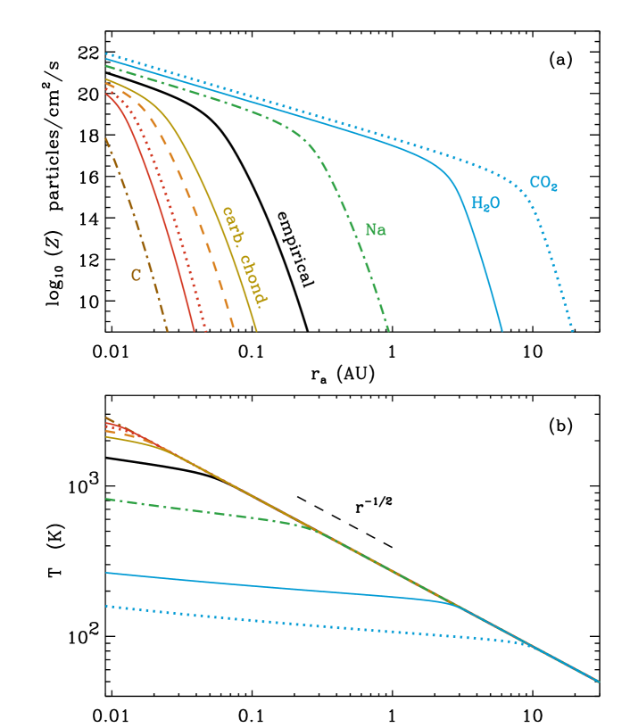
Figure 5: Dependence on asteroid heliocentric distance $r_{a}$ of: (a) surface sublimation rates $Z$ and (b) energy-balance temperatures $T$, plotted for a subset of the substances listed in Table 2. Unlabeled curves correspond to atomic iron (orange dashed curve), crystalline enstatite (red dotted curve), and corundum (red solid curve). See text for discussion of the empirical model (black solid curve).

Table 2 lists many of the above properties for substances believed to exist on comets and asteroids, listed in order of increasing latent heat. Figure 5(a) shows numerical solutions for $Z$ as a function of heliocentric distance $r_{a}$, for a subset of the substances listed in Table 2. In most cases there is an inverse monotonic relationship between $L$ and $Z$ at any given distance. Close to the Sun, the sublimation term dominates the right-hand side of Equation (8), and thus $Z\propto r_{a}^{-2}$. At larger distances, $Z$ drops off exponentially when the radiative emission term begins to dominate. The fast-rotating limit was used to compute $\cos\theta$ and $A$ because observations (e.g., Campins et al., 2009) suggest inner heliospheric asteroids experience significantly more surface redistribution of thermal energy than predicted by non-rotating models.

Figure 5(b) shows the associated energy-balance solutions for the surface temperature $T$. For the most volatile substances, $T$ is relatively flat near the Sun because the incoming solar flux drives the sublimation phase change and does not heat up the asteroid. In that case, the quantity $1/T$ varies approximately as $(c_{1}+c_{2}\ln r_{a})$ for appropriate constants $c_{1}$ and $c_{2}$. Farther from the Sun, however, $T\propto r^{-1/2}$ in radiative equilibrium.

Because we do not yet know the detailed surface composition of active asteroids, it is not clear how to specify the latent heat and other properties a priori. Sekanina (2003) modeled the light curves of sungrazing comets by treating the latent heat $L$ and mean molecular mass $\mu$ as constrained free parameters. The result of that process was a range of latent heats (120 to 360 kJ mol^-1) and molecular masses (200 to 800 g mol^-1), with unique pairs of values that successfully predict the light curve properties of each comet. Figure 6 compares laboratory values of $L$ and $\mu$ for the substances listed in Table 2 with those derived empirically by Sekanina (2003). Shown for comparison are data from other listings of volatile ices (Prialnik et al., 2004) and solid-phase elements (Huebner, 1970). In this two-dimensional plane, there is no real overlap between the laboratory values and those derived by Sekanina (2003). However, it is important to note that the sublimation rate $Z$ is driven mainly by the value of $L$ and only very weakly by $\mu$ (i.e., $Z\propto\mu^{-1/2}$). Thus, the overlap that is seen in just the $L$ values may point to the existence of a heterogeneous mixture of substances with a range of sizes and latent heats (e.g., hydrated silicates mixed with organic hydrocarbons) that could be released from surfaces exposed to the near-Sun environment.

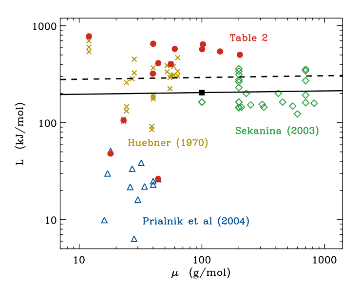
Figure 6: Comparison of laboratory measurements of the sublimation properties of solid substances (red filled circles from Table 2; gold crosses from Huebner 1970; blue triangles from Prialnik et al. 2004) with empirical determinations from sungrazing comet light curves (green diamonds from Tables 1 and 3 of Sekanina 2003). Contours that reproduce the measured mass loss of Phaethon are shown in black (solid: fast-rotating limit, dashed: slow-rotating limit).

In a similar vein as the empirical study of Sekanina (2003), it is possible to use the Jewitt et al. (2013) measurement of Phaethon’s mass loss ($\dot{M}\approx 3$ kg s^-1 at perihelion) to provide an observation-based estimate of $L$ and $\mu$. However, the measured value of $\dot{M}$ from Phaethon was a dust mass loss rate, whereas the quantity computed in Equation (9) corresponds to the gas/molecular component of the outflow. As stated above, there is still no firmly accepted understanding of how active asteroids produce and eject dust grains. The gas and dust components may be intimately connected to one another (via, e.g., re-condensation of sublimated molecules) or they may originate from completely different regions on the surface (see Jewitt et al., 2015). However, we can note that many comets are inferred to have dust-to-gas mass ratios ${\cal M}$ centered around unity (e.g., A’Hearn et al., 1995; Sanzovo et al., 1996; Kolokolova et al., 2007). Thus, we make a trial assumption of ${\cal M}=1$, which allows us to take $\dot{M}$ to be equal to the dust mass loss rate. The assumed value of ${\cal M}$ is likely to be an important source of uncertainty for the model results given below. The sensitivity of these results to changes in ${\cal M}$ is explored further below as well.

An empirical model of the sublimation of material with arbitrary $L$ and $\mu$ requires specification of the other sublimation properties of the material. We follow Huebner (1970) and Sekanina (2003) by defining

$$P_{\infty}\,=\,P_{0}\,\exp\left(\frac{m_{u}L}{k_{\rm B}T_{0}}\right)$$ (12)

with a fiducial value of $P_{0}=0.398$ GPa. The result of computing $T_{0}$ for the 13 actual substances listed in Table 2 is a mean value (after excluding CO₂ and H₂O) of 5300 K, which is used in the models below. Since the assumed heterogeneous mixture of substances may contain both dusty ices ($\gamma\approx 1$) and silicates ($\gamma\approx 0.1$) we assume a mean value of $\gamma=0.3$.

A comprehensive search of the two-dimensional space shown in Figure 6 was undertaken for a Phaethon-like asteroid at perihelion, with $r_{a}=0.14004$ AU and $D=5.12$ km. Values of $L$ and $\mu$ that yielded $\dot{M}=3$ kg s^-1 are shown by the black curves in Figure 6; one computed for the fast-rotating limit and one for the slow-rotating limit. For simplicity, we choose one point along the fast-rotating locus of solutions for use in the models presented below: $L=204$ kJ mol^-1 and $\mu=100$ g mol^-1 (see the black filled square in Figure 6). This value of $L$ falls comfortably within the empirically determined range found by Sekanina (2003) for sungrazing comets. Also, our solutions are close to the value of 320 kJ mol^-1 listed in Table 2 for carbonaceous chondrites. It should be noted that the value of $L$ for chondritic material is not really known so precisely. Both Baldwin and Sheaffer (1974) and Chyba et al. (1993) reported approximate values for the heat of ablation of chondrite meteors spanning values between 200 and 350 kJ mol^-1. To repeat, we believe this empirical solution may point to the existence of a mixture of multiple solid species that, taken in bulk, sublimate at a similar rate as a single compound with representative values of $L$ and $\mu$.

Figure 7 shows computed mass loss rates versus $r_{a}$ for this paper’s collection of 97 closest-approach events with SPP, and we use the empirical solution described above: $L=204$ kJ mol^-1 and $\mu=100$ g mol^-1 in the fast-rotating limit. When these parameters are held fixed, it is clear that $r_{a}$ is the parameter most important for determining $\dot{M}$, with the asteroid diameter $D$ providing a much more limited variation. The red filled circle indicates the position of asteroid Phaethon at its closest approach with SPP, and the red X symbol shows Phaethon at its perihelion. At the time of closest approach with SPP, Phaethon’s mass loss rate is predicted to be almost a million times lower than when it reaches perihelion. This again provides a warning that the times of closest approach may not be the most auspicious observation times. Observations of Phaethon and several other asteroids taken at larger distances ($r_{a}=1.4$–2.6 AU; see Jewitt, 2013) showed no discernible mass loss. The approximate upper limits on $\dot{M}$ shown in Figure 7 are many orders of magnitude larger than what our model would predict at those distances.

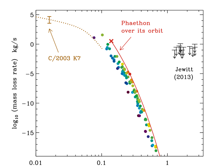
Figure 7: Gas mass loss rates $\dot{M}$ for asteroids at their times of closest approach with SPP (symbols, with colors corresponding to $H$ with same scaling as in Figure 2) and for asteroid 3200 Phaethon at various points along its orbit (red solid curve) and at perihelion (red X symbol). A similar model for comet C/2003 K7 (brown dotted curve) is compared to the measured range of dust $\dot{M}$ values from Ciaravella et al. (2010) (brown strut). Non-detection upper limits from Keck observations of active asteroids far from perihelion (Jewitt, 2013) are shown with black arrows.

Another comparison between observed dust mass loss and the model described above is shown in Figure 7. Ciaravella et al. (2010) observed silicon and carbon ultraviolet emission from sungrazing comet C/2003 K7 when it was at a distance of $r_{a}=0.016$ AU. They deduced a range of dust mass loss rates assuming the silicon comes from the dissociation of molecules like olivine or forsterite. Ciaravella et al. (2010) also inferred a diameter for the nucleus of about 0.06–0.12 km. Using a central value of $D=0.1$ km and the fast-rotating model above with $L=204$ kJ mol^-1, we found values of $\dot{M}$ for the gas that fall within the uncertainty limits of the Ciaravella et al. (2010) dust mass loss rate.

The agreement between the above model and the Ciaravella et al. (2010) observation represents additional support for ${\cal M}\approx 1$ for inner heliospheric mixtures of dust and gas in the vicinity of sublimating bodies. However, if we had chosen other values of ${\cal M}$, it would have only required a small change in the latent heat to reproduce the Jewitt et al. (2013) mass loss rate. Specifically, the standard value of $L=204$ kJ mol^-1 (which was optimized for ${\cal M}=1$) needs to be decreased only to 172 kJ mol^-1 for ${\cal M}=0.01$, or increased to 237 kJ mol^-1 for ${\cal M}=100$. These changes in $L$ have been incorporated into an approximate fitting formula for the sublimation rate $Z$ as a function of both heliocentric distance and the dust-to-gas mass ratio:

$$Z_{\rm fit}(r_{a},{\cal M})\,=\,Z_{0}\,{\cal M}^{-0.0427}\,r_{a}^{-2.25}\,\left[1+(r_{a}/\sigma)^{3}\right]^{-6}\,\,,$$ (13)

where $r_{a}$ is expressed in AU, $Z_{0}=2.545\times 10^{16}$ particles cm^-2 s^-1, and $\sigma=0.0787{\cal M}^{-0.0661}$. This fitting formula is used below in order to vary ${\cal M}$ as a free parameter while retaining the empirical calibration to Phaethon’s dust mass loss rate.

5 Coma and Tail Formation

The goal of this section is to estimate a representative length scale for the dust-filled coma or tail surrounding an active asteroid in the inner heliosphere. This length scale is defined specifically as the largest distance from the asteroid at which WISPR on SPP is expected to see a dust-scattered enhancement over the sky background. As above, we continue to use the observations of Phaethon at its perihelion (Jewitt et al., 2013) to help constrain some of the unknown parameters of the model.

5.1 Spherically Symmetric Model

Huebner (1970) and Delsemme and Miller (1971) computed the maximal radial distance traversed by dust grains that are ejected from a comet’s surface. Newly freed grains become exposed immediately to sunlight and begin to sublimate in the same manner as the parent asteroid. A spherical dust grain with radius $a$ should have a finite lifetime $\tau$ given by

$$\tau\,=\,\frac{\rho a}{\mu m_{u}Z}\,\,\,,$$ (14)

where $\rho$ is the mean mass density of escaping material. In the models below, we assume a representative value $\rho=3$ g cm^-3. A dust grain that drifts away from the parent body with velocity $v_{\rm dust}$ will thus traverse a radial distance of order $R\approx v_{\rm dust}\tau$ before it sublimates away completely. However, Jewitt et al. (2013) speculated that the observed radial distance of coma-like emission is probably going to be smaller than $R$, because instrumental effects (i.e., a high sky background and low photon counting statistics) can obscure the faint outer parts of the dust cloud. Thus, we need to estimate the visible-light brightness of a dust coma (as a function of impact-parameter distance $b$ away from the asteroid) and compare it to the sky background flux $F_{Z}$ defined in Section 3.

In lieu of a full three-dimensional model of the dynamics of dust grains leaving the asteroid, an approximate spatial distribution can be computed using the model of Haser (1957). Making use of mass flux conservation in spherical symmetry, with a sink term to account for grain loss via sublimation, results in a time-steady solution for the dust number density,

$$n_{d}(r)\,=\,n_{d0}\left(\frac{R_{a}}{r}\right)^{2}\exp\left[-\left(\frac{r-R_{a}}{v_{\rm dust}\tau}\right)\right]\,\,,$$ (15)

where $R_{a}$ is the asteroid radius and $r$ is the asteroid-centric radial distance at which $n_{d}$ is measured. The value of $n_{d0}$ at the asteroid surface can be estimated if we know the dust-to-gas mass ratio ${\cal M}$ and the number density of gas molecules $n_{g0}$ at the surface,

$$n_{d0}\,=\,\frac{(\mu m_{u})\,n_{g0}}{m_{d}}\,\,{\cal M}$$ (16)

and $m_{d}$, the mass of an individual dust grain, can be computed straightforwardly given its mean density $\rho$, radius $a$, and the assumption it is roughly spherical in shape. The Maxwellian gas mass loss theory (Equation 11) also specifies

$$n_{g0}\,=\,4Z\,/\,\bar{v}$$ (17)

where the mean speed of gas molecules is given by

$$\bar{v}\,=\,\sqrt{\frac{8k_{\rm B}T}{\pi\mu m_{u}}}$$ (18)

(e.g., Delsemme and Miller, 1971).

If a telescope views the dust emission at an impact-parameter distance $b$ away from the asteroid itself, it will see dust grains with a given column density $N(b)$. To compute the column density, we assume the grains are distributed with enough empty space around them so their observed cross sections do not overlap. Thus, $N(b)$ is given by an optically thin integral over the line-of-sight distance $x$,

$$N(b)\,=\,\int_{-\infty}^{+\infty}dx\,\,\,n_{d}(x)\,=\,\frac{n_{d0}\,R_{a}^{2}}{b}\,I_{\rm LOS}(\beta)$$ (19)

where the dimensionless line-of-sight (LOS) integral is defined as

$$I_{\rm LOS}(\beta)\,=\,\int_{-\infty}^{+\infty}\frac{du}{1+u^{2}}\,\exp\left(-\beta\sqrt{1+u^{2}}\right)$$ (20)

and $\beta=b/(v_{\rm dust}\tau)$. The above integral was derived by defining the heliocentric distance $r$ of each point along the LOS using $r^{2}=x^{2}+b^{2}$, and the dimensionless integration coordinate is $u=x/b$. The above expression also assumes that $b\gg R_{a}$. The integral was computed numerically over a fine grid in the parameter $\beta$, and this was used as a lookup table when computing actual column densities. Figure 8 shows how $I_{\rm LOS}$ varies with $\beta$.

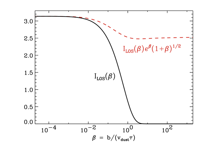
Figure 8: Numerically integrated values of $I_{\rm LOS}$ versus $\beta$ (solid black curve). The dominant exponential behavior is removed by multiplying $I_{\rm LOS}$ by the quantity $e^{\beta}\sqrt{1+\beta}$ (red dashed curve).

The visible-light flux $F_{\rm dust}$ emitted by dust grains (at a given distance $b$ away from the asteroid, and in a solid angle $\Omega$ that fills a WISPR pixel) can be computed and compared to the background sky flux. The total number of grains that contribute to this quantity is the product of the column density $N(b)$ and the cross-sectional area of one pixel as viewed by the spacecraft. If the spacecraft–asteroid distance $d$ is assumed to be much larger than the impact parameter $b$, the relevant cross-sectional area can be estimated to be $\Omega d^{2}$. Thus, if a single dust grain emits a visible-light flux $F_{1}$, the total flux in the pixel is given by

$$F_{\rm dust}\,=\,F_{1}\,N(b)\,\Omega d^{2}\,\,.$$ (21)

The calculation of $F_{1}$ was done using the equations in Section 3 and the assumption that each dust grain is essentially a “tiny asteroid” with a comparable albedo to its parent body.

At any time during an encounter between an asteroid and SPP, we can compute $F_{\rm dust}$ over a range of trial values of the impact parameter $b$. It is then possible to solve for a representative observed coma extent ($b_{\rm coma}$) that is the distance at which $F_{\rm dust}$ is equal to a threshold sky background flux. That sky flux was given by $10^{-4}F_{Z}$, which was determined in Section 3 to be the practical limit in modern-day heliospheric imagers for resolving small features from a large-scale background (DeForest et al., 2011). The quantity $F_{Z}$ depends on the elongation angle $\varepsilon$ and the SPP heliocentric distance $r_{p}$. Thus, the derived value of $b_{\rm coma}$ is observer-dependent and not intrinsic to the asteroid.

In the limiting case of $\beta\ll 1$, the dimensionless integral $I_{\rm LOS}$ approaches a constant value of $\pi$. Thus, the solution for the observed coma size can be written as

$$b_{\rm coma}\,\approx\,\left(\frac{F_{1}}{10^{-4}\,F_{Z}}\right)\,\pi R_{a}^{2}\,n_{d0}\,\Omega d^{2}\,\,\,.$$ (22)

The above expression was used as a validation for the full numerical solution in the limit of $b_{\rm coma}\ll v_{\rm dust}\tau$.

The model described above has three parameters that still have not yet been specified: $\cal M$, $v_{\rm dust}$, and $a$. We will use the Jewitt et al. (2013) measurement of $b_{\rm coma}=2.5\times 10^{5}$ km for Phaethon at its perihelion in order to constrain them. Plausible ranges of variability for these parameters are given as follows:

1. The dust-to-gas mass ratio ${\cal M}$ has been discussed above. Comet observations appear to give values of ${\cal M}\sim 1$ (A’Hearn et al., 1995; Sanzovo et al., 1996; Kolokolova et al., 2007), and recent high-quality measurements of comet 67P/Churyumov-Gerasimenko indicate values between 3 and 10 (Rotundi et al., 2015; Fulle et al., 2016). Measurements for active asteroids do not yet exist. Thus, with no firm firm observational guidance, we will vary ${\cal M}$ widely over seven orders of magnitude, between values of $10^{-3}$ and $10^{4}$.

2. The grain velocity $v_{\rm dust}$ can be parameterized as a ratio $\xi=v_{\rm dust}/v_{\rm gas}$, since $v_{\rm gas}$ is known from the sublimation model. Delsemme and Miller (1971) found that escaping gas molecules eventually accelerate to an asymptotic speed of $v_{\rm gas}\approx 1.8\,\bar{v}$. Thus, we specify $v_{\rm dust}$ as a function of $\bar{v}$ and $\xi$. For asteroids in the inner heliosphere, the temperatures shown in Figure 5(b) indicate $v_{\rm gas}\approx 0.3$–1 km s^-1. Comet observations tend to show that $v_{\rm gas}$ is a practical upper limit for $v_{\rm dust}$ (e.g., Waniak, 1992; Hughes, 2000; Prialnik et al., 2004; Beer et al., 2006; Bonev et al., 2008; Jewitt, 2012; Ishiguro et al., 2016). However, $v_{\rm dust}$ can take on a range of smaller values as well. A lower limit on $v_{\rm dust}$ is the escape velocity $v_{\rm esc}=(2GM_{a}/R_{a})^{1/2}$, which is typically between $10^{-4}$ and $10^{-3}$ km s^-1 for the asteroids considered here. Thus, we will assume a plausible range for the dimensionless velocity ratio of $10^{-4}<\xi<1$.

3. Astrophysical dust tends to exhibit a broad distribution of grain radii $a$ rather than any one specific value (Combi, 1994; Fulle, 2004). Observations of comets and the zodiacal light indicate particle sizes spanning the range from 0.1 $\mu$m to 10 cm (Fulle et al., 1993; Mann et al., 2004; Hörz et al., 2006; Kretke and Levison, 2015). Some models of dust loss from comets show a distinct anticorrelation between $a$ and $v_{\rm dust}$ (e.g., Finson and Probstein, 1968; Delsemme and Miller, 1971; Wallis, 1982), and this can be used to estimate the value of $a$ that maximizes the drift distance $R\approx v_{\rm dust}\tau$. However, observations often show grain sizes in excess of this putative maximum value (Tenishev et al., 2011). These models also underestimate $v_{\rm dust}$ by giving values only slightly larger than $v_{\rm esc}$, whereas observations often show a range of higher speeds extending up to $v_{\rm gas}$ (see above). In order to avoid undue dependence on these kinds of models, we allow the value of $a$ to vary freely between 0.01 $\mu$m and 10 cm.

With the above parameters ($\cal M$, $v_{\rm dust}$, $a$) varied freely and the other asteroid properties fixed for Phaethon at its perihelion, it is straightforward to compute $b_{\rm coma}$ using Equations (14)–(21) and compare the results to the observed value of $2.5\times 10^{5}$ km. An initial search of the parameter space yielded several clear constraints on the parameters. To match the observed coma size, models with $\xi\leq 1$ must have a dust-to-mass ratio of ${\cal M}>0.48$ and a representative grain size of $a<39$ $\mu$m. This latter constraint is in agreement with Jewitt et al. (2013), who inferred a grain radius of $a\approx 1$ $\mu$m for the particles producing the emission in the observed coma of Phaethon.

In order to help better constrain valid ranges of the free parameters, we searched for degeneracies (i.e., combinations of parameters that produced identical values of $b_{\rm coma}$). Figure 9 shows there is an extremely narrow “allowed” region in a two-dimensional cut through the solution space when the orthogonal axis parameters are defined as

$$C_{1}\,=\,\xi\,{\cal M}\,\,\,\,,\,\,\,\,\,\,\,\,C_{2}\,=\,a\,\xi^{-0.15}\,\,\,.$$ (23)

The points shown in Figure 9 are a subset of results from a Monte Carlo simulation of $10^{6}$ random trial solutions. The 5363 displayed points represent only those solutions that agree with the observed value of $b_{\rm coma}$ to within 1%.

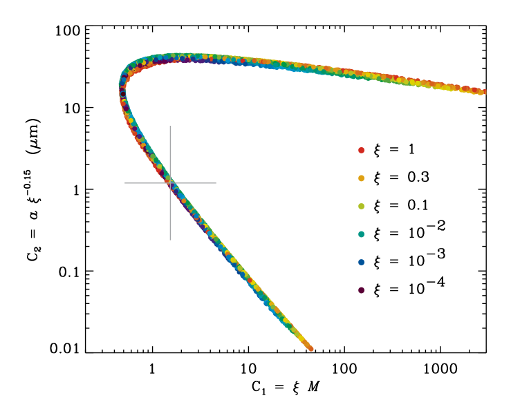
Figure 9: Two-dimensional parameter space of solutions to for $b_{\rm coma}$ that agree with observations of Phaethon at its perihelion. Symbol colors correspond to the values of $\xi$ (see legend), and the gray cross indicates values adopted for use with the SPP asteroid data: ${\cal M}=3$, $\xi=0.53$, $a=1$ $\mu$m.

Because all of the points shown in Figure 9 reproduce the SECCHI observations of $b_{\rm coma}$ for Phaethon at perihelion, we proceed by choosing one arbitrary set of values from those points to use in the models below. We presume the results for other asteroids at other heliocentric distances should scale similarly no matter the details of this choice. We follow Jewitt et al. (2013) by adopting $a=1$ $\mu$m as a mean dust grain radius. With that constraint, the other two parameters are seen to follow the relationship $\xi\approx 1.76/{\cal M}^{1.085}$. Optimized values of ${\cal M}=3$ and $\xi=0.53$ were thus chosen in order to maintain continuity with the cometary analogy; i.e., the empirical knowledge that ${\cal M}$ tends to be between 1 and 10 and that $v_{\rm dust}\approx v_{\rm gas}$ (or at least $v_{\rm dust}\gg v_{\rm esc}$) is often seen (e.g., Jewitt, 2012; Ishiguro et al., 2016).

5.2 Results for SPP Asteroid Encounters

Figure 10 shows some representative calculations of $b_{\rm coma}$ for the set of 97 closest-approach events described above (filled circles), and for a set of idealized asteroid properties and positions (solid curves). For these idealized curves, it was assumed that the three relevant bodies (the asteroid, SPP, and the Sun) were situated on the corners of an equilateral triangle. In other words, for each point along these curves, $r_{a}=r_{p}=d$ and $\alpha=\varepsilon=60^{\circ}$. For the 97 closest-approach events, these geometrical properties were extracted from the ephemerides discussed earlier. In cases when the dust ejected by an asteroid does not ever emit enough flux to exceed the observable sky background, we set $b_{\rm coma}$ to a lower limit of the asteroid radius $R_{a}$. This happens for all modeled cases at $r_{a}>0.3$ AU, which helps to justify our choice for disregarding asteroids with perihelia $q>0.3$ AU.

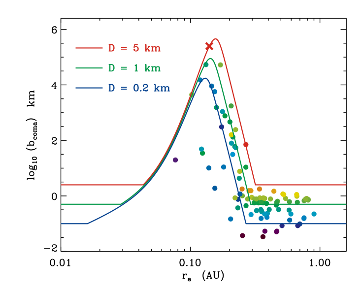
Figure 10: Distance dependence of the modeled observable dust cloud size $b_{\rm coma}$. Symbols correspond to the 97 closest-approach events, with colors corresponding to $H$ (i.e., asteroid diameter $D$) with the same scalings as in Figure 2. Curves correspond to grids of models with idealized geometrical configurations and fixed asteroid diameters (see text). The measured tail length of Phaethon at its perihelion (Jewitt et al., 2013) is shown with a red X symbol.

Note that there is a relatively finite range of heliocentric distances inside of which an asteroid is expected to emit grains that survive for thousands of kilometers and produce a bright dust coma. This range appears to be roughly $0.08<r_{a}<0.25$ AU. For asteroids closer to the Sun than about 0.05 AU, the sublimation rate $Z$ is so high that the grain lifetime $\tau$ is extremely short. Thus, the grains cannot reach large values of $b$ before they are destroyed. For asteroids further away from the Sun than about 0.3 AU, the sublimation rate $Z$ drops off to exceedingly small values. This allows any escaping grains to essentially “live forever,” but their number density $n_{d}$ is too low for their flux to compete effectively with the sky background.

Rather than limit the calculation to the small database of 97 closest-approach events, the entire ephemeris for each pairing of SPP with a given asteroid was processed to compute $b_{\rm coma}$ as a detailed function of time (i.e., at 0.1 day intervals). To compare directly with planned observations with WISPR, each value of $b_{\rm coma}$ was converted into a sky angle $\theta_{\rm coma}$ as observed from the vantage point of SPP,

$$\theta_{\rm coma}\,=\,\tan^{-1}\left(b_{\rm coma}/d\right)\,\,\,.$$ (24)

Because $b_{\rm coma}$ is a radius and not a diameter, a spherical dust cloud should have an observable angular extent of $2\theta_{\rm coma}$. However, we provide $\theta_{\rm coma}$ as a conservative lower limit in cases of efficient tail “blowback” behind the asteroid. A dust cloud is thus considered to be resolvable only when $\theta_{\rm coma}$ exceeds the size of a single WISPR pixel ($\theta\approx 1.45^{\prime}$).

Figure 11 shows the full set of cases with modeled values of $\theta_{\rm coma}$ that exceed 0.5^′ on the sky. The local maxima in $\theta_{\rm coma}$ occur neither at the times when $d=d_{\rm min}$ nor at the times when $r_{a}=q$. The large asteroid Phaethon shows up prominently with repeated peak values of $\theta_{\rm coma}$ between 10^′ and 26^′, no matter the location of SPP in the inner heliosphere. The smaller asteroids 137924, 155140, and 289227 each have one-time favorable events with $\theta_{\rm coma}>17^{\prime}$, but at other perihelion passes the angular extents are smaller. Figure 11 also makes clear that dust tail sizes greater than about 1^′ only tend to occur when asteroids fall between about 0.1 and 0.2 AU. Together with the results shown in Figure 10, this supports our choice to disregard asteroids with perihelia greater than 0.2–0.3 AU.

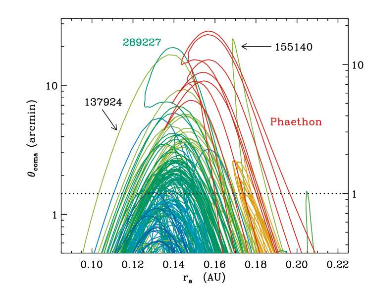
Figure 11: Evolution of the modeled dust-cloud angular size $\theta_{\rm coma}$ versus asteroid heliocentric distance for the full set of modeled encounters with SPP. Curve colors correspond to $H$ (i.e., asteroid diameter $D$) with the same scalings as earlier figures. The fiducial WISPR pixel size of 1.45^′ is noted with a dotted line.

Figure 12 shows essentially the same information that is in Figure 11, but plotted as a function of mission time $t$ instead of heliocentric distance. This shows that the individual episodes of large observable angular extent are limited in time and distributed sporadically through the SPP mission. There are 113 predicted maxima that exceed the assumed WISPR pixel size, corresponding to 24 distinct asteroids. Several of the maxima are closely spaced pairs or triplets, separated by hours to days, but most are isolated in time. The mean duration of an event (defined as the time spent with $\theta_{\rm coma}\geq 1.45^{\prime}$) is 1.39 days, but the events cover a range from 0.2 to 5.8 days. Table 3 lists the most promising 41 of these events (i.e., only those with $\theta_{\rm coma}\geq 3^{\prime}$) in order of mission time, and also gives the apparent magnitude $m_{V}$ of the parent asteroid and its heliocentric distance at the specific times of maximum $\theta_{\rm coma}$.

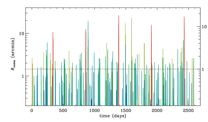
Figure 12: Evolution of the modeled dust-cloud angular size $\theta_{\rm coma}$ for various asteroids, versus mission time $t$ in days. Curve colors correspond to $H$ (i.e., asteroid diameter $D$) with the same scalings as earlier figures. The fiducial WISPR pixel size of 1.45^′ is noted with a dotted line.

Table 3: Predictions for large angular dust tail events, sorted by SPP mission time.

Time [days]	Name	$\theta_{\rm coma}$ [arcmin]	$m_{V}$	$r_{a}$ [AU]
187.90	394130	3.642	14.8	0.14501
230.71	394392	4.089	14.8	0.13994
234.80	394392	3.044	15.1	0.13974
246.21	374158	6.120	13.6	0.14030
293.41	137924	3.456	15.6	0.14530
336.51	Phaethon	10.813	12.1	0.15449
339.61	Phaethon	7.634	13.8	0.14855
593.10	137924	3.851	15.2	0.14837
770.76	374158	3.226	15.2	0.14133
790.45	394392	3.515	14.9	0.13631
857.14	2008 HW1	3.880	14.9	0.14726
860.34	Phaethon	12.624	11.8	0.15416
863.24	Phaethon	10.725	13.1	0.15071
893.13	137924	4.837	11.1	0.13828
897.13	289227	19.625	11.2	0.13989
897.23	137924	3.427	10.4	0.13533
899.03	289227	6.825	12.8	0.12748
899.83	289227	7.432	13.4	0.13680
994.40	2008 MG1	3.569	14.3	0.14497
994.60	2008 MG1	3.549	14.2	0.14520
1192.76	137924	5.927	13.1	0.14399
1210.85	2006 TC	4.175	14.7	0.14249
1291.13	374158	3.787	14.8	0.14196
1384.41	Phaethon	15.789	10.5	0.15016
1385.01	Phaethon	14.864	10.6	0.14506
1386.91	Phaethon	26.335	10.9	0.15667
1492.68	137924	17.238	9.6	0.13711
1493.88	2005 HC4	5.596	13.5	0.13366
1496.98	137924	9.264	12.2	0.14556
1590.26	155140	22.926	9.0	0.16850
1682.44	2013 HK11	3.211	12.5	0.15668
1709.33	394130	3.302	13.6	0.14533
1792.21	137924	5.994	14.2	0.14426
1796.71	137924	5.737	14.3	0.14657
1907.58	Phaethon	15.775	12.1	0.15692
2091.79	137924	4.344	15.0	0.14860
2328.12	374158	4.232	13.7	0.14082
2377.97	2008 HW1	3.645	14.4	0.14451
2391.48	137924	4.637	14.7	0.14859
2416.71	431760	6.875	13.1	0.14104
2431.22	Phaethon	24.707	11.1	0.15633

6 Discussion and Conclusions

The goal of this paper is to call the community’s attention to the likelihood that SPP will be well-positioned to observe mass loss from Mercury-crossing asteroids in the inner heliosphere. Specifically, we predict that there will be several times during the SPP mission when the WISPR instrument will be able to detect visible-light emission from the asteroids themselves and (in a few cases) from associated dust clouds that may subtend almost a degree of angular width on the sky. These observations could fill in a large gap between the properties of two heretofore distinct populations—active asteroids and sungrazing comets—and thus help complete the census of primordial solar system material.

Because of several ongoing uncertainties, many of the quantitative predictions made above may not remain valid for the actual SPP mission to commence in 2018. Specifically, the following four factors will need to be re-evaluated over the coming few years:

1. As noted in Section 2, if the spacecraft launch slips from its nominal date of July 31, 2018, the predicted time-dependent distances between SPP and the asteroids will be incorrect. The mission depends on multiple close encounters with Venus to adjust the trajectory into the desired elliptical orbit with a perihelion of 0.0459 AU. Fox et al. (2015) described a backup plan that involves a May 2019 launch plus one additional Venus gravity assist to bring SPP into an orbit similar to the baseline trajectory.

2. Many of the objects in our database of 97 Mercury-crossing asteroids have been discovered relatively recently. Thus, there may still be substantial uncertainties in their ephemeris parameters. Such errors would necessarily propagate into our predictions of the relative times and distances of encounters with SPP. Whether the improvement of these parameters would give rise to a larger or smaller number of favorable encounters remains to be seen. Nevertheless, the pace of asteroid discovery is likely to continue, and there may be dozens more possible targets discovered between now and 2018.

3. The predictions made above did not take into account that the WISPR instrument has a finite field of view and cannot see the entire sky. Some fraction of favorable encounters with asteroids may end up being hidden behind the SPP heat shield or other parts of the spacecraft. Thus, not every asteroid in listed Tables 1 and 3 will be observable at all times. These details need to be considered when constructing detailed observation plans, but they are beyond the scope of this paper.

4. The observability of any given asteroid and its surrounding dust cloud was computed using a threshold sky background of $10^{-4}F_{Z}$ (see, e.g., DeForest et al., 2011). It is possible that WISPR may contain sufficient improvements in photon counting or flat-fielding, relative to the SECCHI package on STEREO, that could allow even weaker signals to be extracted from the raw images.

However the above issues are resolved, there appears to be a high probability for a significant number of encounters between SPP and Mercury-crossing asteroids during times when the latter may be losing mass at $r_{a}<0.2$ AU. Details aside, the statistical distribution of events is likely to remain similar to what was computed in this paper.

In addition to refining the positional and temporal accuracy of the above predictions, there are also several ways that the mass loss modeling can be improved. Our assumption of constant values for $L$ and $\mu$ should be replaced by a more self-consistent (i.e., temperature dependent) description of specific ejected materials. This is particularly important because the computed rates are often in the exponentially dropping part of the sublimation curve (Figure 5), where small variations in the input parameters could change $Z$ by several orders of magnitude. Also, the spherically symmetric Haser (1957) model should be replaced by a full three-dimensional dynamical simulation of the ejected dust grains. If the escaping grains are swept back into a collimated tail, their number density may be up to an order of magnitude higher (and thus more easily observable when viewed from a favorable direction) than if they were spread out in a spherical cloud. Jewitt et al. (2011) estimated the sunward turnaround distance $s$ expected from grains of a given size. In cases where $s\ll b_{\rm coma}$ it would be most useful to apply such a three-dimensional correction to the density model. At the very least, the standard Finson and Probstein (1968) type of ballistic modeling should be done for the most promising encounters, in order to predict the tail orientations and geometries.

The idea of using inner heliospheric space probes as remote observatories for active asteroids should be expanded beyond just SPP. The Solar Orbiter mission (Müller et al., 2013; Bemporad et al., 2015) will reach a minimum perihelion distance of about 0.28 AU during a similar time-frame as SPP, but it will also leave the ecliptic plane to eventually reach inclination angles of order 30^∘. Sarli et al. (2015) proposed a mission to visit Phaethon and associated asteroids (155140) 2005 UD and (225416) 1999 YC, which would explore the origins of the Geminid meteor stream and study the physics of comet/asteroid transition objects. Near-Earth asteroid flyby or rendezvous missions with infrared spectro-imagers (Groussin et al., 2016) could also improve our knowledge of the physics of regolith loss in a hot thermal environments. Lastly, any spacecraft that comes close enough to fly through the dust tail of an active asteroid would put unprecedented constraints on the properties of the ejected grains, thus allowing a comparison of similarities and differences to dust ejected by comets (see, e.g., Kissel and Krueger, 1987; Mann and Czechowski, 2005; Neugebauer et al., 2007; Della Corte et al., 2015).