Comparison of analytic and numerical bond-order potentials for W and Mo

Abstract

Bond-order potentials (BOPs) are derived from the tight-binding (TB) approximation and provide a linearly-scaling computation of the energy and forces for a system of interacting atoms. While the numerical BOPs involve the numerical integration of the response (Green’s) function, the expressions for the energy and interatomic forces are analytical within the formalism of the analytic BOPs. In this paper we present a detailed comparison of numerical and analytic BOPs. We use established parametrisations for the bcc refractory metals W and Mo and test structural energy differences; tetragonal, trigonal, hexagonal and orthorhombic deformation paths; formation energies of point defects as well as phonon dispersion relations. We find that the numerical and analytic BOPs generally are in very good agreement for the calculation of energies. Different from the numerical BOPs, the forces in the analytic BOPs correspond exactly to the negative gradients of the energy. This makes it possible to use the analytic BOPs in dynamical simulations and leads to improved predictions of defect energies and phonons as compared to the numerical BOPs.

I Introduction

Refractory metals exhibit properties that make them unique compared to other metals. They have an exceptionally high melting point, excellent strength at high temperatures as well as good wear, corrosion and abrasion resistance. Moreover, they show very high hardness and good electrical and heat conducting properties. Here we focus on the bcc refractory metals W and Mo. Tungsten and its alloys are used for light-bulbs and filaments and in the future possibly as plasma-facing wall material in fusion reactors. Molybdenum is often used as alloying element in high-strength steels (up to 8%) and in superalloys (Ni- or Co-based) in order to increase the melting temperature. One of the more recent applications are bulk metallic glasses with exceptionally high glass-transition and crystallisation temperatures. Zhang et al. (2005)

Modelling the mechanical behaviour of refractory metals requires to account for microstructural defects, such as dislocations and grain boundaries as well as secondary phase precipitates. Empirical potentials, such as Finnis-Sinclair Finnis and Sinclair (1984) or the embedded-atom method (EAM) Daw and Baskes (1984), only partly capture the nature of bonding mediated by d electrons in bcc transition metals Gröger et al. (2008). Tight-binding (TB) methods, as approximate electronic structure methods, are attractive because they can treat large systems and at the same time offer an understanding of the underlying physical processes. The bond-order potentials (BOPs) provide a linear scaling approximate solution to the TB problem Pettifor (1989); Aoki (1993); Horsfield et al. (1996a); Drautz and Pettifor (2006, 2011); Hammerschmidt and Drautz (2009); Hammerschmidt et al. (2009); Finnis (2007). BOPs have proved to be particularly effective for simulating properties of dislocations Girshick et al. (1998a, b); Vitek et al. (2004); Mrovec et al. (2004, 2007); Katzarov et al. (2007); Gröger et al. (2008); Katzarov and Paxton (2009) or in explaining the origin of brittle cleavage in iridium Cawkwell et al. (2005, 2006).

While the properties of dislocations predicted from BOPs are typically more robust and reliable than predictions from empirical potentials, a recent study Cereceda et al. (2013) deemed numerical BOPs as not suitable for finite temperature dynamical simulations because of a mismatch between the forces and the negative gradients of the energy. Analytic BOPs Drautz and Pettifor (2006, 2011); Seiser et al. (2013), in contrast, provide forces that exactly match the negative gradients of the energy.

In this paper we present a detailed comparison between analytic and numerical BOPs. We show that the energies predicted using analytic BOPs and numerical BOPs are essentially equivalent, such that existing parametrisations of numerical BOPs may directly be used in dynamical simulations with the analytic BOPs. In section  II we briefly review the main differences between the numerical and analytic BOPs. In section III the BOPs are compared by using the electronic density of states, structural energy differences, point defect formation energies, structural transformation paths and phonon spectra.

II Methodology

II.1 Tight Binding

The derivation of BOPs starts from the TB approximation that expresses the eigenfunctions $\psi_{n}$ of the Schrödinger equation

$$\hat{H}\psi_{n}=E_{n}\psi_{n}\,,$$ (1)

in a minimal basis of orbitals $\alpha$ centred on atoms $i$

$$|\psi_{n}\rangle=\sum\limits_{i\alpha}c_{i\alpha}^{(n)}|i\alpha\rangle\,.$$ (2)

For an orthonormal basis, the eigenvalues $E_{n}$ and the coefficients $c_{i\alpha}^{(n)}$ of the eigenfunctions $\psi_{n}$ are determined by solving the secular equation

$$\sum\limits_{j\beta}H_{i\alpha j\beta}c_{j\beta}^{(n)}=E_{n}c_{i\alpha}^{(n)}\,.$$ (3)

The matrix elements $H_{i\alpha j\beta}$ are typically expressed as functions of the interatomic distance. The diagonalisation of the Hamiltonian matrix

$$H_{i\alpha j\beta}=\langle i\alpha|\hat{H}|j\beta\rangle\,,$$ (4)

is the computationally most demanding part of TB calculations. In the TB bond model Sutton et al. (1988); Drautz and Pettifor (2011), the binding energy of a d-valent, charge neutral and non-magnetic material is given as the sum over the covalent bond energy $U_{\mathrm{bond}}$ and the repulsive energy $U_{\mathrm{rep}}$

$$U_{B}=U_{\mathrm{bond}}+U_{\mathrm{rep}}\,.$$ (5)

The bond energy $U_{\mathrm{bond}}$ can be expressed in onsite and intersite representation. Both representations are equivalent but offer different views on bond formation. The onsite representation is based on the atom-based local density of states $n_{i\alpha}$ on atom $i\alpha$,

$$n_{i\alpha}(E)=\sum\limits_{n}\left|c_{i\alpha}^{(n)}\right|^{2}\delta(E-E_{n})\,.$$ (6)

The intersite representation is expressed in terms of the bond-order $\Theta_{i\alpha j\beta}$ or the density matrix $\rho_{i\alpha j\beta}$ between orbital $\alpha$ on atom $i$ and orbital $\beta$ on atom $j$ and is given by the sum over occupied states

$$\Theta_{i\alpha j\beta}=2\rho_{i\alpha j\beta}=2\sum\limits_{n}^{\mathrm{occ}}c_{i\alpha}^{*(n)}c_{j\beta}^{(n)}\,.$$ (7)

The bond energy in onsite and intersite representation is given by

$$U_{\mathrm{bond}} = 2\sum\limits_{i\alpha}\int\limits^{E_{\mathrm{F}}}\left(E-E_{i\alpha}\right)n_{i\alpha}(E)dE$$

$$= \sum\limits_{i\alpha\neq j\beta}\Theta_{i\alpha j\beta}H_{i\alpha j\beta}\,,$$

where $E_{\mathrm{F}}$ is the Fermi level and $E_{i\alpha}$ = $H_{i\alpha i\alpha}$ are the diagonal elements of the Hamiltonian matrix. An in-depth discussion and interpretation of the bond order for molecules and solids is given in Refs. Finnis, 2007; Pettifor, 1995.

II.2 Bond-Order Potentials

The p-th moment of the local density of states $n_{i\alpha}(E)$ is given by Ducastelle and Cyrot-Lackmann (1970); Horsfield et al. (1996a)

$$\mu^{(p)}_{i\alpha} = \int E^{p}n_{i\alpha}(E)dE=\langle i\alpha|\hat{H}^{p}|i\alpha\rangle$$

$$= \sum\limits_{j_{1}\beta_{1},j_{2}\beta_{2}...j_{p-1}\beta_{p-1}}H_{i\alpha j_{1}\beta_{1}}H_{j_{1}\beta_{1}j_{2}\beta_{2}}...H_{j_{p-1}\beta_{p-1}i\alpha}\,.$$

Using the last equality one understands the p-th moment of the local density of states as a closed loop of p hops along neighbouring atomic sites. The local density of states $n_{i\alpha}(E)$ can be reconstructed from its moments $\mu^{(p)}_{i\alpha}$ by making use of the recursion method Haydock (1980a, b) with the on-site Green’s function $G_{00}(E)$ expressed as a continued fraction

$$G_{00}(E)=\cfrac{1}{E-a_{0}-\cfrac{b_{1}^{2}}{\ddots-\cfrac{\ddots}{E-a_{\infty}-\cfrac{b_{\infty}^{2}}{\ddots}}}}$$ (10)

with recursion coefficients $a_{i}$ and $b_{i}$. The recursion coefficients may be computed from the moments of the density of states. Typically, for a single band, one calculates the first few recursion coefficients, equivalent to the first $m_{\rm max}$ moments, and estimates the following recursion coefficients as $a_{\infty}$ and $b_{\infty}$, independent of $i$. Because the part of the continued fraction that involves only $a_{\infty}$ and $b_{\infty}$ can be evaluated to a square-root analytically Horsfield et al. (1996a), this is referred to as the square-root terminator.

The local density of states is related to the Green’s function Horsfield et al. (1996a)

$$n_{i\alpha}(E)=-\frac{1}{\pi}\lim_{\epsilon\to 0}\mathrm{Im}\{G_{i\alpha i\alpha}(E+i\epsilon)\}\,.$$ (11)

From Eq. II.1 one can then calculate the bond energy by numerical integration, which is referred to as numerical BOP. The forces are obtained approximately by using the Hellmann-Feynman theorem. The numerical integration is one of the computational bottlenecks of such calculations. In numerical BOP, an effective electronic temperature $T_{e}$ is introduced in order to improve the convergence of the bond-order expansion and to obtain a better agreement between the approximate Hellmann-Feynman forces and the true forces, i.e., the negative gradients of the energy Horsfield et al. (1996a); Girshick et al. (1998a). As the introduction of the electronic temperature is an approximation on top of the numerical BOP expansion, in the following we use an electronic temperature of $k_{B}T_{e}=$ 0.001 eV to keep the influence on binding energies and forces as small as possible. This value is smaller than the typically used $k_{B}T_{e}=$ 0.3 eV, but still provides numerical stability and very good agreement of the bond energies from numerical and analytic BOPs.

In the analytic BOPs, the density of states is expanded using Chebyshev polynomials of the second kind $U_{m}(\epsilon)$ Drautz and Pettifor (2006, 2011),

$$n_{i\alpha}(\epsilon) = \frac{2}{\pi}\sqrt{1-\epsilon^{2}}\Bigg{[}\sum\limits_{m=0}^{m_{\rm{max}}}g_{U}^{(m)}\sigma_{i\alpha}^{(m)}U_{m}(\epsilon)$$

$$+\sum\limits_{m_{\rm{max}}+1}^{m_{\rm{exp}}}g_{U}^{(m)}\sigma_{i\alpha}^{(m)}U_{m}(\epsilon)\Bigg{]}\,.$$

The expansion coefficients $\sigma_{i\alpha}^{(m)}$ are obtained from the moments ${\mu}_{i\alpha}^{(p)}$. In analogy to the numerical BOPs, only the first few expansion coefficients corresponding to $m_{\rm max}$ moments are explicitly computed. The remaining expansion coefficients up to $m_{\rm exp}$ are obtained from the square-root terminator Seiser et al. (2013). The terminator coefficients $a_{\infty}$ and $b_{\infty}$ are also used to ensure that the density of states is contained in the band $-1\leq\epsilon\leq+1$, with $\epsilon=\frac{E-a_{\infty}}{2b_{\infty}}$. We approximate the values of $a_{\infty}$ and $b_{\infty}$ from the upper and lower bounds of the energy spectra,

$$E_{\rm{min}}=a^{\rm{min}}-2b^{\rm{max}}\quad{\rm and}\quad E_{\rm{max}}=a^{\rm{max}}-2b^{\rm{max}}\,,$$ (13)

and therefore

$$a_{\infty}=\frac{E_{\rm{max}}+E_{\rm{min}}}{2}\quad{\rm and}\quad b_{\infty}=\frac{E_{\rm{max}}-E_{\rm{min}}}{4}\,.$$ (14)

The damping factors $g_{U}^{(m)}$ vary smoothly from one at $m=0$ to zero at $m=m_{\rm exp}$ (see Fig. 2 in Ref. Seiser et al., 2013) and prevent Gibbs ringing in the expansion such that the resulting density of states is always strictly positive Seiser et al. (2013); Silver et al. (1996).

II.3 Functional form and parametrisation

Our comparison between analytic and numerical BOPs is based on previously developed parametrisations for Mo Mrovec et al. (2004) and W Mrovec et al. (2007). The bond energy $U_{\mathrm{bond}}$ (Eq. II.1) in the d-valent TB model is determined by the matrix elements $H_{i\alpha j\beta}$ (Eq. 4) that are expressed in terms of two-centre Slater-Koster Slater and Koster (1954) bond integrals $\beta(R)$ and parametrised by the Goodwin-Skinner-Pettifor (GSP) function Goodwin et al. (1989)

$$\beta(R)=\beta(R_{0})\Big{(}\frac{R_{0}}{R}\Big{)}^{n_{a}}\mathrm{exp}\Big{\{}n_{b}\Big{[}\Big{(}\frac{R_{0}}{R_{c}}\Big{)}^{n_{c}}-\Big{(}\frac{R}{R_{c}}\Big{)}^{n_{c}}\Big{]}\Big{\}}\,.$$ (15)

where $R_{0}$ is the first nearest neighbour distance in bcc. The long-range tail of the GSP function is smoothly forced to zero by a cut-off function between $R_{\rm{tail}}$ and $R_{\rm{cut}}$. In the interval $R_{\rm{cut}}$ - $R_{\rm{tail}}$ the GSP function is replaced by a fifth-order polynomial that guarantees continuous second derivatives. The number of d electrons $N_{d}$ is taken as $N_{d}$ = 4.2 for both, Mo and W. An environmental repulsive term $U_{\mathrm{rep}}^{\mathrm{env}}$ is introduced in order to account for a correct description of the Cauchy pressure and is modelled by a Yukawa-like many-body environmentally dependent repulsive term Nguyen-Manh et al. (2008),

$$U_{\mathrm{rep}}^{\mathrm{env}}=\frac{1}{2}\sum\limits_{i,i\neq j}\frac{B}{r_{ij}}\mathrm{exp}[-\lambda_{ij}(r_{ij}-2r_{\mathrm{core}})]\,,$$ (16)

where

$$\lambda_{ij}=\frac{1}{2}(\lambda_{i}+\lambda_{j})\,,$$ (17)

and

$$\lambda_{i}=\lambda_{0}+\Big{[}\sum\limits_{k\neq i}C\mathrm{exp}(-\nu R_{ik})\Big{]}^{1/m}\,.$$ (18)

Just like for the bonding integrals we are using a fifth-order polynomial as cutoff function for the Yukawa-like term that acts on equations 16 and 18. The pair potential term $U_{\mathrm{rep}}^{\mathrm{pair}}$ accounts for the repulsive short-range character of the atomic interactions. It is represented by a cubic spline,

$$U_{\mathrm{rep}}^{\mathrm{pair}}=\frac{1}{2}\sum\limits_{i,i\neq j}\sum\limits_{k=1}^{4}A_{k}(R_{k}-R_{ij})^{3}\,,$$ (19)

with parameters chosen such that the pair potential vanishes between the second and third nearest neighbour. For this reason, no cut-off function needs to be applied.

II.4 Computational details

The calculations presented in the following were carried out with OXON Horsfield et al. (1996a, b) and BOPfox Hammerschmidt et al. . Both packages provide a TB kernel and we confirmed that the TB results using OXON and BOPfox are in excellent agreement. For the TB calculations presented in the following we used a Monkhorst-Pack k-point mesh Monkhorst and Pack (1976) and the tetrahedron method Blöchl et al. (1994) for integrating the Brillouin zone. For all TB calculations we used a k-point mesh of 30$\times$30$\times$30 which is sufficient also for the calculations along the deformation paths, where the symmetry is lowered compared to bcc. For the BOP calculations, we used OXON for the numerical BOP and BOPfox for the analytic BOP calculations. Both BOPs use the same TB model with the functional form given in section II.3 and parameters given in Refs. Mrovec et al., 2004, 2007. Therefore, the contributions of the repulsive energies are identical in analytic BOP (using BOPfox) and numerical BOP (using OXON), only the bond energy is treated with different formalisms.

III Comparison of analytic and numerical BOP

III.1 Density of states

In Fig. 1, we compare the density of states of bcc W as obtained with the numerical BOP using 9 moments and with the analytic BOP using $m_{\rm{max}}=9$ moments and $m_{\rm{exp}}=200$ to the TB reference calculations.

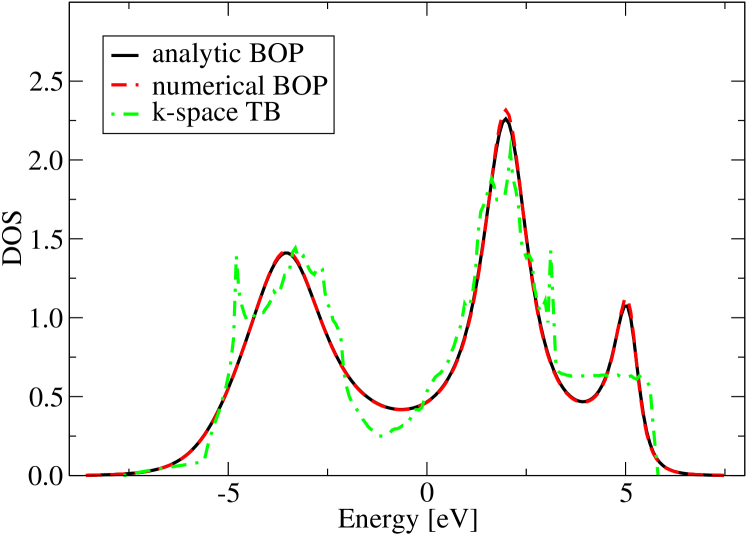
Figure 1: Density of states of tungsten calculated using different approximations.

We find excellent agreement between the numerical BOP and the analytic BOP. Nine moments in the BOP calculations are sufficient to reproduce the central features of the TB density of states, particularly the positions of the bonding and anti-bonding peaks and the pseudo gap. This number of moments was also used in the original parametrisations Mrovec et al. (2004, 2007) and previously shown to be sufficient for describing structural stability in transition metals Seiser et al. (2011). The following tests were carried out with the same numbers of moments.

III.2 Structural stability

Experimental and calculated properties of the bcc ground state for Mo and W are summarised in Tab. 1.

		expt	analytic BOP	numerical BOP	TB
Mo	$C_{11}$	2.901	2.974	2.972	3.181
	$C_{12}$	1.008	0.931	0.946	0.825
	$C_{44}$	0.680	0.603	0.730	0.422
	$E_{\rm{coh}}$	-6.82	-6.79	-6.75	-6.80
	$a_{0}$	3.147	3.147	3.147	3.147
W	$C_{11}$	3.261	3.320	3.311	3.535
	$C_{12}$	1.276	1.195	1.213	1.083
	$C_{44}$	1.002	0.911	1.045	0.704
	$E_{\rm{coh}}$	-8.90	-8.89	-8.84	-8.90
	$a_{0}$	3.165	3.165	3.165	3.165

Table 1: Elastic constants $C_{11}$, $C_{12}$ and $C_{44}$ [eV/ų], cohesive energies [eV/atom] and lattice constants [Å] as obtained from experiment (see references in Ref. Finnis and Sinclair, 1984), from analytic and numerical BOP and from TB.

The energies for analytic and numerical BOP as well as for TB as a function of atomic volume are shown in Fig. 2.

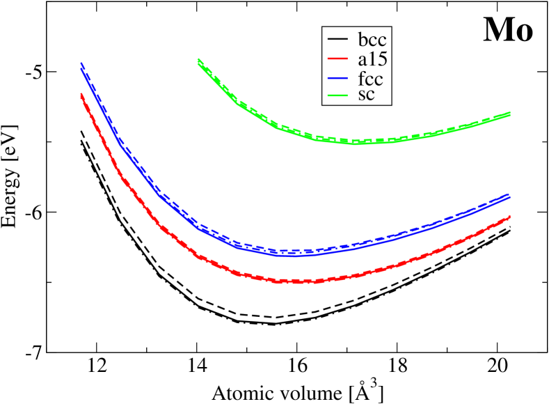
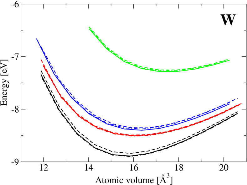
Figure 2: Energy vs. volume curves. Full lines represent analytic BOP, dashed lines numerical BOP and dot-and-dash lines TB.

For both analytic and numerical BOP, the elastic constants are determined by fitting a fifth-order polynomial to the energy versus deformation data. From Tab. 1 one can see a good agreement between analytic and numerical BOP values of elastic parameters and cohesive energies with a slightly better match of the analytic BOP data to the TB reference than the numerical BOP. Figure 2 shows that for both Mo and W the analytic and numerical BOPs are in a very good agreement, predicting essentially the same energetics of the structures presented here, once more with a slightly better match of the TB data by analytic BOP as compared to numerical BOP.

III.3 Transformation paths

We consider several transformation or deformation paths in bcc. We calculate the energy as a function of the deformation parameter and compare it to TB. A more detailed description of the geometries of these paths can be found in literature Paidar et al. (1999); Luo et al. (2002). Various deformation paths were studied in relation to the stability of the higher energy phases and extended defects Wang and Sob (1999); Wang et al. (1997).

III.3.1 Tetragonal deformation path

The tetragonal deformation path follows loading of bcc along the [001] direction with the deformation parameter $c/a$. Here $c$ is the lattice parameter along [001] and $a$ along [100] a [010]. The volume of the unit cell is conserved along this path. In a coordinate system with [001] and [100] parallel to the $z$ and $x$ axis, the only non-zero components of the Green-Lagrangian strain tensor for this deformation path are

$$\epsilon_{11}=\epsilon_{22}=\frac{a^{2}-a_{0}^{2}}{2a_{0}^{2}},\quad\epsilon_{33}=\frac{c^{2}-a_{0}^{2}}{2a_{0}^{2}}\,,$$ (20)

where $a_{0}$ is a lattice parameter of perfect bcc. Along this transformation path, $c/a$=1 and $c/a$=$\sqrt{2}$ correspond to bcc and fcc, respectively. These are visible as minimum (bcc) and maximum (fcc) in the binding energy along the transformation path as compiled in Fig. 3.

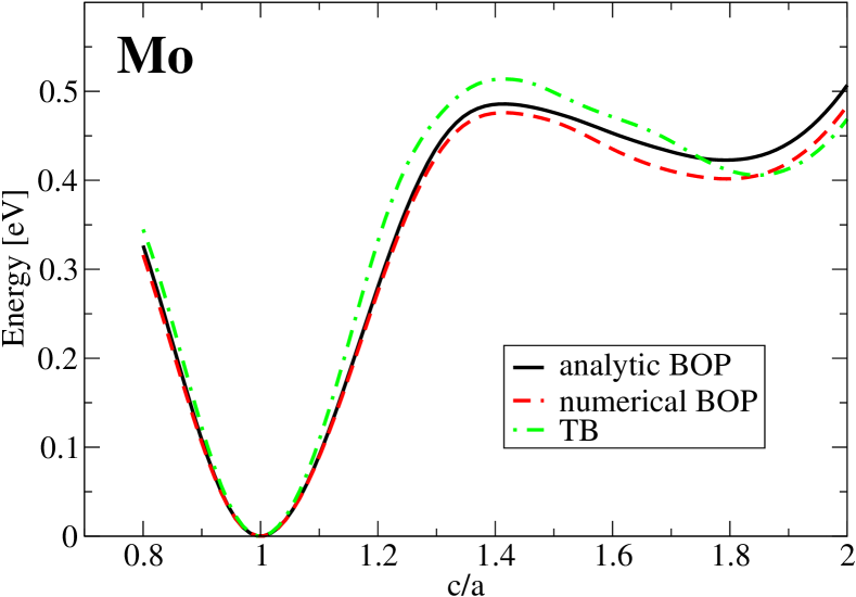
Figure 3: Binding energy along the tetragonal deformation path. The minimum at $c/a$ = 1 corresponds to bcc, the maximum at $c/a$=$\sqrt{2}$ to fcc.

The agreement between analytic and numerical BOP as well as the reference TB calculations is very good in the whole range of deformations. We note that the region around the global minimum (bcc) is related to the tetragonal shear modulus $C^{{}^{\prime}}$. Importantly, we find the correct positions and energies of the local maximum for fcc (symmetry dictated) and the local minimum (not dictated by symmetry) at $c/a$ = 1.6-1.8.

III.3.2 Trigonal deformation path

The trigonal deformation path represents a deformation of bcc with loading/compression along [111]. The atomic volume along the path is conserved and the trigonal deformation connects bcc, sc and fcc at $p$=1, $p$=2 and $p$=4, respectively, see Fig. 4.

Figure 4: Binding energy along the trigonal deformation path. The minimum at $p$ = $1$ corresponds to bcc, the maxima at $p$=$2$ and $p$=$4$ to fcc and sc, respectively.

The agreement between analytic BOP, numerical BOP and TB is excellent along the deformation path including the local maximum at $p=4$. The curvature around the global energy minimum at $p$=1 is related to the trigonal (or rhombohedral) shear modulus $C_{44}$.

III.3.3 Hexagonal deformation path

The hexagonal deformation path connects bcc with the hexagonal closed-packed (hcp) structure. It combines loading with a linearly coupled shuffling of the atomic planes Paidar et al. (1999); Mrovec et al. (2004). In our representation, $p$ = 0 and $p$ = 1 represent bcc and hcp, respectively. From our results compiled in Fig. 5 we see that the agreement between analytic and numerical BOP and TB is very good along the full transformation path.

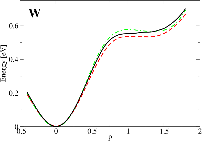
Figure 5: Binding energy along the hexagonal deformation path. The minimum at $p$ = $0$ corresponds to bcc, the maximum at $p$=$1$ to hcp.

III.3.4 Orthorhombic deformation path

The orthorhombic deformation path connects two bcc structures with one symmetry dictated maximum that corresponds to a body-centred tetragonal (bct) lattice. This deformation is described by a rotation of the coordinate system to [110], [$\bar{1}$10] and [001], respectively. Then the bcc structure is simultaneously elongated along [001] and compressed in the [110] direction. The non-vanishing components of the corresponding Lagrangian strain tensor are

$$\epsilon_{11}=\frac{p^{-1}-1}{2},\quad\epsilon_{33}=\frac{p-1}{2}\,.$$ (21)

Values of $p=1$ and $p=2$ correspond to bcc, $p=\sqrt{2}$ to the bct structure. Our results shown in Fig. 6 show very good agreement between analytic and numerical BOP and TB.

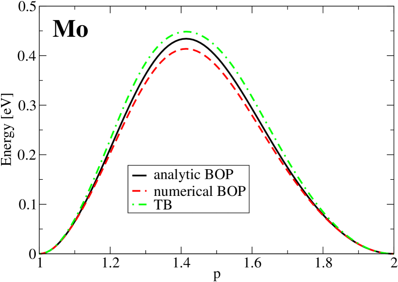
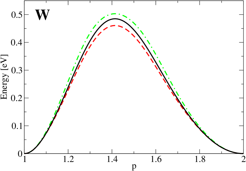
Figure 6: Binding energy along the orthorhombic deformation path. The minima at $p$ = $1$ and $p$ = $2$ correspond to bcc, the maximum at $p$=$\sqrt{2}$ to bct.

III.4 Point defects

We compare the formation energies of (i) a single vacancy in bcc and (ii) self-interstitial atoms (SIAs) in bcc. The SIAs are labelled as [001], [111] and [110] according to the Miller indices of the corresponding crystallographic direction as shown in Fig. 7.

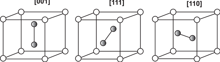
Figure 7: Self-interstitial atom configurations in bcc.

The sequence of energetic stability of the SIAs in bcc transition metals was identified only in recent years. Ackland and Thetford Ackland and Thetford (1987) have found (using the semi-empirical Finnis-Sinclair potential) the [110] configuration to be most stable for all bcc TMs with the exception of W. Later on, Han et al. Han et al. (2002) predicted on the basis of density-functional theory (DFT) calculations the [111] configuration to have the lowest formation energy for Mo and V. For iron, the [110] SIA is most stable according to DFT Domain and Becquart (2001); Fu et al. (2004) and TB calculations Liu et al. (2005). Nguyen-Manh et al. Nguyen-Manh et al. (2006) and Derlet et al. Derlet et al. (2007) have undertaken a systematic DFT study of SIA for all 5B and 6B group bcc transition metals, with the conclusion that in all cases the [111] SIA is the most stable defect. This discrepancy between DFT and empirical potentials is related to the binding behaviour at short distances: when the metallic material is isotropically compressed, the kinetic energy of the electrons and the ion-ion repulsion increases. In most of the semi-empirical schemes this is accounted for only by adjusting the pairwise potential, which is then overestimated and gives rise to a steep increase at short interatomic distances. In SIA configurations, however, short bond lengths are present without the corresponding significant change in volume. This leads to the discrepancy in the formation energies of interstitials, as pointed out by Han et al. Han et al. (2002). The TB model employed here has limitations in describing the short-range interaction appropriately, as pointed out earlier Mrovec et al. (2007).

For the SIAs calculations we converged the energies w.r.t. the cell size. For both vacancy and interstitials we used a 6$\times$6$\times$6 bcc supercell with 431 atoms for the vacancy and 433 atoms for the SIAs. Our results using analytic BOPs, numerical BOPS, and TB are compiled and compared with experimental data and with DFT results of Nguyen-Manh et al. Nguyen-Manh et al. (2006) in Tab. 2.

		expt Kittel (1976); Erhart et al. (1991)	DFT Nguyen-Manh et al. (2006)	analytic	numerical	TB
				BOP	BOP
Mo	vac	2.6-3.2	2.96	2.59	2.43	2.63
	[111]		7.42	8.70	7.92	8.37
	[110]		7.58	6.48	6.28	6.41
	[001]		9.00	9.54	8.59	9.31
W	vac	3.5-4.1	3.56	4.15	3.98	4.17
	[111]		9.55	11.92	10.81	11.45
	[110]		9.84	9.28	9.17	9.08
	[001]		11.49	12.63	11.71	11.97

Table 2: Formation energies of vacancies and interstitials in bcc Mo and W in units of [eV] obtained from experiment Kittel (1976); Erhart et al. (1991), DFT Nguyen-Manh et al. (2006) and BOP/TB calculations.

The differences between numerical and analytic BOP for the SIA formation energies are of two origins. First, there are differences in the total energy for the same atomic configuration, as illustrated in Sec. III.2 and III.3. Second, there are differences in the relaxed structures of the SIA configurations as a consequence of differences in the forces for the same atomic configuration. In order to illustrate the difference between the computed forces we determine the forces using the analytic BOP and the numerical BOP formalism and compute the numeric derivative of the energy. We evaluate the force on a central atom of a two-atom bcc unit cell for different shifts along the x-axis by up to 0.05 Å as summarised in Fig. 8.

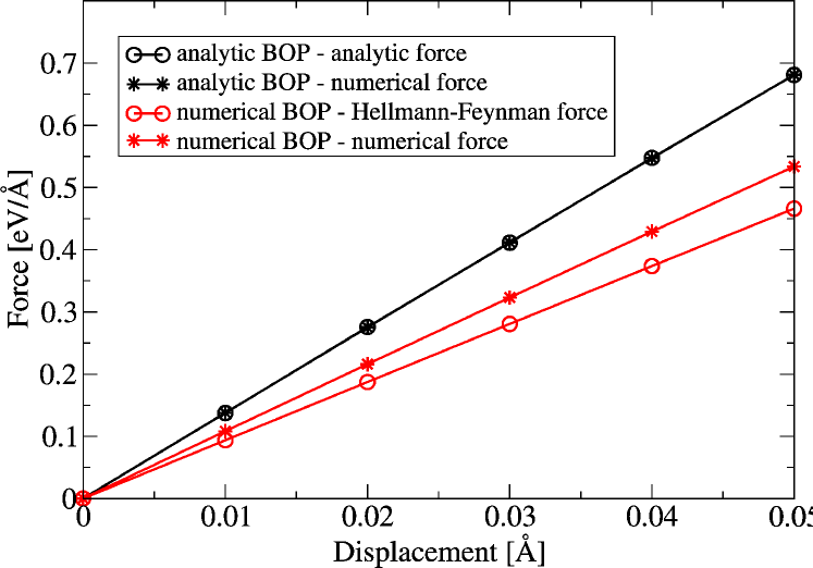
Figure 8: Absolute values of the x-component of the force on the central atom in the bcc unit cell as a function of the displacement of the atom in x-direction.

The numerical forces were obtained using centred finite differences with steps of $\Delta=\pm 10^{-6}$ Å. For the numerical BOPs we observe a significant deviation of the approximate Hellmann-Feynman forces and the numerical forces. This inconsistency is the origin of the comparably large deviations of the numerical BOP from the TB results of SIA formation energies and a limitation for the application of numerical BOPs in dynamic simulations Cereceda et al. (2013). For the analytic BOP we find an exact agreement of the analytic and numerical forces. This illustrates that the forces in the analytic BOP formalism are strictly consistent with the derivative of the binding energy. The consistent treatment of energy and forces in the analytic BOP, together with the linearly-scaling computation of energy and forces, enables large-scale molecular-dynamics simulations.

III.5 Phonons

We furthermore calculated the phonon dispersion curves for Mo and W and compare our results to the available experimental data. We use 216-atom supercells and the Phon software Alfè (2009) that employs the small displacement method. Our setup ensures that the values of the force constant matrices vanish for atoms that are distant from the displaced atom. Our calculated phonon dispersion curves for three high-symmetry directions in the Brillouin zone of bcc, $\Gamma$-H, $\Gamma$-N and $\Gamma$-P-H, are shown in Fig. 9.

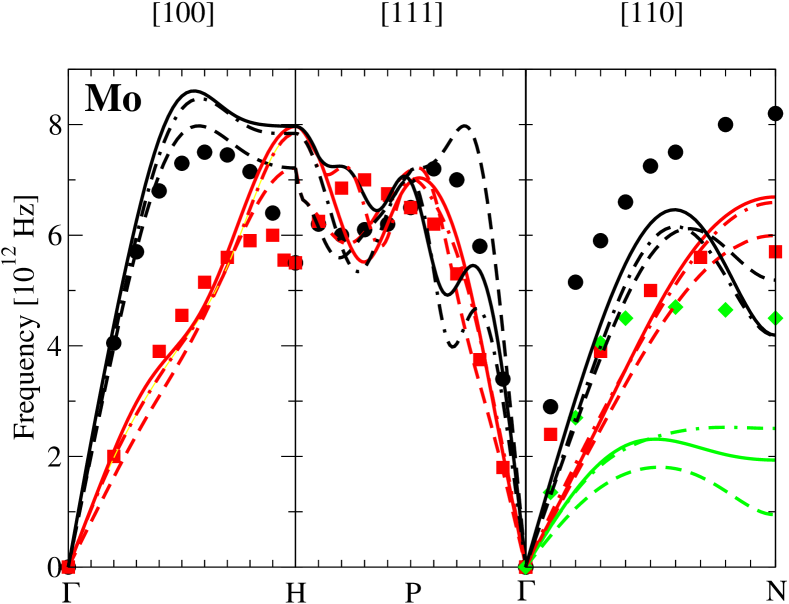
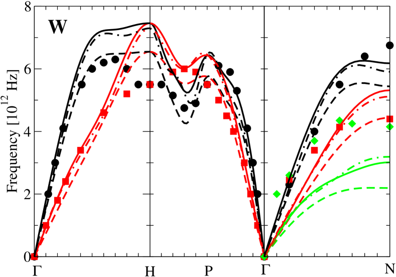
Figure 9: Phonon dispersion curves. Symbols represent experimental data Powell et al. (1968); Chen and Brockhouse (1964), full lines the analytic BOP, dashed lines the numerical BOP and dot-and-dash lines TB. Black, red and green represent longitudinal, transversal (T1) and transversal (T2) vibration modes, respectively.

The Cartesian coordinates in reciprocal space of the high-symmetry points are: $\Gamma$=(0, 0, 0), H=(0, 1, 0), N=(0.5, 0.5, 0) and P=(0.5, 0.5, 0.5) in units of 2$\pi/a_{0}$, where $a_{0}$ is the lattice parameter. We find good overall agreement of the TB and BOP calculations with the experimental data. The most considerable deviation is the transversal T2 mode that is too soft in both Mo and W. This deviation can be reduced by introducing screened bond-integrals to the TB model Mrovec et al. (2004). Comparing the BOP results, we find that the analytic BOP follows the TB results more closely than the numerical BOP. The difference between analytic and numerical BOP can be tracked down to the difference in forces on atoms that are used to construct the force constant matrices in the small displacement approach that we used to determine the phonon dispersion curves.

IV Conclusions

We present a detailed comparison of numerical and analytic bond-order potentials (BOP) based on established BOP parametrisations for the bcc refractory metals Mo and W. We find that both BOP formalisms capture the electronic density of states in good agreement with TB, in line with previous works. We also find good overall agreement of numerical and analytic BOP for the calculation of binding energies, aside from small deviations due to the numerical integration scheme in the numerical BOP. Despite the good agreement for the bcc ground-state properties, for the sequence of structural stability and for crystallographic transformation-paths, we find that the binding energies calculated with analytic BOP tend to agree slightly better with the TB results than the numerical BOP. The situation is different in our comparison for point defects and phonon spectra, i.e. for situations where atomic forces play an important role. While the forces in the analytic BOP formalism are strictly consistent with the derivative of the binding energy, this is not true for the numerical BOPs. For this reason we find that the analytic BOPs provide a better agreement with the TB results for point defects and phonon spectra than the numerical BOPs.