Computational design of nanophotonic structures using an adaptive finite element method

Abstract

We consider the problem of the construction of the nanophotonic structures of arbitrary geometry with prescribed desired properties. We reformulate this problem as an optimization problem for the Tikhonov functional which is minimized on adaptively locally refined meshes. These meshes are refined only in places where the nanophotonic structure should be designed. Our special symmetric mesh refinement procedure allows the construction of different nanophotonic structures. We illustrate efficiency of our adaptive optimization algorithm on the construction of nanophotonic structure in two dimensions.

1 Introduction

The goal of this work is to develop a new optimization algorithm that can construct arbitrary nanophotonic structures from desired scattering parameters. Nanophotonics is the study of the interaction of electromagnetic waves with structures that have feature sizes equal or smaller than the wavelength of the waves. Examples are photonic crystals (structured on the wavelength scale), metamaterials (subwavelength structured media with new optical properties that are not available from natural materials) and plasmonic devices (exploiting collective excitations in metals that result in strong field enhancement) [18, 20, 21, 26].

In this paper, we present a nonparametric optimization algorithm that can find inner structure of the domain with arbitrary geometry. To do that we apply an adaptive finite element method of [2, 7] with iterative choice of the regularization parameter [1]. We illustrate the efficiency of the proposed adaptive optimization method on the solution of the hyperbolic coefficient inverse problem (CIP) in two dimensions. The goal of our numerical simulations is to reconstruct the permittivity function of the hyperbolic equation from single observations of the transmitted and backscattered solution of this equation in space and time. For computational solution of this inverse problem we use the domain decomposition method of [3]. To solve our CIP we minimize the corresponding Tikhonov functional via Lagrangian approach. This approach is similar to the one applied recently in [2, 6, 7, 8, 9] for the solution of different hyperbolic CIPs: we find optimality conditions which express stationarity of the Lagrangian, involving the solution of state and adjoint equations together with an equation expressing that the gradient of the Lagrangian with respect to the permittivity function vanishes. Then we construct an adaptive conjugate gradient algorithm and compute the unknown permittivity function in an iterative process by solving in every step the state and adjoint hyperbolic equations and updating in this way the desired permittivity function.

2 Statement of the forward and inverse problems

Let $x=(x_{1},x_{2})$ denotes a point in $\mathbb{R}^{2}$ in an unbounded domain $D$. In this work we consider the propagation of electromagnetic waves in two dimensions with a field polarization. Thus, we model the wave propagation by the following Cauchy problem for the scalar wave equation:

(1) $$\begin{cases}\varepsilon(x)\frac{\partial^{2}E}{\partial t^{2}}-\triangle E=\delta(x_{2}-x_{0})p(t)&~{}\mbox{in}~{}~{}\mathbb{R}^{2}\times(0,\infty),\\ E(x,0)=f_{0}(x),~{}~{}~{}E_{t}(x,0)=0&~{}\mbox{in}~{}~{}D.\end{cases}$$

Here, $E$ is the electric field generated by the plane wave $p(t)$ which is incident at $x_{2}=x_{0}$ and propagates along $x_{2}$ axis, $\varepsilon(x)$ is the spatially distributed dielectric permittivity. We note that in this work we use the single equation (1) instead of the full Maxwell’s equations, since in [4] was demonstrated numerically that in the similar numerical setting, as we will use in this note, other components of the electric field are negligible compared to the initialized one. We also note that a scalar model of the wave equation was used successfully to validate reconstruction of the dielectric permittivity function with transmitted [10, 11] and backscattered experimental data [12, 13, 19, 22, 23].

Let now $D\subset\mathbb{R}^{2}$ be a convex bounded domain with the boundary $\partial D\in C^{2}$. We denote by $D_{T}:=D\times(0,T),\partial D_{T}:=\partial D\times(0,T),T>0$ and assume that

(2) $$f_{0}\in H^{1}(D),\varepsilon(x)\in C^{2}(D).$$

For computational solution of (1) we use the domain decomposition finite element/finite difference (FE/FD) method of [3, 5] which was applied for the solution of different coefficient inverse problems for the acoustic wave equation in [2, 3, 7]. To apply method of [3, 5] we decompose $D$ into two regions $D_{FEM}$ and $D_{FDM}$ such that the whole domain $D=D_{FEM}\cup D_{FDM}$, and $D_{FEM}\cap D_{FDM}=\emptyset$. In $D_{FEM}$ we use the finite element method (FEM), and in $D_{FDM}$ we will use the Finite Difference Method (FDM). We avoid instabilities at interfaces between FE and FD domains since FE and FD discretization schemes coincide on two common structured layers with $\varepsilon(x)=1$ in them.

Let the boundary $\partial D$ be such that $\partial D=\partial_{1}D\cup\partial_{2}D\cup\partial_{3}D$ where $\partial_{1}D$ and $\partial_{2}D$ are, respectively, front and back sides of the domain $D$, and $\partial_{3}D$ is the union of left, right, top and bottom sides of this domain. At $S_{T_{1}}:=\partial_{1}D\times(0,T)$ and $S_{T_{2}}:=\partial_{2}D\times(0,T)$ we have time-dependent backscattering and transmission observations, correspondingly. We define $S_{1,1}:=\partial_{1}D\times(0,t_{1}]$, $S_{1,2}:=\partial_{1}D\times(t_{1},T)$, and $S_{3}:=\partial_{3}D\times(0,T)$. We also introduce the following spaces of real valued functions

(3) $$\begin{split}H_{E}^{1}(D_{T})&:=\{w\in H^{1}(D_{T}):w(\cdot,0)=0\},\\ H_{\lambda}^{1}(D_{T})&:=\{w\in H^{1}(D_{T}):w(\cdot,T)=0\},\\ U^{1}&=H_{E}^{1}(D_{T})\times H_{\lambda}^{1}(D_{T})\times C\left(\overline{D}\right),\\ \end{split}$$

and define standard $L_{2}$ inner product and space-time norms, correspondingly, as

$$\begin{split}((u,v))_{D_{T}}&=\int_{D}\int_{0}^{T}uv~{}dxdt,~{}\|u\|_{L_{2}(D_{T})}^{2}=((u,u))_{D_{T}},\\ (u,v)_{D}&=\int_{D}uv~{}dx,~{}\|u\|_{L_{2}(D)}^{2}=(u,u)_{D}.\end{split}$$

In our computations we have used the following model problem

(4) $$\begin{cases}\varepsilon\frac{\partial^{2}E}{\partial t^{2}}-\triangle E=0&~{}\mbox{in}~{}~{}D_{T},\\ E(x,0)=f_{0}(x),~{}~{}~{}E_{t}(x,0)=0&~{}\mbox{in}~{}~{}D,\\ \partial_{n}E=p\left(t\right)&~{}\mbox{on}~{}S_{1,1},\\ \partial_{n}E=-\partial_{t}E&~{}\mbox{on}~{}S_{1,2},\\ \partial_{n}E=-\partial_{t}E&~{}\mbox{on}~{}S_{T_{2}},\\ \partial_{n}E=0&~{}\mbox{on}~{}S_{3}.\\ \end{cases}$$

In (1) we use the first order absorbing boundary conditions [16]. These conditions are exact in the case of computations of section 6 since we initialize the plane wave orthogonal to the domain of propagation.

We choose the coefficient $\varepsilon(x)$ in (1) such that

(5) $$\begin{cases}\varepsilon\left(x\right)\in\left(0,M\right],M=const.>0,&\text{ for }x\in D_{FEM},\\ \varepsilon(x)=1&\text{ for }x\in D_{FDM}.\end{cases}$$

We consider the following inverse problem

Inverse Problem (IP)

Let the coefficient $\varepsilon\left(x\right)$ in the problem (4) satisfy conditions (5) and assume that $\varepsilon\left(x\right)$ is unknown in the domain $D\diagdown D_{FDM}$. Determine the function $\varepsilon\left(x\right)$  in (4) for $x\in D\diagdown D_{FDM},$  assuming that the following function $\widetilde{E}\left(x,t\right)$ is known

(6) $$E\left(x,t\right)=\widetilde{E}\left(x,t\right),~{}\forall\left(x,t\right)\in S_{T_{1}}\cup S_{T_{2}}.$$

3 Optimization method

In this section we present the reconstruction method to solve inverse problem IP. This method is based on the finding of the stationary point of the following Tikhonov functional

(7) $$F(E,\varepsilon)=\frac{1}{2}\int_{S_{T_{1}}\cup S_{T_{2}}}(E-\widetilde{E})^{2}z_{\delta}(t)d\sigma dt+\frac{1}{2}\gamma\int_{D}(\varepsilon-\varepsilon_{g})^{2}~{}~{}dx,$$

where $E$ satisfies the equations (4), $\varepsilon_{0}$ is the initial guess for $\varepsilon$, $\widetilde{E}$ is the observed field at $S_{T_{1}}\cup S_{T_{2}}$, $\gamma>0$ is the regularization parameter and $z_{\delta}$ can be chosen as in [8].

To find minimum of (7) we use the Lagrangian approach [2, 7] and define the following Lagrangian

(8) $$\begin{split}L(v)&=F(E,\varepsilon)-\int_{D_{T}}\varepsilon\frac{\partial\lambda}{\partial t}\frac{\partial E}{\partial t}~{}dxdt+\int_{D_{T}}(\nabla E)(\nabla\lambda)~{}dxdt\\ &-\int_{S_{1,1}}\lambda p(t)~{}d\sigma dt+\int_{S_{1,2}}\lambda\partial_{t}E~{}d\sigma dt+\int_{S_{T_{2}}}\lambda\partial_{t}E~{}d\sigma dt,\\ \end{split}$$

where $v=(E,\lambda,\varepsilon)\in U^{1}$, and search for a stationary point with respect to $v$ satisfying $\forall\bar{v}=(\bar{E},\bar{\lambda},\bar{\varepsilon})\in U^{1}$

(9) $$L^{\prime}(v;\bar{v})=0,$$

where $L^{\prime}(v;\cdot)$ is the Jacobian of $L$ at $v$.

Similarly with [2, 7] we use conditions $\lambda\left(x,T\right)=\partial_{t}\lambda\left(x,T\right)=0$ and imply such conditions on the function $\lambda$ that $L\left(E,\lambda,\varepsilon\right):=L\left(v\right)=F\left(E,\varepsilon\right).$ We also use conditions (5) on $\partial D$, together with initial and boundary conditions of (4) to get that for all $\bar{v}\in U^{1}$,

(10) $$\begin{split}0&=\frac{\partial L}{\partial\lambda}(v)(\bar{\lambda})=-\int_{D_{T}}\varepsilon\frac{\partial\bar{\lambda}}{\partial t}\frac{\partial E}{\partial t}~{}dxdt+\int_{D_{T}}(\nabla E)(\nabla\bar{\lambda})~{}dxdt\\ &-\int_{S_{1,1}}\bar{\lambda}p(t)~{}d\sigma dt+\int_{S_{1,2}}\bar{\lambda}\partial_{t}E~{}d\sigma dt+\int_{S_{T_{2}}}\bar{\lambda}\partial_{t}E~{}d\sigma dt,~{}~{}\forall\bar{\lambda}\in H_{\lambda}^{1}(D_{T}),\end{split}$$

(11) $$\begin{split}0&=\frac{\partial L}{\partial E}(v)(\bar{E})=\int_{S_{T}}(E-\widetilde{E})~{}\bar{E}~{}z_{\delta}~{}d\sigma dt-\int_{D}\varepsilon\frac{\partial{\lambda}}{\partial t}(x,0)\bar{E}(x,0)~{}dx-\int_{S_{1,2}\cup S_{T_{2}}}\frac{\partial{\lambda}}{\partial t}\bar{E}~{}d\sigma dt\\ &-\int_{D_{T}}\varepsilon\frac{\partial\lambda}{\partial t}\frac{\partial\bar{E}}{\partial t}~{}dxdt+\int_{D_{T}}(\nabla\lambda)(\nabla\bar{E})~{}dxdt,~{}\forall\bar{E}\in H_{E}^{1}(D_{T}),\end{split}$$

(12) $$0=\frac{\partial L}{\partial\varepsilon}(v)(\bar{\varepsilon})=-\int_{D_{T}}\frac{\partial\lambda}{\partial t}\frac{\partial E}{\partial t}\bar{\varepsilon}~{}dxdt+\gamma\int_{D}(\varepsilon-\varepsilon_{g})\bar{\varepsilon}~{}dx,~{}x\in D.$$

We observe that (10) is the weak formulation of the state equation (4) and (11) is the weak formulation of the following adjoint problem

(13) $$\begin{cases}\varepsilon\frac{\partial^{2}\lambda}{\partial t^{2}}-\triangle\lambda=-(E-\widetilde{E})z_{\delta}&~{}x\in S_{T},\\ \lambda(\cdot,T)=\frac{\partial\lambda}{\partial t}(\cdot,T)=0,\\ \partial_{n}\lambda=\partial_{t}\lambda&~{}\mbox{on}~{}S_{1,2},\\ \partial_{n}\lambda=\partial_{t}\lambda&~{}\mbox{on}~{}S_{T_{2}},\\ \partial_{n}\lambda=0&~{}\mbox{on}~{}S_{3}.\end{cases}$$

4 Discretization of the domain decomposition FE/FD method

As was mentioned above for the numerical solution of (1) we use the domain decomposition FE/FD method of [3, 5]. Similarly with these works, in our computations we decompose the finite difference domain $D_{FDM}$ into squares and the finite element domain $D_{FDM}$ - into triangles. For FDM discretization we use the standard difference discretization of the equation (4) and obtain an explicit scheme as in [3].

For the finite element discretization of $D_{FEM}$ we define a partition $K_{h}=\{K\}$ which consists of triangles. We define by $h$ the mesh function as $h|_{K}=h_{K}$, where $h_{K}$ is the local diameter of the element $K$, and assume the minimal angle condition on the $K_{h}$ [14]. Let $J_{\tau}=\left\{J\right\}$ be a partition of the time interval $(0,\,T)$ into subintervals $J=(t_{k-1},\,t_{k}]$ of uniform length $\tau=t_{k}-t_{k-1}$.

To solve the state problem (4) and the adjoint problem (13) we define the finite element spaces, $W_{h}^{E}\subset H_{E}^{1}\left(D_{T}\right)$ and $W_{h}^{\lambda}\subset H_{\lambda}^{1}\left(D_{T}\right)$. First, we introduce the finite element trial space $W_{h}^{u}$

(14) $$W_{h}^{u}:=\{w\in H_{u}^{1}(D_{T}):w|_{K\times J}\in P_{1}(K)\times P_{1}(J),~{}\forall K\in K_{h},~{}\forall J\in J_{\tau}\},$$

where $P_{1}(K)$ and $P_{1}(J)$ denote the set of linear functions on $K$ and $J$, respectively. We also introduce the finite element test space $W_{h}^{\lambda}$ as

(15) $$W_{h}^{\lambda}:=\{w\in H_{\lambda}^{1}(D_{T}):w|_{K\times J}\in P_{1}(K)\times P_{1}(J),~{}\forall K\in K_{h},~{}\forall J\in J_{\tau}\}.$$

To approximate the function $\varepsilon_{\mathrm{r}}$, we use the space of piecewise constant functions $C_{h}\subset L_{2}\left(D\right)$,

(16) $$C_{h}:=\{u\in L_{2}(D):u|_{K}\in P_{0}(K),~{}\forall K\in K_{h}\},$$

where $P_{0}(K)$ is the set of constant functions on $K$.

Setting $U_{h}=W_{h}^{E}\times W_{h}^{\lambda}\times C_{h}$, the finite element method for (9) now reads: Find $u_{h}\in U_{h}$, such that

(17) $$L^{\prime}(E_{h})(\bar{E})=0,~{}\forall\bar{E}\in U_{h}.$$

5 Adaptive conjugate gradient algorithm

To compute the minimum of the functional (7) we use the adaptive conjugate gradient method (ACGM). The regularization parameter $\gamma$ in ACGM is computed iteratively via rules of [1]. For the local mesh refinement we use a posteriori error estimate of [2, 7] which means that the finite element mesh in $D_{FEM}$ should be locally refined where the maximum norm of the Fréchet derivative of the Lagrangian with respect to the coefficient is large.

We denote

(18) $$\begin{split}{g}^{m}(x)=-{\int_{0}}^{T}\frac{\partial\lambda_{h}^{m}}{\partial t}\frac{\partial E_{h}^{m}}{\partial t}~{}dt+\gamma^{m}(\varepsilon_{h}^{m}-\varepsilon_{g}),\end{split}$$

where $\varepsilon_{h}^{m}$ is approximation of the function $\varepsilon_{h}$ on the iteration $m$, $E_{h}\left(x,t,\varepsilon_{h}^{m}\right),\lambda_{h}\left(x,t,\varepsilon_{h}^{m}\right)$ are computed by solving the state (4) and adjoint (13) problems, respectively, with $\varepsilon:=\varepsilon_{h}^{m}$.

Algorithm

• Step 0. Choose initial mesh $K_{h}$ in $D_{FEM}$ and time partition $J_{\tau}$ of the time interval $\left(0,T\right)$ as described in section 4. Start with the initial approximation $\varepsilon_{h}^{0}=\varepsilon_{g}$ and compute the sequences of $\varepsilon_{h}^{m}$ via the following steps:

• Step 1. Compute solutions $E_{h}\left(x,t,\varepsilon_{h}^{m}\right)$ and $\lambda_{h}\left(x,t,\varepsilon_{h}^{m}\right)$ of state (4) and adjoint (13) problems on $K_{h}$ and $J_{\tau}$.

• Step 2. Update the coefficient $\varepsilon_{h}:=\varepsilon_{h}^{m+1}$ on $K_{h}$ and $J_{\tau}$ using the conjugate gradient method

  (19) $$\begin{split}\varepsilon_{h}^{m+1}&=\varepsilon_{h}^{m}+\alpha^{m}d^{m}(x),\end{split}$$

  where

  $$\begin{split}d^{m}(x)&=-g^{m}(x)+\beta^{m}d^{m-1}(x),\end{split}$$

  with

  $$\begin{split}\beta^{m}&=\frac{\|g^{m}(x)\|^{2}}{\|g^{m-1}(x)\|^{2}},\end{split}$$

  where $d^{0}(x)=-g^{0}(x)$. In (19) the step size $\alpha$ in the gradient update is computed as

  (20) $$\alpha^{m}=-\frac{((g^{m},d^{m}))}{\gamma^{m}{\left\lVert{\textstyle d^{m}}\right\rVert}^{2}},$$

  and the regularization parameter $\gamma$ is computed iteratively accordingly to [1] as

  (21) $$\gamma^{m}=\frac{\gamma_{0}}{(m+1)^{p}},p\in(0,1).$$

• Step 3. Stop computing $\varepsilon_{h}^{m}$ and obtain the function $\varepsilon_{h}$ at $M=m$ if either $\|g^{m}\|_{L_{2}(D_{FEM})}\leq\theta$ or norms $\|g^{m}\|_{L_{2}(D_{FEM})}$ are stabilized. Here $\theta$ is the tolerance in updates $m$ of gradient method. Otherwise set $m:=m+1$ and go to step 1.

• Step 4. Refine the mesh $K_{h}$ where

  (22) $$|g^{M}(x)|\geq C\max_{x\in{D}_{FEM}}|g^{M}(x)|,$$

  where the constant $C\in\left(0,\,1\right)$ is chosen by the user.

• Step 5. Construct a new mesh $K_{h}$ in $D_{FEM}$ and a new partition $J_{\tau}$ of the time interval $\left(0,\,T\right)$. On $J_{\tau}$ the new time step $\tau$ should be chosen in such a way that the CFL condition is satisfied.

• Step 6. Interpolate the initial approximation $\varepsilon_{g}$ from the previous space mesh to the new one. Set $m=1$ and return to step 1.

• Step 7. Stop refinements of $K_{h}$ if norms defined in step 3 either increase or stabilize, compared with the previous space mesh.

Remark

In our computations at step 4 of the adaptive algorithm we refine only a such domain of $D_{FEM}$ which should be designed since we assume that we know in advance the dielectric permittivity in all other parts of $D_{FEM}$.

6 Numerical Studies

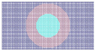
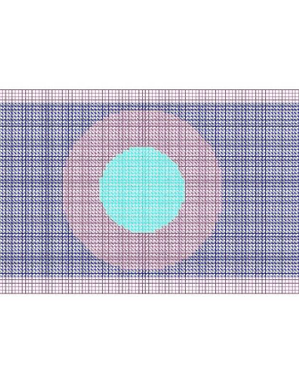
The goal of this section is to present possibility of the computational design of nanophotonic structures with some prescribed property. We have chosen to design a structure which have a property to generate a small reflections as possible. This problem is equivalent to IP. Thus, we will reconstruct a function $\varepsilon(x)$ inside a domain $D_{FEM}$ using the ACGM algorithm of section 5. We assume, that this function is known inside $D_{FDM}$ and is set to be $\varepsilon(x)=1$. Moreover, we decompose also the domain $\mathbf{D}_{FEM}$ into three different domains $D_{1},D_{2},D_{3}$ such that $\mathbf{D}_{FEM}=D_{1}\cup D_{2}\cup D_{3}$ which are intersecting only by their boundaries, see Figure 1. The boundary of $D_{FEM}$ we define as $\partial D_{FEM}$, and the boundary of $D_{1}$ we define as $\partial D_{1}$. The goal of our numerical tests is to reconstruct the dielectric permittivity function of the approximately cyclic domain $D_{2}$ of Figure 1 which produce a small reflections as possible.

In our studies we initialize a plane wave $p(t)$ as the boundary condition on $S_{T_{1}}$, see (23). Initial conditions in (4) are set to be zero. In all computations we used the domain decomposition method of [3] implemented in the software package WavES [25]. Our computational geometry $D$ is split into two geometries $D_{FEM}$ and $D_{FDM}$ as described in section 2, such that $D=D_{FEM}\cup D_{FDM}$, see Figure 1. We set the dimensionless computational domain $D$ as

$$D=\left\{x=(x_{1},x_{2})\in(-1.1,1.1)\times(-0.62,0.62)\right\},$$

and the domain $D_{FEM}$ as

$$D_{FEM}=\left\{x=(x_{1},x_{2})\in((-1.0,1.0)\times(-0.52,0.52)\right\}.$$

The space mesh in $D_{FEM}$ and in $D_{FDM}$ consists of triangles and squares, respectively. We choose the initial mesh size $h=0.02$ in $D=D_{FEM}\cup D_{FDM}$, as well as in the overlapping regions between FE/FD domains.

We initialize a plane wave $f(t)$ in the equation (4) in $D$ in time $T=[0,2.0]$ such that

(23) $$\begin{split}f\left(t\right)=\left\{\begin{array}[]{ll}\sin\left(\omega t\right),&\text{ if }t\in\left(0,\frac{2\pi}{\omega}\right),\\ 0,&\text{ if }t>\frac{2\pi}{\omega}.\end{array}\right.\end{split}$$

As the forward problem in $D_{FDM}$ we solve the problem (4) choosing $\varepsilon=1$ and $D=D_{FDM}$, and in $D_{FEM}$ we solve

(24) $$\begin{split}\varepsilon\frac{\partial^{2}E}{\partial t^{2}}-\triangle E&=0,~{}\mbox{in}~{}~{}D_{{FEM}},\\ E(x,0)=0,~{}~{}~{}E_{t}(x,0)&=0~{}\mbox{in}~{}~{}D_{FEM},\\ E(x,t)|_{\partial D_{FEM}}&=E(x,t)|_{\partial D_{{FDM}_{I}}},\\ \partial_{n}E&=0~{}\mbox{on}~{}~{}\partial D_{1}.\end{split}$$

Here, $\partial D_{{FDM}_{I}}$ denote structured nodes of $D_{FDM}$ which have the same coordinates as nodes at $\partial D_{FEM}$, see details in [3]. We note, that we use the boundary condition $\partial_{n}E=0$ on $\partial D_{1}$ which says that waves are not penetrated into $D_{1}$.

We also note that in $D_{FDM}$ the adjoint problem will be the following wave equation with $\varepsilon=1$ in $D_{FDM}$:

(25) $$\begin{split}\frac{\partial^{2}\lambda}{\partial t^{2}}-\triangle\lambda&=-(E-\tilde{E})z_{\delta},~{}\mbox{in}~{}~{}S_{T_{1}}\cup S_{T_{2}},\\ \lambda(x,T)=0,~{}~{}~{}\lambda_{t}(x,T)&=0~{}\mbox{in}~{}~{}D,\\ \partial_{n}\lambda(x,t)&=0~{}\mbox{on}~{}S_{3}.\end{split}$$

Thus, as the adjoint problem in $D_{FDM}$ we solve the problem (25) and in $D_{FEM}$ we have to solve

(26) $$\begin{split}\varepsilon\frac{\partial^{2}\lambda}{\partial t^{2}}-\triangle\lambda&=0,~{}\mbox{in}~{}~{}D_{{FEM}},\\ \lambda(x,T)=0,~{}~{}~{}\lambda_{t}(x,T)&=0~{}\mbox{in}~{}~{}D_{FEM},\\ \lambda(x,t)|_{\partial D_{FEM}}&=\lambda(x,t)|_{\partial D_{{FDM}_{II}}},\\ \partial_{n}\lambda&=0,~{}\mbox{on}~{}~{}\partial D_{1}.\end{split}$$

Here, $\partial D_{{FDM}_{II}}$ denote the inner boundary of $D_{FDM}$, see details in [3].

As initial guess $\varepsilon_{g}(x)$ we take different constant values of the function $\varepsilon(x)$ inside domain of $D_{2}$ of Figure 1 on the coarse non-refined mesh, and we take $\varepsilon(x)=1.0$ everywhere else in $D$. We choose three different constant values of $\varepsilon_{g}(x)=\{0.5,1.5,2.0,2.5\}$ inside $D_{2}$. We define that the minimal and maximal values of the function $\varepsilon(x)$ belongs to the following set $M_{\varepsilon}$ of admissible parameters

(27) $$\begin{split}M_{\varepsilon}\in\left\{\varepsilon\in C(\overline{D})|\frac{1}{\max_{D_{2}}\varepsilon_{g}(x)}\leq\varepsilon(x)\leq\max_{D_{2}}\varepsilon_{g}(x)\right\}.\end{split}$$

The time step is chosen to be $\tau=0.002$ which satisfies the CFL condition [27].

6.1 Reconstructions

We generate data at the observation points at $S_{T_{1}}\cup S_{T_{2}}$ by solving the forward problem (4) in the time interval $t=[0,2.0]$, with function $f(t)$ given by (23) and $\omega=40$. To generate $\tilde{E}$ at $S_{T_{1}}\cup S_{T_{2}}$ we take the function $\varepsilon(x)=1$ for all $x$ in $D$ and solve the problem (4) with a plane wave (23) and $\omega=40$.

We regularize the solution of the inverse problem by starting computations with regularization parameter $\gamma=0.01$ in (7) and then updating this parameter iteratively in ACGM by formula (21). Computing of the regularization parameter by this way is optimal one for our problem. We refer to [17] for different techniques for choice of a regularization parameters.

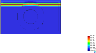
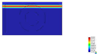
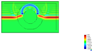
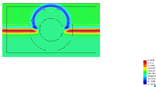
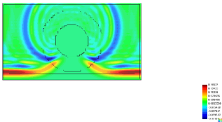
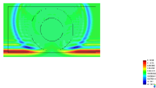
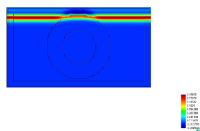
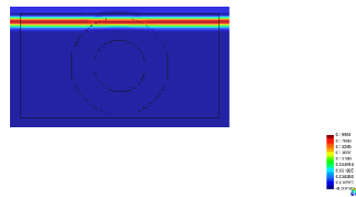
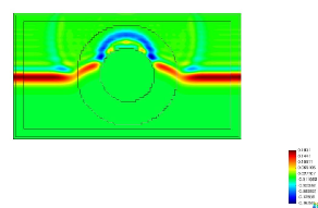
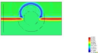
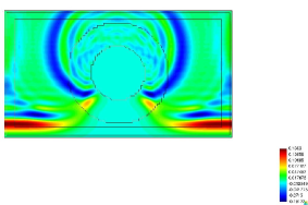
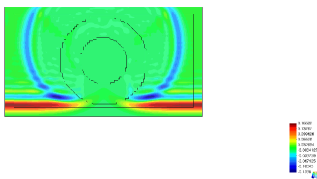
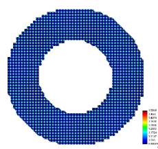
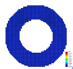
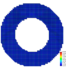
Figures 3, 4 show time-dependent reflections from the dielectric permittivity function when $\varepsilon=\varepsilon_{g}$ (on the left) and after optimization procedure after four refinements of the mesh in $D_{2}$ (on the right). All right figures of Figures 3, 4 show significant reduction of reflections compared with left figures.

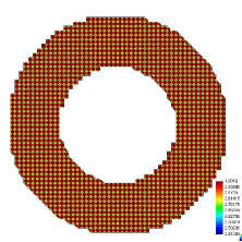
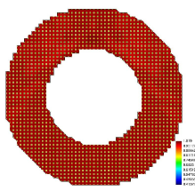
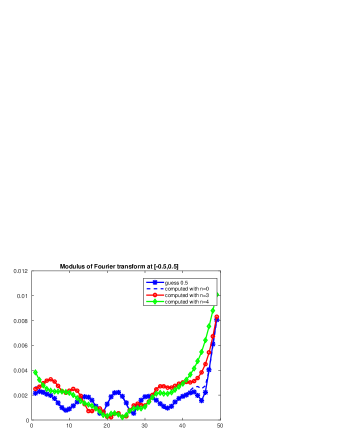
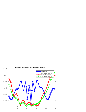
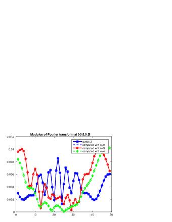
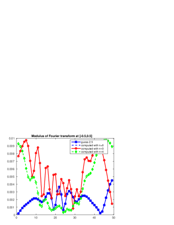
Figures 5 present reconstructions which we have obtained on three and four times adaptively refined mesh when we take different initial guesses on the coarse mesh. All guesses produce different structures of the domain $D_{2}$ with different values of the function $\varepsilon(x)$ inside it. Smallest reflections we obtain taking the initial guess $\varepsilon_{g}=0.5$ inside $D_{2}$, and largest - with $\varepsilon_{g}=2.5$, see Figure 6. Figures 6 present comparison of reflections from initial and optimized functions $\varepsilon(x)$ after applying the Fourier transform to the solution $E(x,t)$.

Interesting designed domains are obtained with initial guesses $\varepsilon_{g}(x)=\{0.5,1.5,2.0\}$. In this case we obtain optimized values of $\varepsilon(x)$ which can be of physical interest, see Figures 5-b), d), f).

a) $D$

b) $D_{FEM}$

Figure 1: Computational coarse FE/FD mesh used in the domain decomposition in $D$. b) The finite element mesh in $D_{FEM}$.

a) $n=3$

b) $n=4$

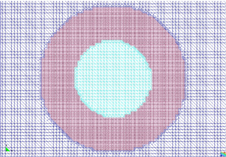
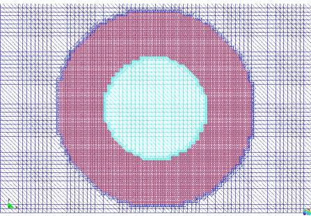
Figure 2: Zoomed main parts of computationally adaptively refined meshes for $\varepsilon_{g}=1.5$: a) three-times refined mesh; b) four-times refined mesh.

a) t= 0.3	b) t= 0.3
c) t= 0.78	d) t= 0.78
e) t= 1.26	f) t= 1.26

Figure 3: Computational solution of (4) using domain decomposition method of [3] at different times: a),c),e) on the coarse mesh with $\varepsilon_{g}=1.5$ in $D_{2}$; b),d),f) on the four times refined mesh with optimized $\varepsilon$ of Figure 5-d).

a) t= 0.3	b) t= 0.3
c) t= 0.78	d) t= 0.78
e) t= 1.26	f) t= 1.26

Figure 4: Computational solution of (4) using domain decomposition method of [3] at different times: a),c),e) on the coarse mesh with $\varepsilon_{g}=2$ in $D_{2}$; b),d),f) on the four times refined mesh with optimized $\varepsilon$ of Figure 5-f).

a) $\varepsilon_{g}=0.5,n=3$	b) $\varepsilon_{g}=0.5,n=4$
c) $\varepsilon_{g}=1.5,n=3$	d) $\varepsilon_{g}=1.5,n=4$
e) $\varepsilon_{g}=2,n=3$	f) $\varepsilon_{g}=2.0,n=4$

Figure 5: Reconstructions in $D_{2}$ on three and four-times adaptively refined meshes for different $\varepsilon_{g}$.

a) $\varepsilon_{g}=0.5$	b) $\varepsilon_{g}=1.5$
c) $\varepsilon_{g}=2.0$	d) $\varepsilon_{g}=2.5$

Figure 6: Modulus of the Fourier transform at $\partial_{2}D$ for different $\varepsilon_{g}$ in $D_{2}$ after applying the ACGM algorithm. Here, $n$ is the number of refinements of the mesh.

References

• [1] Bakushinsky A., Kokurin M.Y., Smirnova A., Iterative Methods for Ill-posed Problems, Inverse and Ill-Posed Problems Series 54, De Gruyter, 2011.
• [2] L. Beilina, Adaptive hybrid FEM/FDM methods for inverse scattering problems. Inverse Problems and Information Technologies, V.1, N.3, 73-116, 2002.
• [3] L. Beilina, Domain decomposition finite element/finite difference method for the conductivity reconstruction in a hyperbolic equation, Communications in Nonlinear Science and Numerical Simulation, Elsevier, 37, p.222-237, 2016.
• [4] L. Beilina, Energy estimates and numerical verification of the stabilized domain decomposition finite element/finite difference approach for time-dependent Maxwell’s system, Cent. Eur. J. Math., 11, 702-733, 2013.
• [5] L. Beilina, K. Samuelsson and K. Åhlander, Efficiency of a hybrid method for the wave equation. Proceedings of the International Conference on Finite Element Methods: Three Dimensional Problems. GAKUTO International Series, Mathematical Sciences and Applications, V. 15, 2001.
• [6] L. Beilina, Adaptive hybrid finite element/difference method for Maxwell’s equations: an a priory error estimate and efficiency, Applied and Computational Mathematics (ACM), 9 (2), 176-197, 2010.
• [7] L. Beilina and C. Johnson, A posteriori error estimation in computational inverse scattering, Mathematical Models in Applied Sciences, 1, 23-35, 2005.
• [8] L. Beilina, M. Cristofol and K. Niinimäki, Optimization approach for the simultaneous reconstruction of the dielectric permittivity and magnetic permeability functions from limited observations, Inverse Problems and Imaging, 9 (1), pp. 1-25, 2015.
• [9] L. Beilina and K. Niinimäki, Numerical studies of the Lagrangian approach for reconstruction of the conductivity in a waveguide, arXiv:1510.00499, 2015.
• [10] L. Beilina and M. V. Klibanov, Reconstruction of dielectrics from experimental data via a hybrid globally convergent/adaptive inverse algorithm, Inverse Problems, 26, 125009, 2010.
• [11] L. Beilina and M. V. Klibanov, Relaxation property for the adaptivity for ill-posed problems, Appl. Anal., 93, pp. 223–253., 2014.
• [12] L. Beilina, Nguyen T.T., M. Klibanov, and J. Malmberg, Reconstruction of shapes and refractive indices from backscattering experimental data using the adaptivity, Inverse Problems 30, 105007 2014.
• [13] L. Beilina, Nguyen T.T., M. Klibanov, and J. Malmberg, Globally convergent and adaptive finite element methods in imaging of buried objects from experimental backscattering radar measurements,J. Comput. Appl. Math., 289, pp. 371-301, 2015, doi:10.1016/j.cam.2014.11.055.
• [14] S. C. Brenner and L. R. Scott, The Mathematical Theory of Finite Element Methods, Springer-Verlag, Berlin, 1994.
• [15] G. C. Cohen, Higher Order Numerical Methods for Transient Wave Equations, Springer-Verlag, Berlin, 2002.
• [16] B. Engquist and A. Majda, Absorbing boundary conditions for the numerical simulation of waves,  Math. Comp., 31, 629-651, 1977.
• [17] H. W. Engl, M. Hanke and A. Neubauer,  Regularization of Inverse Problems, Kluwer Academic Publishers, Boston, 2000.
• [18] Joannopoulos, Johnson, Winn and Meade, Photonic Crystals: Molding the Flow of Light, Second edition, Princeton Univ. Press, 2008.
• [19] Kuzhuget, A.V., Beilina, L., Klibanov, M.V., Sullivan, A., Nguyen, L., Fiddy, M.A., Blind experimental data collected in the field and an approximately globally convergent inverse algorithm, Inverse Problems, V.28, N.9, 2012, DOI:10.1088/0266-5611/28/9/095007
• [20] Maier, Plasmonics: Fundamentals and Applications, Springer, 2007.
• [21] Soukoulis, Wegener, Nature Photon. 5, 523, 2011.
• [22] N. T. Thành, L. Beilina, M. V. Klibanov and M. A. Fiddy, Reconstruction of the refractive index from experimental backscattering data using a globally convergent inverse method, SIAM J. Scientific Computing, 36 (3), pp.273-293, 2014.
• [23] N. T. Thành, L. Beilina, M. V. Klibanov, M. A. Fiddy, Imaging of buried objects from experimental backscattering time-dependent measurements using a globally convergent inverse algorithm, SIAM Journal on Imaging Sciences, 8(1), 757-786, 2015.
• [24] A. N. Tikhonov, A. V. Goncharsky, V. V. Stepanov and A. G. Yagola, Numerical Methods for the Solution of Ill-Posed Problems, Kluwer, London, 1995.
• [25] WavES, the software package, http://www.waves24.com .
• [26] Zheludev, Kivshar, Nature Mater. 11, 917, 2012.
• [27] R. Courant, K. Friedrichs and H. Lewy, On the partial differential equations od mathematical physics, IBM Journal of Research and Development, 11(2), 215-234, 1967.