Enhanced harmonic generation and wave-mixing via two-color multiphoton excitation of atoms/molecules

Abstract

We consider harmonics generation and wave-mixing by two-color multiphoton resonant excitation of three-level atoms/molecules in strong laser fields. The coherent part of the spectra corresponding to multicolor harmonics generation is investigated. The obtained analytical results on the basis of generalized rotating wave approximation are in a good agreement with numerical calculations. The results applied to the hydrogen atom and homonuclear diatomic molecular ion show that one can achieve efficient generation of moderately high multicolor harmonics via multiphoton resonant excitation by appropriate laser pulses.

I Introduction

Harmonics generation and wave-mixing are one of the basic phenomena of nonlinear optics which have been extensively studied both theoretically and experimentally with the advent of lasers NO . Recent advance in laser technologies has provided ultrahigh intensities for supershort laser pulses that makes achievable non-perturbative regime of harmonic generation, which significantly extends the spectral region accessible by lasers, in particular, for short wavelengths towards VUV/XUV or even X-ray radiation VUV ; XUV1 ; XUV2 ; XUV3 ; HGrev . Such short wavelength radiation is of great interest due to numerous significant applications, e.g. in quantum control, spectroscopy, sensing and imaging etc..

Depending on the laser-atom interaction parameters, harmonic generation may arise from bound-bound BB ; AAM2 ; AAM3 ; AAM1 ; Gib1 and bound-free-bound transitions via continuum spectrum Huillier ; BFB . Bound-bound mechanism of harmonic generation without ionization is more efficient for generation of moderately high harmonics AAM2 ; AAM3 . For this mechanism resonant interaction is of importance. Besides pure theoretical interest as a simple model, resonant interaction regime exhibits significant enhancement of frequency conversion efficiencies AAM2 ; AAM3 . However, to access highly excited states of atoms/molecules by optical lasers the multiphoton excitation problem arises. Required resonantly-driven multiphoton transition is effective for the systems with the mean dipole moments in the stationary states, or three-level atomic systems with close enough to each other two states and nonzero transition dipole moment between them AM . As a candidate, we have studied the hydrogenlike atomic and ionic systems where the atom has a mean dipole moment in the excited stationary states, because of accidental degeneracy for the orbital momentum AMP ; AAM4 . Other interesting examples of efficient direct multiphoton excitation are molecules with a permanent dipole moments Br1 , evenly charged molecular ions at large internuclear distances Gib2 , and artificial atoms Mer15 ; Oliver realized in circuit Quantum Electrodynamics (QED) setups CQED .

In the work AAM4 we have shown that the multiphoton resonant excitation of a three-level atomic/molecular system is efficient by the two bichromatic laser fields. Hence, having efficient two-color multiphoton resonant excitation scheme it is of interest to consider multicolor harmonic generation and wave-mixing processes by an atomic or molecular system under the such circumstances when only a bound states are involved in the interaction process, which is the purpose of the current paper. The presence of the second laser provides additional flexibility for the implementation of multiphoton resonance expanding the spectrum of possible combinations. Moreover, two-color excitation extends accessible scattering frequencies with sum- and difference components. In the current paper, we employ analytical approach for high-order multiphoton resonant excitation of quantum systems which has been previously developed by us AM ; AAM4 . Expression for the time-dependent mean dipole moment describing coherent part of scattering spectrum is obtained. The results based on this expression are applied to hydrogen atom and evenly charged homonuclear diatomic molecular ion. The main spectral characteristics of the considered process are in good agreement with the results of the performed numerical calculations. Estimations show that one can achieve enhanced generation of moderately high harmonics/wave-mixing via multiphoton resonant excitation by appropriate laser pulses. Our interest is also motivated by the advent of circuit QED setups CQED where one can realize artificial atoms of desired configuration. Thus, the obtained results may also be is of interest for artificial atoms, and the presented results can be scaled to other systems and diverse domains of the electromagnetic spectrum.

The paper is organized as follows. In section II, we present the analytical model and derive the coherent contribution to the multicolor harmonic spectra. In section III, we present some results of numerical calculations of the considered issue without a multiphoton resonant approximation and compare the obtained spectra with the analytical results. Here, we consider concrete systems, such as hydrogenlike atom and evenly charged molecular ion. Finally, conclusions are given in section IV.

II BASIC MODEL AND ANALYTICAL ANSATZ

We consider a three-level quantum system interacting with the two laser fields of frequencies $\omega_{1}$ and $\omega_{2}$ as shown in Fig.(1a). It is assumed that the system is in a $V$ configuration in which a pair of upper levels $\left|2\right\rangle$ and $\left|3\right\rangle$ with permanent dipole moments are coupled to a lower level $\left|1\right\rangle$. Another possible three-level scheme is $\Gamma$ configuration shown in Fig.(1b). In this case the lower level $\left|1\right\rangle$ is coupled to an upper level $\left|2\right\rangle$ which has a strong dipole coupling to an adjacent level $\left|3\right\rangle$. If the separation of the energy levels of the excited states is smaller than laser-atom interaction energy then by a unitary transformation AM the problem can be reduced to the $V$ configuration Fig.(1a). As an illustrative example may serve hydrogenlike atom considered in parabolic LL3 and more conventional spherical coordinates. In parabolic coordinates, the atom has a mean dipole moment in the excited states, while in the second case because of the random degeneracy of the orbital moment there is a dipole coupling between the degenerate states, but the mean dipole moment is zero for the stationary states. The inverse with respect to the $V$ configuration is the polar $\Lambda$ configuration, which can be realized for artificial atoms Mer15 . Hence, as a general model we will consider the scheme of the $V$ configuration.

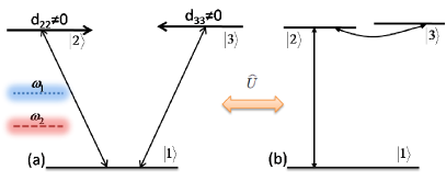
Figure 1: Three-level atomic structures for (a) $V$ type with mean dipole moments in the excited states and (b) $\Gamma$ configuration with the coupling transition between the excited states. The considered configurations are unitary equivalent to each other.

The Hamiltonian for the system within semiclassical dipole approximation is given in form

$$\widehat{H}=\varepsilon_{1}|1\rangle\langle 1|+\left(\varepsilon_{2}+V_{22}\right)|2\rangle\langle 2|+\left(\varepsilon_{3}+V_{33}\right)|3\rangle\langle 3|$$

$$+\left(V_{12}|1\rangle\langle 2|+V_{13}|1\rangle\langle 3|+\mathrm{h.c.}\right),$$ (1)

where, $\varepsilon_{1}$, $\varepsilon_{2}$ and $\varepsilon_{3}$ are the energies of the stationary states $\left|1\right\rangle$, $\left|2\right\rangle$ and $\left|3\right\rangle$ respectively, and

$$V_{\eta\nu}=-d_{\eta\nu}\left(E_{1}\cos\left(\omega_{1}t+\varphi\right)+E_{2}\cos\left(\omega_{2}t\right)\right),$$ (2)

is the interaction part of the Hamiltonian with a real matrix element of the electric dipole moment projection $d_{\eta\nu}$ $=\mathbf{d}_{\eta\nu}\mathbf{\cdot\hat{e}}$, and $E_{1,2}$ are slowly varying amplitudes of linearly polarized laser fields, with unit polarization vector $\mathbf{\hat{e}}$ and constant relative phase $\varphi$. The diagonal terms in (2) describe the interaction due to the mean dipole moments and are crucial for effective multiphoton coupling.

We consider Schrödinger equation

$$i\frac{\partial\left|\Psi(t)\right\rangle}{\partial t}=\hat{H}\left|\Psi(t)\right\rangle,$$ (3)

with Hamiltonian (1) at the resonance $\left|\delta_{2,3}\right|\ll\omega_{1,2}$ for efficient multiphoton coupling. The resonance detunings are given by relations

$$\delta_{2,3}=\varepsilon_{1}-\varepsilon_{2,3}+n_{1}\omega_{1}+n_{2}\omega_{2},$$ (4)

for $\left(n_{1},n_{2}\right)$ pair of photon numbers. Here and below, unless otherwise stated, atomic units ($\hbar=e=m_{e}=1$) are employed.

Our method of solving the Schrödinger equation with Hamiltonian (1) has been described in detail in AAM4 , and will be excluded here. The time-dependent wave function can be expressed as

$$|\Psi\left(t\right)\rangle=\left(\overline{a}_{1}(t)+\alpha_{1}(t)\right)e^{-i\varepsilon_{1}t}|1\rangle$$

$$+\left(\overline{a}_{2}(t)+\alpha_{2}(t)\right)e^{-i\left(\varepsilon_{2}t+\int_{0}^{t}V_{22}dt\right)}|2\rangle$$

$$+\left(\overline{a}_{3}(t)+\alpha_{3}(t)\right)e^{-i\left(\varepsilon_{3}t+\int_{0}^{t}V_{33}dt\right)}|3\rangle,$$ (5)

where $\overline{a}_{i}(t)$ are the time-averaged probability amplitudes and $\alpha_{i}(t)$ are rapidly changing functions on the scale of waves’ periods. Depending on the ratio of frequencies $\omega_{1}/\omega_{2}$ the resonant condition (4) can hold for a single pair of photon numbers -normal resonance or can also be satisfied by diverse pairs of photons numbers (in principle infinity) -degenerate resonance. Let us first consider the case of normal resonance. Hence, if resonant condition holds for a pair ($n,m$) then assuming the smooth turn-on of the pump waves, the relation between rapidly oscillating and slow oscillating parts of the probability amplitudes can be written

$$\alpha_{1}(t)=\bar{a}_{2}\sum_{\begin{subarray}{c}s_{1},s_{2}=-\infty,\\ \left(s_{1},s_{2}\right)\neq\left(0,0\right)\end{subarray}}^{\infty}\zeta_{12}(s_{1},s_{2})e^{i\left(s_{1}\omega_{1}+s_{2}\omega_{2}\right)t}$$

$$+\bar{a}_{3}\sum_{\begin{subarray}{c}s_{1},s_{2}=-\infty,\\ \left(s_{1},s_{2}\right)\neq\left(0,0\right)\end{subarray}}^{\infty}\zeta_{13}(s_{1},s_{2})e^{i\left(s_{1}\omega_{1}+s_{2}\omega_{2}\right)t},$$ (6)

$$\alpha_{2}(t)=-\bar{a}_{1}\sum_{\begin{subarray}{c}s_{1},s_{2}=-\infty,\\ \left(s_{1},s_{2}\right)\neq\left(0,0\right)\end{subarray}}^{\infty}\zeta_{12}^{\ast}(s_{1},s_{2})e^{-i\left(s_{1}\omega_{1}+s_{2}\omega_{2}\right)t},$$ (7)

$$\alpha_{3}(t)=-\bar{a}_{1}\sum_{\begin{subarray}{c}s_{1},s_{2}=-\infty,\\ \left(s_{1},s_{2}\right)\neq\left(0,0\right)\end{subarray}}^{\infty}\zeta_{13}^{\ast}(s_{1},s_{2})e^{-i\left(s_{1}\omega_{1}+s_{2}\omega_{2}\right)t},$$ (8)

where

$$\zeta_{12}(s_{1},s_{2})=\frac{d_{12}}{d_{22}}\frac{\left(s_{1}+n\right)\omega_{1}+\left(s_{2}+m\right)\omega_{2}}{s_{1}\omega_{1}+s_{2}\omega_{2}}$$

$$\times J_{s_{1}+n}\left(\frac{d_{22}E_{1}}{\omega_{1}}\right)J_{s_{2}+m}\left(\frac{d_{22}E_{2}}{\omega_{2}}\right)e^{i\left(s_{1}+n\right)\varphi},$$ (9)

and

$$\zeta_{13}(s_{1},s_{2})=\frac{d_{13}}{d_{33}}\frac{\left(s_{1}+n\right)\omega_{1}+\left(s_{2}+m\right)\omega_{2}}{s_{1}\omega_{1}+s_{2}\omega_{2}}$$

$$\times J_{s_{1}+n}\left(\frac{d_{33}E_{1}}{\omega_{1}}\right)J_{s_{2}+m}\left(\frac{d_{33}E_{2}}{\omega_{2}}\right)e^{i\left(s_{1}+n\right)\varphi}.$$ (10)

In deriving these equations we have applied well-known Jacobi–Anger expansion via Bessel functions:

$$e^{iZ\sin\alpha}=\sum\limits_{s=-\infty}^{\infty}J_{s}\left(Z\right)e^{is\alpha}.$$ (11)

Now let us proceed to the case of degenerate resonance. Particularly if $\omega_{1}/\omega_{2}=k$, where $k$ is an integer number, then there are many channels of resonance transitions and one should take into account all possible transitions and the relation between rapidly oscillating and slow oscillating parts of the probability amplitudes can be written

$$\alpha_{1}(t)=\sum_{\begin{subarray}{c}s_{1},s_{2}=-\infty,\\ s_{2}\neq 0\end{subarray}}^{\infty}\left[\bar{a}_{2}\frac{d_{12}}{d_{22}}J_{s_{1}}\left(\frac{d_{22}E_{1}}{k\omega_{2}}\right)J_{s_{2}+n-ks_{1}}\left(\frac{d_{22}E_{2}}{\omega_{2}}\right)\right.$$

$$\left.+\bar{a}_{3}\frac{d_{13}}{d_{33}}J_{s_{1}}\left(\frac{d_{33}E_{1}}{k\omega_{2}}\right)J_{s_{2}+n-ks_{1}}\left(\frac{d_{33}E_{2}}{\omega_{2}}\right)\right]\frac{s_{2}+n}{s_{2}}e^{is_{1}\varphi}e^{is_{2}\omega_{2}t},$$ (12)

$$\alpha_{2}(t)=-\bar{a}_{1}\frac{d_{12}}{d_{22}}\sum_{\begin{subarray}{c}s_{1},s_{2}=-\infty,\\ s_{2}\neq 0\end{subarray}}^{\infty}J_{s_{1}}\left(\frac{d_{22}E_{1}}{k\omega_{2}}\right)J_{s_{2}+n-ks_{1}}\left(\frac{d_{22}E_{2}}{\omega_{2}}\right)\frac{s_{2}+n}{s_{2}}e^{-is_{1}\varphi}e^{-is_{2}\omega_{2}t},$$ (13)

$$\alpha_{3}(t)=-\bar{a}_{1}\frac{d_{13}}{d_{33}}\sum_{\begin{subarray}{c}s_{1},s_{2}=-\infty,\\ s_{2}\neq 0\end{subarray}}^{\infty}J_{s_{1}}\left(\frac{d_{33}E_{1}}{k\omega_{2}}\right)J_{s_{2}+n-ks_{1}}\left(\frac{d_{33}E_{2}}{\omega_{2}}\right)\frac{s_{2}+n}{s_{2}}e^{-is_{1}\varphi}e^{-is_{2}\omega_{2}t},$$ (14)

where $n$ is given by resonance condition

$$\varepsilon_{1}-\varepsilon_{2,3}+n\omega_{2}\simeq 0.$$ (15)

In the Schrödinger picture the coherent part of the dipole spectrum is expressed as follows EF :

$$S_{c}(\omega)=\left|\int_{-\infty}^{\infty}dte^{-i\omega t}\left\langle d(t)\right\rangle\right|^{2},$$ (16)

where

$$\left\langle d(t)\right\rangle=\left\langle\Psi(t)\right|\mathbf{\hat{e}\cdot\hat{d}(0)}\left|\Psi(t)\right\rangle,$$ (17)

is the time-dependent expectation value of dipole operator. With the help of wave function (5) the expectation value of the dipole operator (17) can be written as

$$\left\langle d(t)\right\rangle=\frac{d_{22}}{2}\left|\overline{a}_{2}(t)+\alpha_{2}(t)\right|^{2}+\frac{d_{33}}{2}\left|\overline{a}_{3}(t)+\alpha_{3}(t)\right|^{2}$$

$$+d_{12}\left(\overline{a}_{1}^{\ast}(t)+\alpha_{1}^{\ast}(t)\right)\left(\overline{a}_{2}(t)+\alpha_{2}(t)\right)\sum\limits_{s_{1},s_{2}=-\infty}^{\infty}J_{s_{1}}\left(\frac{d_{22}E_{1}}{\omega_{1}}\right)J_{s_{2}}\left(\frac{d_{22}E_{2}}{\omega_{2}}\right)e^{i\left(s_{1}\omega_{1}+s_{2}\omega_{2}\right)t}e^{i\left(\varepsilon_{1}-\varepsilon_{2}\right)t+is_{1}\varphi}$$

$$+d_{13}\left(\overline{a}_{1}^{\ast}(t)+\alpha_{1}^{\ast}(t)\right)\left(\overline{a}_{3}(t)+\alpha_{3}(t)\right)\sum\limits_{s_{1},s_{2}=-\infty}^{\infty}J_{s_{1}}\left(\frac{d_{33}E_{1}}{\omega_{1}}\right)J_{s_{2}}\left(\frac{d_{33}E_{2}}{\omega_{2}}\right)e^{i\left(s_{1}\omega_{1}+s_{2}\omega_{2}\right)t}e^{i\left(\varepsilon_{1}-\varepsilon_{3}\right)t+is_{1}\varphi}+\mathrm{c.c.}.$$ (18)

Combining the solution for slow oscillating parts of the probability amplitudes with (9), (10) and (18) one can calculate analytically the expectation value of the dipole operator for an arbitrary initial atomic state. The Fourier transform of $\left\langle d(t)\right\rangle$ gives the coherent part of the dipole spectrum.

The solution for slow oscillating parts of the probability amplitudes analytically is very complicated and in order to reveal the physics of multiphoton resonant excitation process let us consider systems with inversion symmetry: $d_{12}=-d_{13}\equiv d_{tr}$ and $d_{22}=-d_{33}\equiv d$. As is seen from (18), for effective harmonic generation in certain resonance conditions one should provide considerable population transfer between the atomic states $\left|1\right\rangle$ and upper levels $\left|2\right\rangle$ and $\left|3\right\rangle$. Dynamic Stark shifts can take the states off resonance, so appropriate detunings for compensation are chosen.

Let us first consider the case of normal resonance. For the system initially situated in the ground state, the solution for slow oscillating parts of the probability amplitudes is AAM4 :

$$\overline{a}_{1}(t)=e^{-i2\Delta t}\sin(\Omega_{R}t),$$ (19)

$$\overline{a}_{2}(t)=\frac{(-1)^{n+m}}{i\sqrt{2}}e^{-i2\Delta t}\sin(\Omega_{R}t),$$ (20)

$$\overline{a}_{3}(t)=\frac{1}{i\sqrt{2}}e^{-i2\Delta t}\sin(\Omega_{R}t),$$ (21)

where $\Delta$ describes dynamic Stark shifts

$$\Delta\equiv\left(\frac{d_{tr}}{d}\right)^{2}\sum_{\begin{subarray}{c}s_{1},s_{2}=-\infty,\\ \left(s_{1},s_{2}\right)\neq\left(n,m\right)\end{subarray}}^{\infty}\frac{\left(s_{1}\omega_{1}+s_{2}\omega_{2}\right)^{2}}{(s_{1}-n)\omega_{1}+(s_{2}-m)\omega_{2}}$$

$$\times J_{s_{1}}^{2}\left(\frac{dE_{1}}{\omega_{1}}\right)J_{s_{2}}^{2}\left(\frac{dE_{2}}{\omega_{2}}\right).$$ (22)

and $\Omega_{R}$ expresses the frequency of Rabi oscillations

$$\Omega_{R}\equiv\left|2\sqrt{2}\frac{d_{tr}}{d}J_{n}\left(\frac{dE_{1}}{\omega_{1}}\right)J_{m}\left(\frac{dE_{2}}{\omega_{2}}\right)\right|.$$ (23)

Replacing the probability amplitudes in (18) by the corresponding expressions (19)-(21) and taking into account the relations (6)-(8) one can derive the final analytical expression for $\left\langle d(t)\right\rangle$. As is seen from Eq. (22), the dynamic Stark shift is proportional to the ratio $d_{tr}^{2}/d^{2}$, while the multiphoton coupling is proportional to $d_{tr}/d$. Since large dynamic Stark shifts are detrimental for maintenance of considerable population transfer, here we consider systems with $\left|d_{tr}/d\right|\ll 1$. Taking into account the smallness of the parameter $\left|d_{tr}/d\right|$, from (18) at the first approximation we derive the following compact analytic formula:

$$\left\langle d(t)\right\rangle=\sum_{\begin{subarray}{c}s_{1},s_{2}=-\infty,\\ \left(s_{1},s_{2}\right)\neq\left(0,0\right)\end{subarray}}^{\infty}D_{s_{1}s_{2}}\sin((s_{1}\omega_{1}+s_{2}\omega_{2})t+s_{1}\varphi),$$ (24)

where

$$D_{s_{1}s_{2}}=\frac{d_{tr}}{\sqrt{2}}\sin(\Omega_{R}t)\frac{n\omega_{1}+m\omega_{2}}{s_{1}\omega_{1}+s_{2}\omega_{2}}(1-(-1)^{s_{1}+s_{2}})$$

$$\times J_{s_{1}+n}\left(\frac{dE_{1}}{\omega_{1}}\right)J_{s_{2}+m}\left(\frac{dE_{2}}{\omega_{2}}\right).$$ (25)

As we can see from (24), (25), the spectrum consists of doublets $s_{1}\omega_{1}+s_{2}\omega_{2}\pm\Omega_{R}$. At that only harmonics with odd sum of harmonic numbers $s_{1}+s_{2}$ are existed, as it was expected because of inversion symmetry of the considered problem.

Now let us consider the degenerate resonance. Particularly if $\omega_{1}/\omega_{2}=k$, where $k$ is odd, the dipole expectation value can be obtained from Eqs. (12)-(14), (18) and is given as:

$$\left\langle d(t)\right\rangle=\frac{d_{tr}n}{\sqrt{2}}\sum_{\begin{subarray}{c}s_{1},s_{2}=-\infty,\\ s_{2}\neq 0\end{subarray}}^{\infty}J_{s_{2}+n-ks_{1}}\left(\frac{dE_{2}}{\omega_{2}}\right)J_{s_{1}}\left(\frac{dE_{1}}{k\omega_{2}}\right)$$

$$\times\frac{1-(-1)^{s_{2}}}{s_{2}}\sin(\Omega_{R}^{\prime}t)\sin(s_{2}\omega_{2}t+s_{1}\varphi),$$ (26)

where Rabi frequenc is given as:

$$\Omega_{R}^{\prime}\equiv\left|2\sqrt{2}\frac{d_{tr}}{d}n\omega_{2}\sum\limits_{s}J_{n-ks}\left(\frac{dE_{2}}{\omega_{2}}\right)J_{s}\left(\frac{dE_{1}}{k\omega_{2}}\right)\right|.$$ (27)

The spectrum is noticeably different for even $k$. In particular, for bichromatic field with frequencies $\omega$ and $2\omega$ dipole spectrum contains also even harmonics of the main frequency, tunable low-frequency (much smaller than $\omega$) part and six hyper-Raman lines per harmonic. Dipole moment expectation value is expressed by very bulky formula and will not be given here.

III NUMERICAL RESULTS AND DISCUSSION

In this section we present numerical calculations for hydrogen atom and homonuclear diatomic molecular ion $N_{2}^{4+}$ Gib2 with the specific parameters of available laboratory lasers. The numerical results will be compared with exact results of the dipole spectrum to estimate accuracy and applicability of generalized rotating wave approximation. The time-dependent Schrödinger equation for three-level model with Hamiltonian (1) are considered. The solution for the probability amplitudes has been obtained using Runge-Kutta algorithm and scattering spectrum is estimated by applying the fast Fourier transform method NR . For smooth turn-on of the laser fields, we consider envelopes with hyperbolic tangent $\tanh(t/\tau)$ temporal shape, where $\tau$ characterizes the turn-on time and chosen to be $40\pi/\omega_{2}$. It is assumed that quantum systems are initially in the ground state $\left|1\right\rangle$. For both systems the main transitions fall in the vacuum ultraviolet range. Thus, $\varepsilon_{1}-\varepsilon_{2,3}\simeq 0.375$ $\mathrm{a.u}$. and $\simeq 0.6838$ $\mathrm{a.u}$. for hydrogen atom and ion $N_{2}^{4+}$, respectively. This is a spectral domain where strong coherent radiation is difficult to generate and two or higher photon multicolor resonant excitation is of interest.

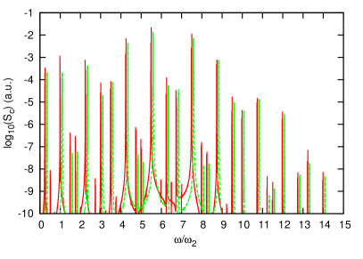
Figure 2: (Color online) The logarithm of the coherent part of the spectrum $S_{C}(\omega)$ at four-photon two-color resonance ($n=2,m=2$) of hydrogen atom with $E_{1}=E_{2}=0.02$ $\mathrm{a.u}$, $\omega_{1}=0.13$ $\mathrm{a.u}$, and $\omega_{2}=0.0579$ $\mathrm{a.u.}$ The solid (red) line corresponds to numerical calculations; the dashed (green) line corresponds to the approximate solution (for better visibility the latter has been slightly shifted to the right).

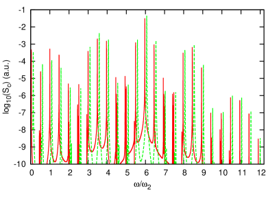
Figure 3: (Color online) The logarithm of the coherent part of the spectrum $S_{C}(\omega)$ at five-photon two-color resonance ($n=2,m=3$) of hydrogen atom with $E_{1}=E_{2}=0.02$ $\mathrm{a.u}$, $\omega_{1}=0.0935$ $\mathrm{a.u}$, and $\omega_{2}=0.063$ $\mathrm{a.u.}$ The solid (red) line corresponds to numerical calculations; the dashed (green) line corresponds to the approximate solution.

Figure 2 displays the multicolor harmonic and wave-mixing emission rate (coherent part) as a function of the ratio $\omega/\omega_{2}$ (we assume $\omega_{2}<\omega_{1}$ and $\varphi=0$) at the four-photon two-color resonant excitation of hydrogen atom with XeF excimer (351 nm, $n=2$) and Ti:sapphire (780 nm, $m=2$) laser systems with $E_{1}=E_{2}=0.02$ $\mathrm{a.u}$.. For the hydrogen atom $d_{tr}=0.5267$ $\mathrm{a.u}$. and $d=3.0$ $\mathrm{a.u}$. Here and below, for the chosen parameters the dynamic Stark shift is compensated. The latter provides almost complete population transfer. The solid (red) line corresponds to numerical calculations, while the dashed (green) line corresponds to the approximate expression (24). Note that the numerical and analytical calculations coincide with high accuracy, so for visual convenience to distinguish these curves the spectrum corresponding to analytical calculations (24) has been slightly shifted to the right for Figs. 2-5.

Figure 3 displays the multicolor harmonic and wave-mixing emission rate at the five-photon two-color resonant excitation of hydrogen atom with Ar+ (488 nm, $n=2$) and Ti:sapphire (724 nm, $m=3$) laser systems with $E_{1}=E_{2}=0.02$ $\mathrm{a.u}$.

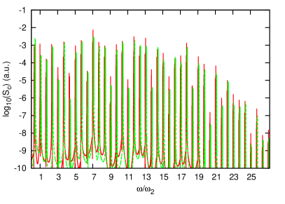
Figure 4: (Color online) The logarithm of the coherent part of the spectrum $S_{C}(\omega)$ at seven-photon two-color resonance ($n=4,m=3$) of N${}_{2}^{4+}$ molecular ion with $E_{1}=E_{2}=0.07$ $\mathrm{a.u}$, $\omega_{1}=0.13$ $\mathrm{a.u}$, and $\omega_{2}=0.05562$ $\mathrm{a.u.}$ The solid (red) line corresponds to numerical calculations; the dashed (green) line corresponds to the approximate solution.

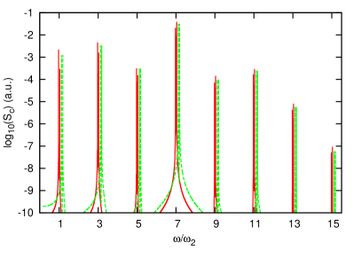
Figure 5: (Color online) The radiation spectrum at two-color resonant excitation of hydrogen atom with laser fields $E_{1}=E_{2}=0.02$ $\mathrm{a.u}$, $\omega_{1}=3\omega_{2}$, and $\omega_{2}=0.05371$ $\mathrm{a.u..}$

In Fig. 4 we plot harmonic/wave-mixing emission rate at the seven-photon two-color resonant excitation of N${}_{2}^{4+}$ molecular ion with XeF excimer (351 nm, $n=4$) and Ti:sapphire (820 nm, $m=3$) laser systems with $E_{1}=E_{2}=0.07$ $\mathrm{a.u}$. For this system we take $d_{tr}=0.3536$ $\mathrm{a.u}$. and $d=3.0$ $\mathrm{a.u}$..

For a degenerate case of resonance in Fig. 5 we plot harmonic/wave-mixing emission rate at $\omega_{1}=3\omega_{2}$ with $\omega_{2}=0.05371$ $\mathrm{a.u}$. (849nm) at waves’ electric fields $E_{1}=E_{2}=0.02$ $\mathrm{a.u}$.. For the case $\omega_{1}=2\omega_{2}$ the radiation spectrum is similar to non-degenerate case. However, there are a few differences. Scattering spectrum is richer in satellites of multicolor harmonics, in addition there is low-frequency radiation on Rabi frequencies. In Fig. 6 we plot low-frequency part of radiation spectrum. Here, the presented triplet which can be tuned by laser parameters lies in THz/IR region.

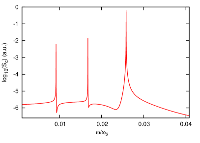
Figure 6: (Color online) Low-frequency part of radiation spectrum at two-color resonant excitation of hydrogen atom with laser fields $E_{1}=E_{2}=0.025$ $\mathrm{a.u}$, $\omega_{1}=2\omega_{2}$, and $\omega_{2}=0.06267$ $\mathrm{a.u..}$

As is seen from these figures in the coherent spectrum there are as harmonics of the individual waves as well as frequencies with sum/difference components and its harmonics, in accordance with the analytical ansatz (26). From Eq. (25) it is clear that for effective harmonic generation one should provide large dipole interaction energy $dE_{1,2}\gtrsim\omega_{1,2}$, since the Bessel function exponentially decreases with increasing index at the given argument. The Bessel function $J_{s}\left(Z\right)$ at large argument values reaches its maximum at $s\sim Z$. Thus, the cutoff frequency depends linearly on the amplitudes of the laser fields.

Let us make some estimations for reasonable interaction parameters. The average number of photons at the frequency $\omega$ emitted at each lasers shots of duration $\tau$, Rayleigh length $L_{R}$ on the atomic/molecular ensemble of density $N_{a}$ can be estimated as AAM2 :

$$N_{\omega}\simeq\frac{\left(2\pi\right)^{2}}{\hbar}S_{c}(\omega)N_{a}^{2}L_{R}^{3}\tau$$

The incident pulse duration is assumed to be $50$ $\mathrm{ps}$, the Rayleigh length is taken to be $L_{R}=1\ \mathrm{mm}$, and for emitters density we assume $N_{a}\simeq 5\times 10^{17}$cm^-3. For the setup of Figs. 3 and 4 with the chosen parameters, the average number of radiated photons at frequencies up to $\omega\simeq 20\omega_{2}$ per shot is $N_{\omega}\sim 10^{12}$, which is two orders of magnitude larger than what one expects to achieve with tunneling harmonics generation Huillier .

IV SUMMARY

We have presented a theoretical treatment of the multicolor harmonics generation and wave-mixing in a three-level atomic-molecular system under two-color multiphoton resonant excitation. The coherent part of the dipole spectrum was investigated. With the help of an approximate analytical expression for the dynamic wave function of a three-level atom driven by intense laser fields, we obtained an analytical expression for the time-dependent expectation value of the dipole operator. Then the results obtained were applied to the hydrogen atom and homonuclear diatomic molecular ion. The spectrum shows harmonics of the individual waves as well as frequencies with sum/difference components and its harmonics. These peaks have quite large amplitudes. The latter is the result of multiphoton resonant interaction of the system with the driving bichromatic laser radiation due to the mean dipole moment in the stationary states. The cutoff frequency depends linearly on the amplitudes of laser fields. The presence of the second laser field can make easier the implementation of efficient population transfer and harmonic generation as well as allows generation of new frequencies. Analytical calculations in the generalized rotating wave approximation AM ; AAM4 allow an explanation of the obtained spectrum. The numerical simulations are in good agreement with the analytical results. The considered scheme may serve as a promising method for efficient production of multicolor high harmonics. It should be noted that the obtained results can be applied to other systems in diverse domains of the electromagnetic spectrum.

- (1) N. Bloembergen, Nonlinear Optics (Benjamin, New York, 1965); R. W. Boyd, Nonlinear Optics (Academic Press, San Diego, 2008).
- (2) A. McPherson, G. Gibson, H. Jara, U. Johann, T. S. Luk, I. A. McIntyre, K. Boyer, and C. K. Rhodes, J. Opt. Soc. Am. B 4, 595 (1987); . M. Ferray, A. L’Huillier, X. F. Li, L. A. Lompre, G. Mainfray and C. Manus, J. Phys. B 21, L31 (1988).
- (3) E. Seres, J. Seres, and C. Spielmann, Applied Physics Letters 89, 181919 (2006).
- (4) M.-C. Chen, P. Arpin, T. Popmintchev, M. Gerrity, B. Zhang, M. Seaberg, D. Popmintchev, M. M. Murnane, and H. C. Kapteyn, Phys. Rev. Lett. 105, 173901 (2010).
- (5) T. Popmintchev et.al., Science 336, 1287 (2012).
- (6) M. Protopapas, C. H. Keitel, and P. L. Knight, Rep. Prog. Phys. 60, 389 (1997); P. Saliéres A. L’Huillier, P. Antoine, and M. Lewenstein, Adv. At., Mol., Opt. Phys. 41, 83 (1999); T. Brabec and F. Krausz, Rev. Mod. Phys. 72, 545 (2000); P. Agostini and L. F. DiMauro, Rep. Prog. Phys. 67, 813 (2004); M. C. Kohler, T. Pfeifer, K. Z. Hatsagortsyan, and C. H. Keitel, Adv. At. Mol. Opt. Phys. 61, 159 (2012).
- (7) Z. H. Kafafi, J. R. Lindle, R. G. S. Pong, F. J. Bartoli, L. J. Lingg, and J. Milliken, Chem. Phys. Lett. 188, 492 (1992); P. Haljan, T. Fortier, P. Hawrylak, P. B. Corkum, and M. Yu. Ivanov, Laser Phys. 13, 452 (2003); G. P. Zhang, Phys. Rev. Lett. 95, 047401 (2005); D. Golde, T. Meier, and S. W. Koch, Phys. Rev. B 77, 075330 (2008).
- (8) H. K. Avetissian, B. R. Avchyan, and G. F. Mkrtchian, Phys. Rev. A 77, 023409 (2008).
- (9) H. K. Avetissian, B. R. Avchyan, and G. F. Mkrtchian, J. Phys. B 45, 025402 (2012).
- (10) H. K. Avetissian, B. R. Avchyan, and G. F. Mkrtchian, Phys. Rev. A 90, 053812 (2014).
- (11) G. N. Gibson, Phys. Rev. A 91, 033411 (2015).
- (12) A. L’Huillier, K. J. Schafer, and K. C. Kulander, J. Phys. B 24, 3315 (1991); Ph. Balcou, C. Cornaggia, A. S. L. Gomes, L. A. Lompre, and A. L’Huillier, ibid. 25, 4467 (1992).
- (13) P. B. Corkum, Phys. Rev. Lett. 71, 1994 (1993); K. J. Schafer, B. Yang, L. F. DiMauro, and K. C. Kulander, Phys. Rev. Lett. 70, 1599 (1993); M. Lewenstein, Ph. Balcou, M. Yu. Ivanov, Anne L’Huillier, and P. B. Corkum, Phys. Rev. A 49, 2117 (1994); V. Averbukh, O. E. Alon, and N. Moiseyev, Phys. Rev. A 64, 033411 (2001); C. Figueira de Morisson Faria and I. Rotter, Phys. Rev. A 66, 013402 (2002).
- (14) H. K. Avetissian and G. F. Mkrtchian, Phys. Rev. A 66, 033403 (2002).
- (15) H. K. Avetissian, G. F. Mkrtchian, and M. G. Poghosyan, Phys. Rev. A 73, 063413 (2006).
- (16) H. K. Avetissian, B. R. Avchyan, and G. F. Mkrtchian, Phys. Rev. A 74, 063413 (2006).
- (17) M. A. Kmetic and W. J. Meath, Phys. Lett. A 108, 340 (1984); A. Brown, W. J. Meath, and P. Tran, Phys. Lett. A 63, 013403 (2000); A. Brown, W. J. Meath and P. Tran, Phys. Rev. A 65, 063401 (2002).
- (18) G. N. Gibson, M. Li, C. Guo, and J. P. Nibarger, Phys. Rev. A 58, 4723 (1998); G. N. Gibson, Phys. Rev. Lett. 89, 263001 (2002).
- (19) H. K. Avetissian, A. K. Avetissian, G. F. Mkrtchian, O. V. Kibis, J. Nanophoton. 9, 093064 (2015); JETP 121, 925 (2015).
- (20) W. D. Oliver, Y. Yu, J. C. Lee, K. K. Berggren, L. S. Levitov, and T. P. Orlando, Science 310, 1653 (2005).
- (21) A. Wallraff et.al., Nature 431, 162 (2004).
- (22) L.D. Landau and E.M. Lifshitz, Quantum Mechanics (Pergamon Press, Oxford, 1977).
- (23) J. H. Eberly and M. V. Fedorov, Phys. Rev. A 45, 4706 (1992).
- (24) L. Allen and J. H. Eberly, Optical Resonance and Two-Level Atoms (Wiley-Interscience, New York, 1975).
- (25) W. H. Press, S. A. Teukolsky, W. T. Vetterling, and B. P. Flannery, Numerical Recipes: The Art of Scientific Computing ( Cambridge University Press, Cambridge, 2007).