Tessellations derived from random geometric graphs

Abstract

In this paper we consider a random partition of the plane into cells, the partition being based on the nodes and links of a random planar geometric graph. The resulting structure generalises the random tessellation hitherto studied in the literature. The cells of our partition process, possibly with holes and not necessarily closed, have a fairly general topology summarised by a functional which is similar to the Euler characteristic. The functional can also be extended to certain cell-unions which can arise in applications. Vertices of all valencies, $0,1,2,...$ are allowed. Many of the formulae from the traditional theory of random tessellations with convex cells, are made more general to suit this new structure. Some motivating examples of the structure are given.

1. Introduction

In this paper we consider a very general type of stationary random ‘tessellation’ in the plane, one which might be called a random planar partitioning (RPP). Later in this introduction, we shall describe this general structure but, as a foundation, we firstly review the status of the random tessellation literature.

Basic information about convex-celled tessellations: The theory of planar random tessellations has evolved over the years partly through particular models and partly via model-free studies which assume only stationarity and local finiteness. Often researchers of model-free tessellations have added a convexity assumption — cells must be convex — and also a statement about the closed or open status of the cells; see [1], [2], [4], [6], [13], [14] and [19].

We commence our discussion with the version where all cells in the model-free tessellation are closed, bounded and convex. Firstly we define a tessellation in this context.

Definition 1

: A tessellation  of the plane is a locally-finite collection of compact convex cells, each of positive area, which cover the plane and overlap only on cell boundaries. The union of the cell boundaries is called the tessellation frame. Each cell, being a polygon, has sides and corners; they lie on the frame. The union (taken over all cells) of cell corners is a collection of points in the plane called the vertices of the tessellation. Those closed line-segments which are contained in the frame, have a vertex at each end and no vertices in their relative-interior are called edges of the tessellation. The number of edges emanating from a vertex is called the valency of that vertex.

Whereas no vertices can lie in the interior of an edge, some vertices might lie in the interior of a cell-side.

Definition 2

: Vertices which lie in the relative interior of a cell-side are called $\pi$-vertices. The name arises because in such vertices one of the angles between consecutive emanating edges is $\pi$.

The focus of attention in many studies of planar tessellations and tilings has been the side-to-side case.

Definition 3

: A tessellation is side-to-side if each side of any polygonal cell in the tessellation coincides with a side of another cell. Alternatively, we say that a tessellation is side-to-side if it has no $\pi$-vertices.

Introducing randomness, stationarity and ergodicity: Let $\Omega$ be the space of tessellations (each $\omega\in\Omega$ conforming to Definition 1). A convex-celled random tessellation is a randomly selected (or randomly constructed) entity $\omega\in\Omega$. More precisely, we place a probability measure $\mathbb{P}$ on a suitably-large class $\mathcal{Q}$ of subsets of $\Omega$. So the triple $(\Omega,\mathcal{Q},\mathbb{P})$ is our random convex-celled tessellation. The expectation associated with $\mathbb{P}$ is written as $\mathbb{E}(\cdot)$.

For $x,\ t\in\mathrm{R}^{2}$ define the translation operator $T^{t}:x\rightarrow x+t$. Thus $T^{t}$, which is also defined on $\Omega$, translates any realisation $\omega$ by $t$. We assume that the random tessellation process is stationary and ergodic, via the assumption that $T^{t}$ (when defined on $\mathcal{Q}$) is a measure-preserving and ergodic operator. Intuitively, ‘measure-preserving’ means that the statistical properties of the structure are invariant under translation. Ergodicity has implications when taking large-domain spatial averages in the random process; it implies that spatial averages (for example, the average vertex valency) and various proportions (for example, the proportion of vertices which are $\pi$-vertices) calculated inside the ball $B_{r}$, of radius $r$ and with centre at the planar origin, converge with probability one to a constant as $r\rightarrow\infty$.

There are three basic types of ergodic tessellation. In one type, the periodic tessellations, there is a sub-collection of cells which forms a repeating structure; the full tessellation covering the whole plane is made up of suitably translated copies of this structure. It is clear that spatial averaging applies; for example, the large-domain limit of average cell area will obviously converge to the average cell area within the ‘repeating sub-collection’. To make such a periodic tessellation stationary, one places it on the plane so that the planar origin is uniformly distributed within one copy of the repeating sub-collection.

In the second ergodic type, the mixing tessellations, the method of constructing the stationary random tessellation is such that features which are a considerable distance apart are effectively statistically independent. The geometry of a tessellation will, of course, impose a short-range dependence but this decreases with distance in this type of ergodic tessellation, in the limit (as distance tends to infinity) to complete independence. As is well known, averaging over independent entities leads to almost-sure convergence to a constant. For mixing tessellations the short-range dependencies are dominated by the vastly greater number of long-range ‘independencies’ — and convergence to a constant still occurs.

As for the third type, these are combinations of the first two — for example, a periodic tessellation modified by random operations which have a tendency toward independence as distance increases. There are many ways to combine the notions of periodicity and mixing whilst retaining the large-domain limiting condition that comes with ergodicity.

Relaxing the convexity assumption: One can generalise slightly the tessellation that we have defined in Definition 1, relaxing convexity of the cells and permitting vertices of valency $2$, but retaining line-segment edges. So cells remain as simple polygons, though not necessarily convex. Such model-free tessellations have been studied in [15], [18] and [8].

The tiling literature also allows non-convex cells (see Grünbaum and Shephard [11]). The cells, assumed closed, may have fairly general shapes that are isomorphic to a closed planar disk. Whilst this allows considerable freedom in the type of non-convex cell, the other regularity conditions used by the tilers (N.2 and N.3 imposed on page 121 in [11]) are far too restrictive for us, especially with our emphasis on random tessellations. Grünbaum and Shephard were mainly concerned with non-random tilings; N.2 and N.3 are highly appropriate regularity conditions for non-random tilings.

Another style of generalisation is due to Zähle and co-authors Weiss and Leistritz ([20], [21] and [12]). In the most recent of these studies, the edges and cells are simply-connected compact submanifolds (of dimensions $1$ and $2$ respectively imbedded in $\mathrm{R}^{2}$) with boundary. Various rules govern how cells, edges and vertices interconnect. These rules, listed below, come from the theory of $d$-dimensional cell-complexes with $d=2$.

1. The intersection of two cells is contained in the boundary of each of these cells; it is either empty or it is an edge or it is an isolated vertex.

2. The intersection of two edges is either empty or it is a vertex which lies at a terminus of each of these edges.

3. Any edge is contained in the boundary of some cell.

4. Any vertex is located at a terminus of some edge.

5. The boundary of any cell is the finite union of some edges.

6. The boundary of an edge is the union of two vertices.

So the edges can be curved in the Zähle/Weiss/Leistritz theory, possibly with discontinuities of slope, provided no vertex is positioned at these ‘corners’ of the curve. Thus vertices of valency $2$ are not allowed and, as we shall see, much of the complexity that we introduce in the next section is not allowed in their theory.

2. Generalising the planar graph

In order to understand other natural models for partitioning the plane, we have recognised the need to generalise further than can be achieved by the techniques described above. We do this by casting the discussion in terms of planar graphs.

The frame of a tessellation complying with Definition 1 can be viewed as an infinite planar graph. This graph has some imposed geometry and some topological constraints. As is well known, a planar graph has nodes placed in the plane, with links connecting some pairs of distinct nodes. In a graph which is the frame of a ‘Definition 1 tessellation’, the tessellation vertices (which must have valency $\geq 3$) play the role of the graph’s nodes whilst the tessellation edges are the links, assumed non-directed. The links must be line-segments whose relative interiors are disjoint. The polygonal cells of the tessellation play the role of the graph’s faces; so these faces are convex, closed and bounded. Terminology such as ‘node valency’ and ‘$\pi$-node’ become defined on the graph via their tessellation meaning.

We now allow the infinite planar graph to be much more general, whilst retaining the rule that each link is a line-segment which does not intersect other links except at its terminating nodes. Firstly a countable collection of distinct points in $\mathrm{R}^{2}$ are identified as the nodes. Then a countable collection of links are added; each link, which is assumed to be a line-segment with a node at each end, does not intersect any other link except at these nodes.

Remark 1

: Because edges are line-segments, there can be no more than one link between any pair of nodes. Also loops, a curved link from a node to itself, cannot occur.

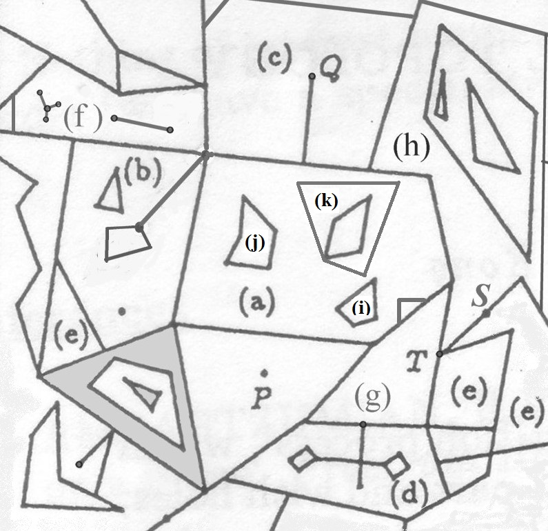
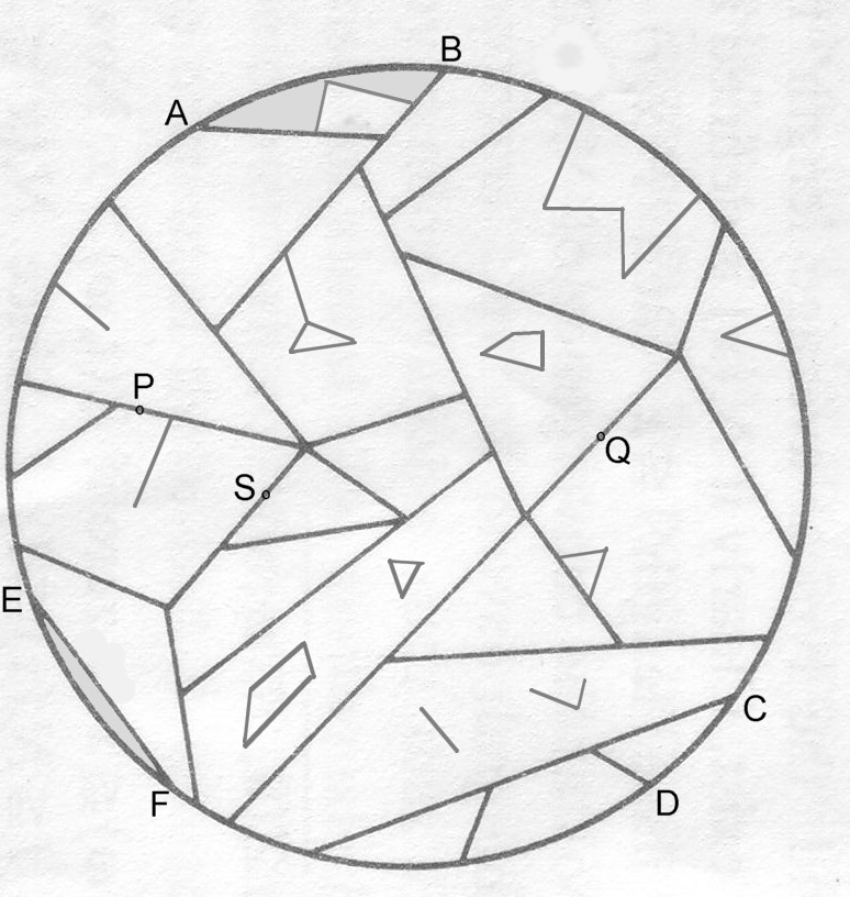
Figure 1 illustrates the graph structure; in particular, the figure shows how complicated the graph’s faces have become. Indeed the definition of a face now requires considerable care.

Figure 1: An infinite geometric graph, as seen within a window. It can also be viewed as a new sort of tessellation having fairly general cells and some status given to a few cell-unions. Using the node, link and face terminology of graph theory, we see that $P$ is a node of valency $0$, whilst $\mathcal{Q}$ is a node of valency $1$. There are many $2$-valent nodes, mostly with non-collinear links emanating; node $S$ is a $2$-valent example with collinear links; it is called a double-$\pi$ node. Node $T$ is one of the many $\pi$-nodes. Viewing the figure as a tessellation, the three cells marked (e) form a cell-union and the two cells shaded a darker grey are the parts of a cell-union; such unions would need to be based on a natural nexus (though the reader won’t see any natural nexus in these two cases). The three cells (i), (j) and (k) have a natural nexus, however, each being cellular holes in the same cell (namely (a)). So we might like to consider (i), (j) and (k) as a cell-union. The text below explains why cell-unions are studied. Cell (a), with three holes, has Euler Entity $-2$. Cell (f) has two holes (each of area zero) comprising three edges and one edge respectively. Other features are discussed in the text.

The concept of a face: In the following definition, the boundary of a set $F\subset\mathrm{R}^{2}$ is defined to be $cl(F)\,\cap\,cl(\bar{F})$, where $cl(\cdot)$ indicates closure and $\bar{F}$ is the complement of $F$. The interior of $F$ is written $int(F)$.

Definition 4

: Let $\mathcal{G}$ be our infinite geometric planar graph defined by its collection of nodes and links. Let $\mathcal{G}_{\cup}$, called the graph-union, be the subset of $\mathrm{R}^{2}$ defined as the union of all nodes and links. An open subset $F$ of $\mathrm{R}^{2}$ is called a face of the graph $\mathcal{G}$ if and only if $F$ is connected, $F\cap\mathcal{G}_{\cup}=\emptyset$ and the boundary of $F$ is contained in $\mathcal{G}_{\cup}$. Subsets $F$ which are not open are not faces.

Assumption: We assume that $\mathcal{G}$ is such that $\mathcal{G}_{\cup}$ has no unbounded faces. We also assume that $\mathcal{G}_{\cup}$ is locally finite: that is, every bounded domain of $\mathrm{R}^{2}$ intersects a finite number of faces.

Our decision to treat each face as an open set deserves comment, because the reader will notice that the occasional face — for example, (a), (g), (h), (i) and (j) in Figure 1 — can be considered as a closed set without changing the graph-union in any way. Many faces, however, have a closure which destroys part of the face’s boundary (and part of the graph-union too) and this significantly alters the face’s topological status. See for example faces (b), (c), (d), (f), (k) and the open ‘quadrilateral with a hole’ that surrounds the isolated node $P$. Also, the open faces (d) and (k) are simply-connected, but their closures are not – and open cell (b) has one hole, its closure two. So certain features of faces naturally occurring in a graph-union would disappear if cells were considered as closed sets. It is important therefore to have a theory based on open faces; thereby greater diversity in the graph-union occurs.

Remark 2

: Modern definitions of a graph face when the graph $\mathcal{G}$ is planar and infinite, but not connected, are rare. Beineke’s [3] definition, which wins for brevity, is as follows. Maximal connected sets in the planar set $\mathrm{R}^{2}\setminus\mathcal{G}_{\cup}$ are called faces. We have not adopted his definition. It would be equivalent to Definition 4, however, if it commenced Maximal connected open sets ....

The generalised tessellation: We started this paper with a traditional convex-celled tessellation of the plane, then transferred our thoughts to its associated geometric planar graph. Then we allowed the graph to have more of the features that geometric graphs can have. Now, as suggested above, we reverse the transfer and look at the planar tessellation–like structure generated by the more elaborate graph. Words such as ‘node’, ‘link’, ‘face’ and ‘graph-union’ return to the more familiar ‘vertex’, ‘edge’, ‘cell’ and ‘frame’ in a tessellation context. Whilst we might still call this structure a tessellation (albeit described as a generalised tessellation or a tessellation derived from a geometric graph), we also call it a planar partitioning.

Both the graph $\mathcal{G}$ and its derived generalised tessellation have a new concept not evident in the convex-celled theory: the double-$\pi$ node or double-$\pi$ vertex.

Definition 5

: A node in $\mathcal{G}$ is called a double-$\pi$ node if, when marked on $\mathcal{G}_{\cup}$, it is $2$-valent with collinear edges emanating. In other words, a node is a double-$\pi$ node if and only if it is a $\pi$-node of valency two. Here, a $\pi$-node is a node with at least one angle formed by consecutive emanating links equal to $\pi$ — and if the valency is two, there are two such angles, so the node is ‘double-$\pi$. A vertex in the derived tessellation is a double-$\pi$ vertex if, in the graph context, it is a double-$\pi$ node — and it is a $\pi$-vertex if it is a $\pi$-node.

Node $S$ in Figure 1 is an example of a double-$\pi$ node; it is, of course, a double-$\pi$ vertex in the tessellation context.

Remark 3

: Does the graph-union $\mathcal{G}_{\cup}$ contain all the information that the graph $\mathcal{G}$ has? No, not unless we make sure that the double-$\pi$ vertices are specially marked, as mentioned in our phrasing of Definition 5. Without marking, these vertices are visually lost in drawings. Therefore, we make a special notation $\mathcal{G}_{\cup}^{+}$ to indicate the ‘marked infinite graph-union’: namely $\mathcal{G}_{\cup}$ with all the double-$\pi$ vertices marked. Although the information in $\mathcal{G}$ is the same as that in $\mathcal{G}_{\cup}^{+}$, we refer to $\mathcal{G}$ as the graph and $\mathcal{G}_{\cup}^{+}$ as the generalised tessellation (or planar partitioning or tessellation derived from $\mathcal{G}$). Any statement in the sequel for $\mathcal{G}$ holds also for $\mathcal{G}_{\cup}^{+}$, but not necessarily for the unmarked $\mathcal{G}_{\cup}$.

Definition 6

: A cell-union of a tessellation derived from a graph is a finite union of some cells of the tessellation.

For example, we have marked a three-celled cell-union (e) in Figure 1. We note again the usefulness of an open-cell theory; the three cells involved in (e) are assumed open sets. Their union comprises three cells, each being a connected set; if we treated cells as closed sets, the union would comprises only two connected parts.

Discussion: By this process of generalisation, we allow planar partitionings which have disconnected features (see Figure 1 and its caption). A cell, though still bounded and connected, might not be simply-connected (that is, it might have ‘holes’). The frame might not be connected; this will be the case if a cell has another cell or cluster of cells wholly enclosed within its interior; the edges of the enclosed cell(s) will be disconnected from most other edges of the graph. Additionally we allow the existence of vertices of valency 1 or 0, the latter type being simply isolated points. The edges are closed line-segments, however, as before.

Perhaps most importantly there are many violations of the rules used by Zähle et. al. All cells are open, therefore not compact. The vertex $P$ contradicts their Rule 4. Cell (a) is not simply-connected, and so on! In short, the rules of Zähle et al, when still meaningful with cells so general, are often violated. Put simply, our planar-partitioning structures are not cell complexes.

3. Counting cell sides, corners, edges and vertices

Sides and corners of cells: There is a need to define a side and a corner of these unusual cells. Our definition involves the concept of a walk on the graph $\mathcal{G}$.

Definition 7

: Consider a sequence of $n\geq 3$ nodes from $\mathcal{G}$ such that consecutive nodes in the sequence have a link between them. A walk on $\mathcal{G}$ is such a sequence beginning and ending with the same node (which we call the walk’s home), without containing home again in the sequence.

For example, if we have nodes labelled $1,2,3$ and $4$ with non-directional links $\{1,3\}$, $\{2,3\},\{2,4\}$ and $\{3,4\}$, then the sequence $w_{1}=(1,3,2,4,3,2,3,1)$ is a walk whose home is $1$.

So a walk contains its home node exactly twice and may contain the other nodes in the sequence more than once. A walk may equivalently be thought of as a journey on $\mathcal{G}_{\cup}^{+}$, visiting the nodes (and the implied connecting links) in the order given by the sequence — a journey that always returns to its starting node, home. In the example, note that $w_{2}=(4,3,2,3,1,3,2,4)$ is a walk, different from $w_{1}$, despite $w_{1}$ and $w_{2}$ having journeys that visit the same nodes in the same ‘cyclic order’.

Definition 8

: A first-exit walk is defined as a walk which ‘exits’ each node visited (except home) on the link which gives the walker the maximum anti-clockwise turn of his body — but if no link involves an anti-clockwise turn, he makes the minimum clockwise turn. If the node is of valency $1$, then the walker makes a clockwise turn of $\pi$ and exits the node back along his entry link. The turning angle is denoted by $\zeta$ and it lies in the range $[-\pi,\pi)$ where anti-clockwise is deemed positive and clockwise negative. An angle $\zeta=0$ applies if the walker doesn’t turn at all. At the conclusion of a first-exit walk, returning to home, it is assumed that the walker turns to face his starting direction. So this last turning angle is assumed to be part of a first-exit walk.

For example entering node $T$ from above, the walker exits along the edge leading to node $S$. Since $S$ has valency $2$, its exit is by the ‘straight-ahead’ link (the only link available). Approaching the $1$-valent node $Q$ from below, the first exit is back along the link of entry, so $\zeta=-\pi$.

Definition 9

:  Let $F$ be a face of $\mathcal{G}$; by assumption $F$ is bounded. A first-exit walk where every node and link in the walk’s sequence lies on the boundary of $F$ and where, when traversing every link of the walk, there is always an open neighbourhood of the walker left of the link and contained in the interior of $F$, is called a face-circuit. There may be more than one face-circuit of the face $F$. The link-count of a face-circuit is the number of link-traversals (so a link traversed twice scores $2$). The node-count of a face-circuit is the number of node-visits made in the face-circuit, counting node home only once. A face-circuit also has a corner-count defined as the number of direction changes in the face-circuit (that is, the number of non-zero turning angles $\zeta$, the nodes in the face-circuit where $\zeta\neq 0$ being called corners of the face circuit). The line-segments in the face-circuit between consecutive corners are called sides of the face circuit; so the face-circuit also has a side-count.

These definitions, defined above for face-circuits, apply also to faces.

Definition 10

:  The corners of a face $F$ are the corners on all $F$’s face-circuits, so the corner-count of a face is the sum of the corner-counts of all face-circuits. Likewise for sides of a face and side-counts of a face and also link-counts of a face. The node-count of a face, however, is the sum of the node-counts for the component face-circuits plus the number of $0$-valent nodes that form holes in the face.

For example, face (a) has four face-circuits with link-counts $10,5,4$ and $4$ and side-counts $8,5,4$ and $4$, so face (a) itself has link-count $23$ and side-count $21$. Face (b) has two face-circuits with link-counts $11$ and $3$, so face (b) has link-count $14$. Faces (c) and (d) each have just one face-circuit with link-counts $9$ and $24$ respectively. Face (f) has an ‘outer’ face-circuit with $7$ link-counts (but only $6$ side-counts) and two ‘inner’ face-circuits with $2$ and $6$ link-counts.

Note that for three of the four face-circuits of (a), the travel direction of the circuit is clockwise (as face (a) must be on the left). For any of the three faces (i), (j) and (k) which make a hole in (a), the face-circuits are travelled anti-clockwise (keeping the ‘hole-cell’ to the left).

Clearly a face-circuit’s node-count always equals its link-count. Its side-count always equals its corner-count.

The word ‘cell’ replaces ’face’ when our discussion turns to generalised tessellations.

Definition 11

: In the generalised tessellation induced by $\mathcal{G}$, a cell is equivalent to a face of $\mathcal{G}$ and a cell-circuit is equivalent to a face-circuit. So the entities edge-count of a cell, side-count of a cell, corner-count of a cell are essentially defined in Definitions 9 and 10. The vertex-count of a cell follows the definition of the node-count of a face in those definitions.

Remark 4

: A concept of a $\pi$-vertex (and double-$\pi$ vertex) can be defined using face-sides. A vertex that lies in at least one face-side interior is called a $\pi$-vertex. A vertex that lies in two face-side interiors is called a double-$\pi$ vertex.

4. Descriptor of the cell’s topology

The topology of a cell is summarised by a functional rather like the Euler Characteristic $\chi$, defined loosely as the number of parts minus the number of ‘holes’. We call this functional, which we define in this section, by different terminology: the Euler Entity. We use a different name because some readers of our theory have remarked that the Euler Characteristic is not usually defined on open sets — and our theory produces cells which are open sets. So the statistical properties of the ‘typical’ cell include mean values of topological features such as $\chi$ and also, of course, geometric features such as area and perimeter plus various combinatorial entities.

Introduction of $\chi$: There are many different contexts in the topological literature where the Euler Characteristic is defined for a set $F\subset\mathrm{R}^{2}$. Mostly, for a valid definition, the set needs to be closed; for example, in some theories $F$ should be in the convex ring. Even in the Gauss-Bonnet context, the usual discourse assumes that $F$ contains its boundary. Our method is essentially of Gauss-Bonnet style, but $F$ is now open; so $F$ doesn’t contain (or even intersect) its boundary.

Figure 2: The grey domain here is an open face with a side-count of $19$. Its boundary is shown in black. We begin a walk on this boundary at home, visiting nodes $A,B,C,B$ again, $E,F,A$ again, $H,...$, keeping the ‘grey face at the left’ rule as links are traversed. Turning angles at some of the nodes visited — $A,C,B,E,F,H$ and $R$ — are shown by red or blue arrows, blue indicating a negative turning angle. Corner $A$ is visited twice but we only show the first visit’s turning angle. Only the arrow of the second visit to $B$ and to $R$ is shown.

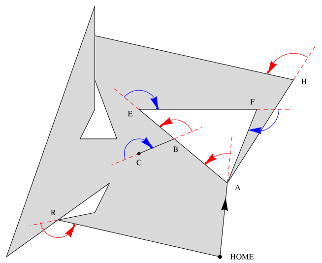
We base the idea on the ‘turning angles’ in $F$’s face-circuits (see Figure 2). As explained above, at each node visit of a face-circuit the walker turns through an anti-clockwise angle $\zeta\in[-\pi,\pi)$ before exiting the node along the ‘first-exit link’. An angle $\zeta=0$ applies if the walker doesn’t turn at all and, in general, $\zeta$ is measured from this ‘collinear entry and exit edges’ situation. By assumption, an anti-clockwise turn gives a positive angle $\zeta\in(0,\pi)$ whilst a clockwise turn (which only occurs if no exit link involving an anti-clockwise turn is available) yields a negative $\zeta\in[-\pi,0)$.

For example when $F$ in Figure 1 is face (h), the walker arriving at $T$ from above turns an angle $\zeta$ of approximately $+140^{\circ}$ (to now walk toward $S$). When $F$ is face (c), arriving at $Q$ from below the walker turns clockwise $180^{\circ}$, so the turning angle is $\zeta=-\pi$. For an arrival at $S$, $\zeta=0$. When $F$ is face (g), an arrival at $T$ from below has $\zeta=0$.

The following lemma, illustrated in Figure 2, is trivially true.

Lemma 1

: For a face-circuit in our geometric graph $\mathcal{G}$ (or for a cell-circuit in the planar partitioning $\mathcal{G}_{\cup}^{+}$), the sum of all turning angles is $2\pi$ if the circuit is anti-clockwise, as in Figure 2. This sum is $-2\pi$ if the circuit is clockwise. $\square$

Thus we are led, in the spirit of the Gauss-Bonnet calculations (see Santaló, [16], p.112), to the following definition.

Definition 12

: In the graph $\mathcal{G}$, the Euler Entity $\chi$ of a face $F$ is defined as the total (over all $F$’s face-circuits) of the turning-angle sums divided by $2\pi$, minus the number of isolated vertices of valency zero in $F$’s interior. In the planar partitioning induced by the graph $\mathcal{G}$, the Euler Entity $\chi$ of a cell is the Euler Entity of the face in $\mathcal{G}$ from which the cell is derived. The Euler Entity $\chi$ of a cell-union is the sum of the Euler Entities for the cells in the union.

Thus the cell in Figure 1 surrounding the $0$-valent vertex $P$ has $\chi=0$. Cells (a), (b), (c), (d), (f) and (h) have Euler Entities $-2,-1,1,1,-1$ and $0$ respectively. Cell-union (e) has $\chi=3$ provided the truncated right-most cell of this cell-union has no holes outside the window. The grey cell-union with one hole has $\chi=1$.

Importantly, one must not interpret the face in Figure 2 as having three holes. It has no holes; the only face-circuit in this face $F$ covers all of $F$’s boundary. Hence the domain has Euler Entity $\chi=1$.

Sample results: In this paper we provide natural generalisations for many of the geometric and topological formulae given in the traditional theory cited in Section 1. The Euler Entity plays an important role. For example if, for the typical cell in a random planar partitioning (RPP) derived from a stationary ergodic random geometric graph, $\mu_{\chi}$ is the expected Euler Entity, $\mu_{E}$ and $\mu_{S}$ are the cell’s expected edge-count and expected side-count whilst, for a typical vertex, $\theta$ is the expected valency and $\phi$ is the expected number of cell-side interiors containing the vertex, then we show that

$$\mu_{E}=\frac{2\theta\mu_{\chi}}{\theta-2}\quad\text{ and }\quad\mu_{S}=\frac{2(\theta-\phi)\mu_{\chi}}{\theta-2},$$ (1)

provided $\theta\neq 2$. We further prove that $\theta=2$ if and only if $\mu_{\chi}=0$. The formulae can also be adapted to studies of cell-unions.

Remark 5

: Consider a tessellation comprising a lattice of regular hexagons with a vertex of valency $0$ placed at the centre of each hexagon, the whole structure being made stationary by randomising the planar origin within one hexagon. It provides an example of a generalised tessellation having $\theta=2$. Note that, because each cell has one hole, then $\mu_{\chi}=0$. Another example with $\theta=2$ and $\mu_{\chi}=0$ arises if each $0$-valent vertex in the example above is replaced by a short closed line-segment that does not hit any hexagon boundary. The ends of the line-segment produce two $1$-valent vertices.

Method: A key tool in our proofs of these and other similar results, is the ergodic method described in [4]-[6] together with the following simple generalisation of Euler’s planar graph identity.

Lemma 2

: Consider a finite (not necessarily connected) planar graph $\mathbf{G}$ having $n$ nodes and $\ell$ links. We assume also that $\mathbf{G}$’s bounded faces has faces have a defined Euler Entity. Let $\mathcal{X}$ be the sum of Euler Entities over all bounded faces. Then,

$$n-\ell+\mathcal{X}=1.$$ (2)

When the graph $\mathbf{G}$ is connected, all bounded faces have $\chi=1$ and so then $\mathcal{X}$ = the number of bounded faces $f$. The familiar form of Euler’s identity is $n-\ell+f=1$, often written as $n-\ell+f^{*}=2$ where $f^{*}=f+1$, counting the unbounded face too. $\square$

The proof is by induction on $\ell$, commencing with any case where $\mathbf{G}$ is connected.

5. Motivating examples

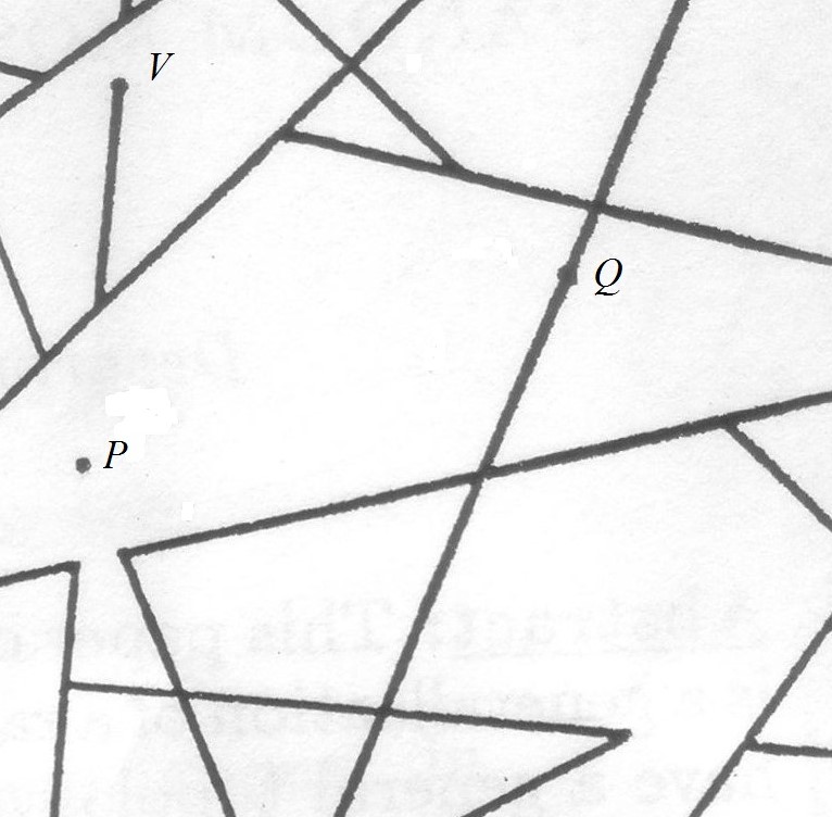
Random deletion of edge interiors: Any tessellation, even one of the traditional kind, may be altered by random edge deletions, each edge interior being deleted independently with probability $q$. Provided $p:=1-q$ is not too small, the result of the deletions provides the frame of a generalised tessellation, including the possible creation of a 0-vertex (see $P$ in Figure 3(a)). From this frame the open tessellation-cells can be constructed. The figure, based on an initial stationary and isotropic Poisson line-process, shows a $1$-vertex (see $V$), four $2$-vertices (one of these, $Q$, being of the collinear double-$\pi$ form) and numerous $\pi$-vertices.

We have not yet investigated the critical value of $p$ for such line processes, below which the cells become unbounded. Readers will note that this structure is similar to structures studied in percolation theory where, in some cases, the critical value of $p$ is known. It will also be noted that sometimes the percolation problem is cast as a random addition of links to a stationary point process of nodes that initially has no links.

(a)                                                                                      (b)

Figure 3: (a) A tessellation formed by a random line process with the random deletion of edge interiors. Here $P$ is a $0$-valency vertex caused by the chance deletion of all its emanating edge-interiors. (b) A realisation of a falling-leaf tessellation with variation in the size and shape of the rectangular leaves.

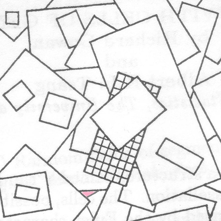
Falling leaf model: When opaque leaves fall randomly on the plane [8], those falling later will cover the others below. Under assumptions of stationarity of leaves, the uncovered leaf-boundaries will form a RPP. The case of leaves congruent to a given simple polygon, where no leaf fits inside another, was studied in [8]. With variation in size and shape of leaves, however, cells of the tessellation may have other cells wholly enclosed. So we have examples of the ‘holes’ in cells (see Figure 3(b) where the falling leaves are rectangles, assumed closed).

This model also provides a motivation for introducing cell-unions. The hatched domain in Figure 3(b), comprises three disconnected cells. There is a clear nexus between these pieces; they all belong to the same fallen leaf but have become disconnected by the position(s) of a later leaf (or leaves). Perhaps one could declare that these cells be grouped as a cell-union. If so, $\chi=3$ for the particular cell-union.

Another aspect of this falling-leaf tessellation is the emergence of some closed cells, some open cells and some ‘neither open nor closed’ cells. This occurs because if a closed leaf $L_{1}$ is first hit by a closed leaf $L_{2}$, without the boundary of $L_{1}$ being covered by $L_{2}$, then the visible part of $L_{1}$ is now $L_{1}\setminus L_{2}$ (and this is not open). In general, the visual part of a leaf whose boundary is partly covered, is neither open nor closed. Yet in other situations, the visual part may be open or closed. A cell (shaded pink) belonging to a leaf whose boundary has been completely covered is an open set. Recently-fallen closed leaves not yet hit by any later leaf are closed sets. So, in order to conform to our theory, we need to focus on the new tessellation frame at the time of observation and construct open cells only from the frame (not a mix of topological types from the physical process of leaf-coverage). The falling leaf model also has many vertices of valency two and many $\pi$-vertices.

Tilings beyond the theory of Grünbaum and Shephard: In Figure 4 are two tilings that have periodic repetition, via translation of a sub-collection of the tiles. These tilings violate the basic assumption N.1 of Grünbaum and Shephard [11] (which states that all tiles must be isomorphic to a closed disk). Although the cells in Figure 4(a) might be considered closed, doing so would lead to a violation of the assumption N.2 of these authors (the intersection of any two tiles is a connected set); see page 121 of their book for these assumptions. With Figure 4(b), one of the cells cannot be considered closed as this operation destroys a tessellation edge. We, of course, consider all cells in both figures as open sets.

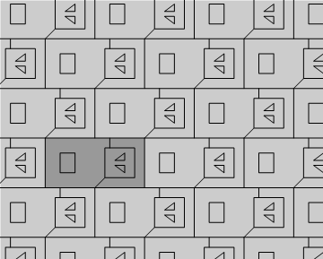
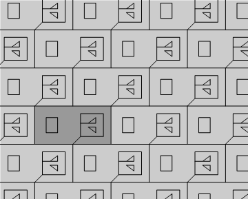
(a)                                                                                      (b)

Figure 4: Two periodic tilings based, in each case, on the darkly shaded sub-collection of tiles (which occupy a rectangle of dimension $2\times 1)$ units. We assume the origin is uniformly distributed inside this rectangle, thereby making each tiling/tessellation stationary.

Our results bring some quantitative tools to these non-traditional tilings. For the example in Figure 4(a), consider the six open cells in the darkly shaded rectangle viewed as follows:

• a small rectangle (side-count $S=4$, edge-count $E=4$, Euler Entity $\mathcal{X}=1$);

• a heptagon with the above rectangle as a hole ($S=11$, $E=13$, $\mathcal{X}=0$);

• two triangles (each has $S=3$, $E=3$, $\mathcal{X}=1$);

• the rectangle which has the triangles as holes ($S=10$, $E=11$, $\mathcal{X}=-1$);

• the octagon ($S=8$, $E=8$, $\mathcal{X}=1$).

So, by direct calculation, $\mu_{S}=(4+11+3+3+10+8)/6=\tfrac{13}{2}$, $\mu_{E}=(4+13+3+3+11+8)/6=7$ and $\mu_{\chi}=(1+0+1+1-1+1)/6=\tfrac{1}{2}$. Or, we might first observe that $18$ vertices are associated with the dark rectangle: the $15$ inside and the three left-most vertices on its boundary (we can’t count all the boundary vertices as this would introduce much double counting across the tessellation). From these $18$ vertices we calculate that $\theta=\tfrac{7}{3}$ and $\phi=\tfrac{1}{6}$. Thus, from our new formulae in (1),

$$\mu_{E}=\frac{2\times\tfrac{7}{3}\times\tfrac{1}{2}}{\tfrac{7}{3}-2}=7\quad\text{ and }\quad\mu_{S}=\frac{2\times(\tfrac{7}{3}-\tfrac{1}{6})\times\tfrac{1}{2}}{\tfrac{7}{3}-2}=\frac{13}{2}.$$

Thus the directly calculated values are in accord with the formulae of our new theory shown in (1). Analysis of Figure 4(b) is left as an exercise for the reader.

6. Theoretical framework

Our generalised theory can follow [6] to some extent, though initially we assume that no cell-unions in the structure are of interest; thus we are only interested in cells. As in Section 1, we let $(\Omega,\mathcal{Q},\mathbb{P})$ be a probability field, where $\Omega$ is the set of all allowed infinite structures $\mathcal{G}_{\cup}^{+}$ that are derived from an infinite geometric graph $\mathcal{G}$. $\mathcal{Q}$ is a $\sigma$-algebra containing all the events of interest to us. The element $\omega\in\Omega$ is one realisation of $\mathcal{G}_{\cup}^{+}$. So $(\Omega,\mathcal{Q},\mathbb{P})$ is our random partition process. For $x,\ t\in\mathrm{R}^{2}$ define the translation operator $T^{t}:x\rightarrow x+t$. Thus $T^{t}$, defined on $\Omega$, translates any realisation $\omega$ by $t$. As in Section 1, we assume that the process is stationary and ergodic, via the assumption that $T^{t}$ (now defined on $\mathcal{Q}$) is a measure-preserving and ergodic operator.

An important consequence of ergodicity is Wiener’s ergodic theorem [4, 6], which states that, if $X$ is any random variable derived from the RPP such that $\mathbb{E}|X|<\infty$ and $B_{r}$ is the closed ball of radius $r$, centre 0 in $\mathrm{R}^{2}$, then for almost all $\omega$

$$\lim_{r\rightarrow\infty}\frac{1}{\pi r^{2}}\int_{B_{r}}X(T^{t}\omega)dt=\mathbb{E}(X).$$ (3)

Let $D$ be any compact convex reference domain in $\mathrm{R}^{2}$ unrelated to our RPP. In $D$, the ‘entire’ edges or cells are those wholly in $D$; the other edges and other cells that intersect $D$ are called ’truncated’. An ‘edge-part’ or ‘cell-part’ in $D$ refers respectively to any entire or truncated edge or cell. A cell ’centre’ is any convenient reference point of the cell, for example the cell’s centroid. Define

$$N(D):=\ D$$ the number of cell-parts in ,

$$N^{\prime}(D):=\ D$$ the number of entire cells in ,

$$n_{\text{cells}}(D):=\ D$$ the number of cell centres in ,

$$\ell(D):=\ D$$ the total length of edge-segments in ,

$$M(D):=\ D$$ the number of edge-parts in ,

$$M^{\prime}(D):=\ D$$ the number of entire edges in ,

$$M^{\partial}(D):=\ \partial D$$ the number of hittings of by edges,

$$n_{\text{verts[k]}}(D):=\ D k$$ the number of vertices within of valency ,

$$n_{\text{edges}}(D):=\ D$$ the number of edge mid-points in ,

$$n_{\text{edges}}^{*}(D):=\ D$$ the number of edge ends in ,

$$n_{\text{$\pi$-verts[k]}}(D):=\ \pi D k$$ the number of -vertices in of valency .

Note that a common symbol, a subscripted $n$, is used for counts of ‘points’ (where the points might be vertices, cell centroids, edge mid-points or edge ends). The subscript indicates the type of point.

Where there is a need to emphasise the dependence on the realisation $\omega$, we use the extended notation, $\ell(D,\omega)$ say. It can be shown, by some elementary inequalities mostly given in [6], that the assumptions $\mathbb{E}M(D)<\infty$ and $\mathbb{E}n_{\text{verts[0]}}(D)<\infty$ are sufficient to ensure that all these quantities have finite expectation for bounded $D$. We make these assumptions and also assume that $\mathbb{E}M(D)>0$ if $|D|$, the Lebesgue measure of $D$, is positive. Note that

$$n_{\text{edges}}^{*}(D)=\sum k\ n_{\text{verts[k]}}(D).$$ (4)

This summation, and all summations in the remainder of this paper, are for $k\geq 0$, unless otherwise marked.

Under stationarity, $\mathbb{E}\ell(\cdot),\mathbb{E}n_{\text{cells}}(\cdot),\mathbb{E}n_{\text{edges}}(\cdot),\mathbb{E}n_{\text{verts[k]}}(\cdot)$ and $\mathbb{E}n_{\text{$\pi$-verts[k]}}(\cdot)$ are measures, proportional to Lebesgue measure. So we may introduce the finite constants $\alpha,\lambda_{\text{cells}},\lambda_{edges},\lambda_{\text{verts}[k]}$ and $\lambda_{\text{$\pi$-verts}[k]},\ (k\geq 0)$ such that

$$\mathbb{E}n_{\text{cells}}(D)=\ \lambda_{\text{cells}}|D|\qquad\quad \mathbb{E}\ell(D)=\ \alpha|D|$$

$$\mathbb{E}n_{\text{edges}}(D)=\ \lambda_{\text{edges}}|D|\qquad\quad \mathbb{E}n_{\text{verts[k]}}(D)=\ \lambda_{\text{verts}[k]}|D|$$

$$\mathbb{E}n_{\text{$\pi$-verts[k]}}(D)=\ \lambda_{\text{$\pi$-verts}[k]}|D|.$$

These parameters, except $\alpha$, are the intensities of stationary point processes in $\mathrm{R}^{2}$. We see from (4) that $\mathbb{E}n_{\text{edges}}^{*}(\cdot)$ is also a measure with $\mathbb{E}n_{\text{edges}}^{*}(D)=\sum k\ \lambda_{\text{verts}[k]}|D|$. Note that $\alpha>0$ and $\lambda_{\text{$\pi$-verts}[0]}=\lambda_{\text{$\pi$-verts}[1]}=0$. We also assume that $\lambda_{\text{cells}}$, $\lambda_{\text{edges}}$, $\lambda_{\text{verts}}:=\sum\lambda_{\text{verts}[k]}$ and $\lambda_{\text{$\pi$-verts}}:=\sum\lambda_{\text{$\pi$-verts}[k]}$ are positive.

7. Ergodic theory

If $D$ is taken to be the ball $B_{r}$, ergodic arguments can now be applied to show that, for example, $\ell(B_{r})/\pi r^{2}\rightarrow\alpha$ almost surely as $r\rightarrow\infty$. To understand the detailed use of (3), take $B_{r}$ and $B_{y},\ y\ll r$, and consider a random variable, associated with $B_{y}$. Then consider this random variable for the translated disk $T^{-t}B_{y}$ and integrate over all $t$, firstly within $B_{r-y}$ and then within $B_{r+y}$. For example, consider the two integrals

$$I_{1}=\int_{B_{r-y}}n_{\text{verts[k]}}(T^{-t}B_{y},\omega)dt,\qquad I_{2}=\int_{B_{r+y}}n_{\text{verts[k]}}(T^{-t}B_{y},\omega)dt.$$

If we now draw a circle of radius $y$ around each $k$-vertex and consider the sum of these circular areas (including any parts which may extend beyond $B_{r}$) then this sum, which is obviously equal to $\pi y^{2}n_{\text{verts[k]}}(B_{r},\omega)$, is bounded below by $I_{1}$ and above by $I_{2}$. Noting that $n_{\text{verts[k]}}(T^{-t}B_{y},\omega)=n_{\text{verts[k]}}(B_{y},T^{t}\omega)$, we have that

$$\int_{B_{r-y}}n_{\text{verts[k]}}(B_{y},T^{t}\omega)dt\leqq\pi y^{2}n_{\text{verts[k]}}(B_{r},\omega)\leqq\int_{B_{r+y}}n_{\text{verts[k]}}(B_{y},T^{t}\omega)dt.$$

Therefore

$$\frac{\pi(r-y)^{2}}{\pi r^{2}}\int_{B_{r-y}}\frac{n_{\text{verts[k]}}(B_{y},T^{t}\omega)}{\pi(r-y)^{2}}dt\leqq\frac{\pi y^{2}n_{\text{verts[k]}}(B_{r},\omega)}{\pi r^{2}}\leqq\frac{\pi(r+y)^{2}}{\pi r^{2}}\int_{B_{r+y}}\frac{n_{\text{verts[k]}}(B_{y},T^{t}\omega)}{\pi(r+y)^{2}}dt.$$

The left and right sides of this inequality converge with probability one to the same quantity, $\mathbb{E}n_{\text{verts[k]}}(B_{y})$, by applying the Wiener ergodic theorem (3). Therefore

$$\frac{n_{\text{verts[k]}}(B_{r},\omega)}{\pi r^{2}}\overset{\text{a.s.}}{\longrightarrow}\frac{\mathbb{E}n_{\text{verts[k]}}(B_{y})}{\pi y^{2}}=\lambda_{\text{verts}[k]}.$$ (5)

With an almost identical argument one can show that the other counting variates associated with point processes converge almost surely.

$$\frac{n_{\text{$\pi$-verts[k]}}(B_{r},\omega)}{\pi r^{2}}\overset{\text{a.s.}}{\longrightarrow}\frac{\mathbb{E}n_{\text{$\pi$-verts[k]}}(B_{y})}{\pi y^{2}}=\ \lambda_{\text{$\pi$-verts}[k]},$$ (6)

$$\frac{n_{\text{edges}}B_{r},\omega)}{\pi r^{2}}\overset{\text{a.s.}}{\longrightarrow}\frac{\mathbb{E}n_{\text{edges}}B_{y})}{\pi y^{2}}=\ \lambda_{\text{edges}},$$ (7)

$$\frac{n_{\text{cells}}(B_{r},\omega)}{\pi r^{2}}\overset{\text{a.s.}}{\longrightarrow}\frac{\mathbb{E}n_{\text{cells}}(B_{y})}{\pi y^{2}}=\ \lambda_{\text{cells}},$$ (8)

whilst from (4) and (5)

$$\frac{n_{\text{edges}}^{*}B_{r},\omega)}{\pi r^{2}}\overset{\text{a.s.}}{\longrightarrow}\frac{\mathbb{E}n_{\text{edges}}^{*}B_{y})}{\pi y^{2}}=\sum k\ \lambda_{\text{verts}[k]}.$$ (9)

If the quantity $\ell(B_{y},\omega)$ is integrated in the same manner we obtain the inequality

$$\int_{B_{r-y}}\ell(B_{y},T^{t}\omega)dt\leq\pi y^{2}\ell(B_{r},\omega)\leq\int_{B_{r+y}}\ell(B_{y},T^{t}\omega)dt.$$

Here, the middle expression involves a small calculation. Around each segment in $B_{r}$, construct a sausage-shaped domain of points within distance $y$ of that segment. As the centre of a disk $B_{y}$ moves over all positions within the domain, it can easily be shown that an integration of the segment length within $B_{y}$ yields $\pi y^{2}$ times the segment length. Adding over all ‘sausage’ domains yields $\pi y^{2}\ell(B_{r},\omega)$. Dividing by $\pi r^{2}$, taking limits and applying the Wiener ergodic theorem proves that

$$\frac{\ell(B_{r},\omega)}{\pi r^{2}}\overset{\text{a.s.}}{\longrightarrow}\alpha.$$ (10)

Next we consider the integrals $I_{1}$ and $I_{2}$ (say) of $M(B_{y},T^{t}\omega)$, or equivalently $M(T^{-t}B_{y},\omega)$, as $t$ moves over $B_{r-y}$ and $B_{r+y}$ respectively. These integrals provide lower and upper bounds for the sum of areas for all of the ‘sausage’ domains. This sum is easily seen to be $2y\,\ell(B_{r},\omega)+\pi y^{2}M(B_{r},\omega)$. Thus

$$I_{1}:=\int_{B_{r-y}}M(B_{y},T^{t}\omega)dt\leq 2y\,\ell(B_{r},\omega)+\pi y^{2}M(B_{r},\omega)\leq\int_{B_{r+y}}M(B_{y},T^{t}\omega)dt=:I_{2}.$$

Dividing by $\pi r^{2}$, taking limits and using (3) and (10), shows that

$$\frac{M(B_{r},\omega)}{\pi r^{2}}\overset{\text{a.s.}}{\longrightarrow}\frac{\mathbb{E}M(B_{y})}{\pi y^{2}}-\frac{2\alpha}{\pi y}.$$ (11)

In adding the areas of the ‘sausage’ domains, we included the semi-circular parts which extend beyond $B_{r}$ when an edge hits $\partial B_{r}$. If these semi-circular areas are not counted, we find that

$$I_{1}\leq 2y\,\ell(B_{r},\omega)+\frac{1}{2}\pi y^{2}\sum k\ n_{\text{verts[k]}}(B_{r},\omega)\leq I_{2}.$$ (12)

This is a precise way of saying that, since each edge has two ends, $2M(B_{r})=\sum k\ n_{\text{verts[k]}}(B_{r})$ except for the boundary effects of $\partial B_{r}$. Thus, the middle expression in (12), when divided by $\pi r^{2}$ converges almost surely to $\mathbb{E}M(B_{r})$. We already know however from (5) and (10), that it converges to $2y\alpha+\frac{1}{2}\pi y^{2}\sum k\ \lambda_{\text{verts}[k]}$, so

$$\mathbb{E}M(B_{y})=2y\alpha+\frac{1}{2}\pi y^{2}\sum k\ \lambda_{\text{verts}[k]}.$$ (13)

From (11) and (13), therefore,

$$\frac{M(B_{r})}{\pi r^{2}}\overset{\text{a.s.}}{\longrightarrow}\frac{1}{2}\sum k\ \lambda_{\text{verts}[k]}.$$ (14)

8. Sampling the typical vertex or typical edge

The mean valency of a ‘typical’ vertex of the RPP, denoted by $\theta$, is defined as the limit of the total valency of vertices within $B_{r}$ divided by the number of vertices in $B_{r}$, as $r\rightarrow\infty$, whenever this almost-sure limit exists and yields a constant. We have established existence because, using (5),

$$\theta:=\ \lim_{r\rightarrow\infty}\frac{\sum k\ n_{\text{verts[k]}}(B_{r},\omega)}{\sum n_{\text{verts[k]}}(B_{r},\omega)}$$

$$=\ \frac{\sum k\ \lambda_{\text{verts}[k]}}{\sum\lambda_{\text{verts}[k]}}=\frac{\sum k\ \lambda_{\text{verts}[k]}}{\lambda_{\text{verts}}}$$ (15)

where $\lambda_{\text{verts}}$ is the intensity of the point process of all vertices.

In a similar fashion, the mean length of a ‘typical’ edge of the RPP, denoted by $\nu$, is defined as the limit of total segment length within $B_{r}$, divided by the number of edge-segments in $B_{r}$. Thus, from (10) and (14),

$$\nu:=\ \lim_{r\rightarrow\infty}\frac{\ell(B_{r},\omega)}{M(B_{r},\omega)}$$

$$=\ \frac{2\alpha}{\sum k\ \lambda_{\text{verts}[k]}}=\frac{2\alpha}{\lambda_{\text{verts}}\theta}.$$ (16)

9. Edges hitting the boundary

The edges of our process can be viewed as a stationary line-segment process (LSP) of a general kind. Following [5], we have that for $y>0$

$$M(B_{r})-M^{\prime}(B_{r})\leq[\ell(B_{r+y})-\ell(B_{r})]/y+n_{\text{edges}}^{*}(B_{r+y})-n_{\text{edges}}^{*}(B_{r}).$$

Thus from this inequality, combined with (9) and (10), we see that the normalised number of edges hitting the boundary is almost surely asymptotically negligible as $r\rightarrow\infty$, that is,

$$\frac{M(B_{r})-M^{\prime}(B_{r})}{\pi r^{2}}\overset{\text{a.s.}}{\longrightarrow}0.$$ (17)

Since $M^{\prime}\leq n_{\text{edges}}\leq M$, we see that $n_{\text{edges}}(B_{r})/\pi r^{2}$ and $M(B_{r})/\pi r^{2}$ converge almost surely to the same limit, namely that given in (14). Thus from (7), (14) and (15), $2\lambda_{\text{edges}}=\lambda_{\text{verts}}\theta$, a result which, combined with (16), permits many rearrangements, for example,

$$\lambda_{\text{edges}}=\frac{\alpha}{\nu}.$$ (18)

Note that $M-M^{\prime}=M^{\partial}_{1}+M^{\partial}_{2}$ where $M^{\partial}_{i}$ is defined as the number of edges which cut the boundary $i$ times. Thus $M^{\partial}_{i}(B_{r})/\pi r^{2}\overset{\text{a.s.}}{\longrightarrow}0$ and since $M^{\partial}=M^{\partial}_{1}+2M^{\partial}_{2}$, we see also that $M^{\partial}(B_{r})/\pi r^{2}\overset{\text{a.s.}}{\longrightarrow}0$.

10. Sampling the typical cell

We now focus attention on the random finite graph $\mathbf{G_{r}(\omega)}$ whose nodes and links are as follows.

• The nodes are all vertices of the RPP which lie in $B_{r}$, together with all points where the boundary $\partial B_{r}$ intersects an edge of the RPP.

• The links are all edge-parts in $B_{r}$ together with all the circular arcs which make up $\partial B_{r}$.

Here $\omega$ is the infinite graph realised randomly. Any cell-part formed within $B_{r}$ has an area $A$ and perimeter $L$ (perhaps involving part of $\partial B_{r}$). The sums of area and perimeter over all regions are denoted by $\mathcal{A}(B_{r})$ and $\mathcal{L}(B_{r})$ and it is clear that

$$\mathcal{A}(B_{r})=\ \pi r^{2}\qquad\text{and}\qquad\mathcal{L}(B_{r})=\ 2\ell(B_{r})+2\pi r.$$

The vertex-count $V$, edge-count $E$, side-count $S$ and corner-count $C$ of a cell-part are defined in Definition 11 when the cell-part is an entire cell. Those definitions apply immediately to the truncated cells by simply treating the arcs as links. For example, in Figure 5 the side-count of the two shaded cell-parts are $5$ and $2$, treating the arcs $\mathsf{A}\mathsf{B}$ and $\mathsf{E}\mathsf{F}$ as sides. One can also extend the definition of the Euler Entity to any truncated cell having circular arcs on its boundary; we add an ‘arc turning angle’ which, in the spirit of Gauss-Bonnet, is the total angle turned by the walker when he traverses the arc. It can be expressed as an integral of curvature over the arc even for open sets (see Santaló, [16], formula 7.16).

Figure 5: The finite graph $\mathbf{G}_{r}(\omega)$ comprises the planar partitioning within $B_{r}$ together with $\partial B_{r}$. All double-$\pi$ vertices, those labelled $\mathsf{P},\mathsf{Q}$ and $\mathsf{S}$, are marked. For the entire cells, the Euler Entity, the edge-count, side-count, etcetera, are defined by our earlier definitions. For a truncated cell, which typically has an arc from $\partial B_{r}$ on its boundary, the text describes one how these quantities are calculated. For example, the cell-parts whose arcs are $\mathsf{A}\mathsf{B},\mathsf{C}\mathsf{D}$ or $\mathsf{E}\mathsf{F}$ each have Euler Entity $1$.

Remark 6

: For most of the truncated cells, the Euler Entity can be calculated correctly by first replacing any arc, say $\mathsf{C}\mathsf{D}$, by a line-segment having the same end points. But this device doesn’t work when the truncated cell is like one of the two shaded sets. In these cases, however, one can replace the arc with a polygonal chain — then calculate the Euler Entity using our usual definition for simple polygons. The use of an arc turning angle is the simplest approach, we think.

Sums of the entities vertex-count $V$, edge-count $E$, side-count $S$ and corner-count $C$ over all cell-parts in $B_{r}$ are denoted by $\mathcal{V}(B_{r}),\mathcal{E}(B_{r}),\mathcal{S}(B_{r})$ and $\mathcal{C}(B_{r})$, using script letters. Clearly,

$$\mathcal{E}(B_{r})=\ 4M(B_{r})-\sum k\ n_{\text{verts[k]}}(B_{r})$$

$$\mathcal{C}(B_{r})=\ \mathcal{E}(B_{r})-2n_{\text{$\pi$-verts[2]}}(B_{r})-\sum_{k\geq 3}n_{\text{$\pi$-verts[k]}}(B_{r})$$

$$\mathcal{V}(B_{r})=\ \mathcal{}E(B_{r})+n_{\text{verts[0]}}(B_{r})$$ (19)

$$\mathcal{S}(B_{r})=\ \mathcal{C}(B_{r}).$$

Moreover the sum $\mathcal{X}(B_{r})$ of Euler Entities over all cell-parts can be found from Lemma 2 using the finite graph $\mathbf{G}_{r}(\omega)$. Thus $n=\sum n_{\text{verts[k]}}(B_{r})+M^{\partial}(B_{r}),\ \ell=M(B_{r})+M^{\partial}(B_{r})$ and $\mathcal{X}=\mathcal{X}(B_{r})$, so (2) becomes

$$\mathcal{X}(B_{r})=M(B_{r})-\sum n_{\text{verts[k]}}(B_{r})+1.$$ (20)

We define the mean of a cell-part feature, for example of area $A$, as the limit as $r\rightarrow\infty$ of an appropriate cell-part sum, $\mathcal{}A(B_{r})$ say, divided by the number $N(B_{r})$ of cells, if this ratio converges to a constant almost surely. We denote such mean values by $\mu$, suitably subscripted. Thus

$$\mu_{A}:=\ \lim_{r\rightarrow\infty}\frac{\mathcal{A}(B_{r})}{N(B_{r})}$$

$$\mu_{L}:=\ \lim_{r\rightarrow\infty}\frac{\mathcal{L}(B_{r})}{N(B_{r})}$$

$$\mu_{\chi}:=\ \lim_{r\rightarrow\infty}\frac{\mathcal{X}(B_{r})}{N(B_{r})}$$

$$\mu_{V}:=\ \lim_{r\rightarrow\infty}\frac{\mathcal{V}(B_{r})}{N(B_{r})}$$ (21)

$$\mu_{E}:=\ \lim_{r\rightarrow\infty}\frac{\mathcal{E}(B_{r})}{N(B_{r})}$$

$$\mu_{S}=\mu_{C}:=\ \lim_{r\rightarrow\infty}\frac{\mathcal{C}(B_{r})}{N(B_{r})}$$

whenever the appropriate limit exists almost surely. In [6], these entities were defined as the limit of the expected ratio, for example $\lim\mathbb{E}(\mathcal{A}(B_{r})/N(B_{r}))$, when that limit exists. The definition that we adopt in (21), and earlier in (15) and (16), avoids certain technicalities and is, in all examples that we have experienced, equivalent to that in [6].

Thus we can say, from (5), (6), (10) and (14) that

$$\frac{\mathcal{A}(B_{r})}{\pi r^{2}}\ \overset{\text{a.s.}}{\longrightarrow}1$$

$$\frac{\mathcal{X}(B_{r})}{\pi r^{2}}\ \overset{\text{a.s.}}{\longrightarrow}\frac{1}{2}\sum^{\infty}_{k=0}(k-2)\lambda_{\text{verts}[k]}=\frac{\lambda_{\text{verts}}(\theta-2)}{2}$$

$$\frac{\mathcal{L}(B_{r})}{\pi r^{2}}\ \overset{\text{a.s.}}{\longrightarrow}2\alpha$$

$$\frac{\mathcal{V}(B_{r})}{\pi r^{2}}\ \overset{\text{a.s.}}{\longrightarrow}\lambda_{\text{verts}[0]}+\sum^{\infty}_{k=1}k\ \lambda_{\text{verts}[k]}=\lambda_{\text{verts}}(\theta+\xi)$$ (22)

$$\frac{\mathcal{E}(B_{r})}{\pi r^{2}}\ \overset{\text{a.s.}}{\longrightarrow}\sum^{\infty}_{k=1}k\ \lambda_{\text{verts}[k]}=\lambda_{\text{verts}}\theta$$

$$\frac{\mathcal{S}(B_{r})}{\pi r^{2}}\ \overset{\text{a.s.}}{\longrightarrow}\sum^{\infty}_{k=1}k\ \lambda_{\text{verts}[k]}-\sum^{\infty}_{k=3}\lambda_{\text{$\pi$-verts}[k]}-2\lambda_{\text{$\pi$-verts}[2]}=\lambda_{\text{verts}}(\theta-\phi).$$

Here $\phi$ is the mean number of angles equal to $\pi$ at a ‘typical’ vertex. Formally, $\phi$ is the almost-sure limit

$$\lim_{r\rightarrow\infty}\frac{\sum\limits^{\infty}_{k=3}n_{\text{$\pi$-verts[k]}}(B_{r})+2n_{\text{$\pi$-verts[2]}}(B_{r})}{\sum n_{\text{verts[k]}}(B_{r})}=\frac{\lambda_{\text{$\pi$-verts}}+\lambda_{\text{$\pi$-verts}[2]}}{\lambda_{\text{verts}}}.$$

In addition, $\xi$ is the proportion of vertices which are of valency zero.

These results show that the numerators in (21) converge almost surely to constants, when normalised by $\pi r^{2}$. We now show that $N(B_{r})/\pi r^{2}$ converges likewise, thereby establishing the conditions for the mean features for typical cells to be finite.

11. Asymptotics of $N(B_{r})$

Firstly we need to show that $N(B_{r})-N^{\prime}(B_{r})$, the number of truncated cells, becomes asymptotically negligible relative to $\pi r^{2}$ as $r\rightarrow\infty$. It is a trivial fact that the number of truncated cells is bounded above by $M^{\partial}(B_{r})$. For an ergodic line-segment process it is shown in [5] that, provided the expected number of these line-segments hitting a bounded domain $D$ is finite, the number of crossing points of edges with $\partial B_{r}$, when normalised by $\pi r^{2}$, tends almost surely to zero. Thus in our theory, $M^{\partial}(B_{r})/\pi r^{2}\overset{\text{a.s.}}{\longrightarrow}0$ since we already have the regularity condition $\mathbb{E}M(D)<\infty$. Thus

$$\frac{N(B_{r})-N^{\prime}(B_{r})}{\pi r^{2}}\overset{\text{a.s.}}{\longrightarrow}0.$$ (23)

Let $A_{t}$ be the area of the cell which covers $t\in\mathrm{R}^{2}$ with $A_{t}$ defined as zero if $t$ lies on an edge of the RPP. Stationarity implies that the distribution of $A_{t}$ is independent of $t$. Now, following [6], consider the integral

$$I=\int_{B_{r}}\frac{dt}{A_{t}(\omega)}=\int_{B_{r}}\frac{dt}{A_{0}(T^{-t}\omega)}.$$

This integral is approximately equal to $N(B_{r},\omega)$. Precisely $N^{\prime}(B_{r},\omega)\leq I\leq N(B_{r},\omega)$. Since $N(B_{r})\leq M(B_{r})+1$, $EN(B_{r})<\infty$, so $E(I)$ is finite. Thus from Fubini’s theorem and homogeneity, $E(1/A_{0})$ is finite. Wiener’s theorem can thus be employed to show that $I/\pi r^{2}\overset{\text{a.s.}}{\longrightarrow}E(1/A_{0})$. Rewriting the inequality as $I-(N-N^{\prime})\leq N^{\prime}\leq I$ and noting (23), we establish that $N^{\prime}/\pi r^{2}\overset{\text{a.s.}}{\longrightarrow}E(1/A_{0})$ which, from (23) too, implies that

$$\frac{N(B_{r})}{\pi r^{2}}\overset{\text{a.s.}}{\longrightarrow}E(1/A_{0}).$$ (24)

12. Cellular mean values

We have established that the denominators in (16), normalised by $\pi r^{2}$, converge almost surely to a constant. Thus in conducting the ‘ergodic experiment’ to sample the typical cell, we have proved the finiteness of mean values $\mu_{A},\ \mu_{L},\ \cdots$, defined in (21). In particular

$$\mu_{A}=\lim_{r\rightarrow\infty}\frac{\mathcal{A}(B_{r})/\pi r^{2}}{N(B_{r})/\pi r^{2}}=\frac{1}{E(1/A_{0})}.$$ (25)

Thus the unfamiliar entity $E(1/A_{0})$, which appears in (24), has a convenient evaluation in terms of the mean cell area, namely

$$E(1/A_{0})=1/\mu_{A}.$$ (26)

Further results which follow directly from (21), (22) and (24) are, using (26), (16) and (18),

$$\mu_{L}=\ 2\alpha\mu_{A}=\lambda_{\text{verts}}\theta\nu\mu_{A}=2\lambda_{\text{edges}}\nu\mu_{A}$$

$$\mu_{\chi}=\ \frac{\lambda_{\text{verts}}(\theta-2)\mu_{A}}{2}=(\lambda_{\text{edges}}-\lambda_{\text{verts}})\mu_{A}$$ (27)

$$\mu_{E}=\ \lambda_{\text{verts}}\theta\mu_{A}=2\lambda_{\text{edges}}\mu_{A}$$

$$\mu_{S}=\mu_{C}=\ \lambda_{\text{verts}}(\theta-\phi)\mu_{A}$$

$$\mu_{V}=\ \lambda_{\text{verts}}(\theta+\xi)\mu_{A}$$ (28)

Clearly these formulae permit a large number of rearrangements including the interesting topological-linkage formulae promised in (1).

$$\mu_{E}=\ \frac{2\theta\mu_{\chi}}{\theta-2}$$ (29)

$$\mu_{S}=\mu_{C}=\ \frac{2(\theta-\phi)\mu_{\chi}}{\theta-2}$$ (30)

$$\mu_{V}=\ \frac{2(\theta+\xi)\mu_{\chi}}{\theta-2}$$ (31)

which hold when $\theta\neq 2$.

Using (27), it is readily proved that $\theta=2$ if and only if $\mu_{\chi}=0$, since $\lambda_{\text{verts}}>0$ and $\mu_{A}>0$. Formulae (29)–(31) are interesting generalisations of formulae for the ergodic convex-celled tessellation treated in [4], [6] and [7], where $\mu_{\chi}=1$.

$$\mu_{E}=\ \mu_{V}=\frac{2\theta}{\theta-2}$$ (32)

$$\mu_{S}=\ \mu_{C}=\frac{2(\theta-\phi)}{\theta-2}.$$ (33)

13. Point processes

We have already seen that there is a point process of vertices, intensity $\lambda_{\text{verts}}$, and a point process of edge mid-points, intensity $\lambda_{\text{edges}}$. Cells can be given a reference point, for example the centroid, and these reference locations form a point process, whose intensity we denote by $\lambda_{\text{cells}}$. With all point processes, the count of points within $B_{r}$, divided by $\pi r^{2}$, has an almost-sure limit equal to the intensity as $r\rightarrow\infty$, under the ergodicity assumption. This can be shown using the methodology leading to (5)–(8).

The choice of reference point is somewhat arbitrary and for our current purpose it is convenient to choose a reference point which always lies in the topological closure of the cell. Centroids may not, so we choose the mid-point of the longest cell-side. Let $n_{\text{cells}}(B_{r})$ be the number of cell reference points in $B_{r}$. On the one hand $n_{\text{cells}}(B_{r})/\pi r^{2}\overset{\text{a.s.}}{\longrightarrow}\lambda_{\text{cells}}$. On the other hand, $N^{\prime}(B_{r})\leq n_{\text{cells}}(B_{r})\leq N(B_{r})$, so from (22), (24) and (26), $n_{\text{cells}}(B_{r})/\pi r^{2}\overset{\text{a.s.}}{\longrightarrow}1/\mu_{A}$. Therefore

$$\lambda_{\text{cells}}=\frac{1}{\mu_{A}}.$$

Substitution for $\mu_{A}$ in (27) yields

$$\lambda_{\text{edges}}=\lambda_{\text{cells}}\mu_{\chi}+\lambda_{\text{verts}}.$$

This result generalises the classical formula linking the three point-process intensities. Classically, $\chi=1$ for all cells and so $\lambda_{\text{edges}}=\lambda_{\text{cells}}+\lambda_{\text{verts}}$ (as first shown in [13] for tessellations containing only convex cells).

14. Ignoring vertices of valency 2

In this section we generalise a result, first mentioned by Miles [15], involving a special type of vertex counting. Let $\theta^{\ast}$ be the expectation of a typical vertex’s valency conditional upon the valency not being equal to two. Let $\mu_{V^{\ast}}$ be the mean number of vertices for a typical cell ignoring vertices of valency 2. For tessellations where $\lambda_{\text{verts}[0]}=\lambda_{\text{verts}[1]}=0$ and where each cell has $\chi=1$, it is argued by Miles that

$$\mu_{V^{\ast}}=\frac{2\theta^{\ast}}{\theta^{\ast}-2}.$$ (34)

Within our more generalised RPP structure, we formally define

$$\theta^{\ast}=\ \lim_{r\rightarrow\infty}\frac{\sum k\ n_{\text{verts[k]}}-2n_{\text{verts[2]}}}{\sum n_{\text{verts[k]}}-n_{\text{verts[2]}}}$$

$$=\ \frac{\lambda_{\text{verts}}\theta-2\lambda_{\text{verts}[2]}}{\lambda_{\text{verts}}-\lambda_{\text{verts}[2]}}$$

$$\mu_{V^{\ast}}=\ \lim_{r\rightarrow\infty}\frac{\nu(B_{r})-2n_{\text{verts[2]}}(B_{r})}{N(B_{r})}$$

$$=\ \mu_{V}-2\lambda_{\text{verts}[2]}\mu_{A}$$

$$=\ \frac{2[\lambda_{\text{verts}}(\theta+\xi)-2\lambda_{\text{verts}[2]}]\mu_{\chi}}{\lambda_{\text{verts}}(\theta-2)}$$

using (27) and (28). Some rearrangement yields

$$\mu_{V^{\ast}}=\frac{2(\theta^{\ast}+\xi^{\ast})}{\theta^{\ast}-2}\mu_{\chi}$$ (35)

where $\xi^{\ast}=\lambda_{\text{verts}[0]}/(\lambda_{\text{verts}}-\lambda_{\text{verts}[2]})$, the proportion of zero-valency vertices when $2$-valent vertices are ignored. This formula (35) is a precise analogy of (31), and generalises (34). Miles does not comment on the mean number of corners when valency-2 vertices are ignored. Let $\mu_{C^{\ast}}$ be this conditional mean.

$$\mu_{C^{\ast}}=\ \lim_{r\rightarrow\infty}\frac{\mathcal{C}(B_{r})+2n_{\text{$\pi$-verts}[2]}(B_{r})-2n_{\text{verts[2]}}(B_{r})}{N(B_{r})}$$

$$=\ \mu_{C}+(2\lambda_{\text{$\pi$-verts}[2]}-2\lambda_{\text{verts}[2]})\mu_{A}$$

$$=\ \frac{2[\lambda_{\text{verts}}(\theta-\phi)+2(\lambda_{\text{$\pi$-verts}[2]}-\lambda_{\text{verts}[2]})]\mu_{\chi}}{\lambda_{\text{verts}}(\theta-2)}.$$

Rearrangement yields a formula analogous to one of the results in (30),

$$\mu_{C^{\ast}}=\frac{2(\theta^{\ast}-\phi^{\ast})}{\theta^{\ast}-2}\mu_{\chi}$$

where $\phi^{\ast}$ is the conditional mean number of angles equal to $\pi$ in a typical vertex, namely $(\lambda_{\text{$\pi$-verts}}-\lambda_{\text{$\pi$-verts}[2]})/(\lambda_{\text{verts}}-\lambda_{\text{verts}[2]})$ or $(\lambda_{\text{verts}}\phi-2\lambda_{\text{$\pi$-verts}[2]})/(\lambda_{\text{verts}}-\lambda_{\text{verts}[2]})$.

Nothing of interest happens when vertices of other valencies are ignored; here vertices of valency two have a special status.

15. Extension of the ideas to cell-unions

We have found, partly through experimentation, that the formulae in our theory can be applied to cell-unions (instead of to cells alone). For example, the formulae in (1) are valid if $\mu_{E},\mu_{S}$ and $\mu_{\chi}$ are redefined as the expected edge-count of the cell-union, the expected side-count of the cell-union and the expected Euler entity of the cell-union. To reinforce this, we use bold fonts, $\boldsymbol{\mu}_{E},\boldsymbol{\mu}_{S}$ and $\boldsymbol{\mu}_{\chi}$, when calculating for expected values of cell-unions.

By some well-defined unionisation rule, cells are grouped — the union is taken of those in each group. The rule is such that all groups contain a finite expected-number of cells. Some cells may not be involved in a union; they are then in a ‘group of size one’.

We do not present any formal theory here, as there are many situations and many ways that unions of cells might be made. So formal arguments that embrace all possibilities are left to later publications.

In this paper we merely demonstrate the ideas, using the examples in Figure 4. Two unionisation rules are given.

• A: The six cells in the dark region are grouped as follows: the two triangles form a group (whose union has $\chi=2,E=6$ and $S=6$) and the two cells with rectangular outer-boundaries form a group (whose union has $\chi=0,E=15$ and $S=14$). So there are four cell-unions in the dark region. The same grouping is applied periodically to all copies of the dark region. Using cell-unions rather than cells, $\boldsymbol{\mu}_{E}=\tfrac{42}{4},\ \boldsymbol{\mu}_{S}=\tfrac{39}{4}$ and $\boldsymbol{\mu}_{\chi}=\frac{3}{4}$.

• B: The six cells in the dark region are grouped according to their Euler Entity. So four cells with $\chi=1$ make up one group (whose cell-union has $\chi=4,E=18$ and $S=18$). Two other groups have just one cell, the heptagon with a rectangular hole ($\chi=0,E=13,S=11$) and the rectangle with two triangular holes ($\chi=-1,E=11,S=10$). So there are three cell-unions. Also $\boldsymbol{\mu}_{E}=\tfrac{42}{3}=14,\ \boldsymbol{\mu}_{S}=\tfrac{39}{3}=13$ and $\boldsymbol{\mu}_{\chi}=(4+0-1)/3=1$.

Since vertex valencies and $\pi$-vertex status are unchanged by the grouping operation, the values of $\theta$ and $\phi$ are unchanged from those found earlier in Section 5. So $\theta=\tfrac{7}{3}$ and $\phi=\tfrac{1}{6}$ in both cases, A and B; thus $2\theta/(\theta-2)=14$ and $2(\theta-\phi)/(\theta-2)=13$.

Therefore, in case A, the formulae of (1) yield $\boldsymbol{\mu}_{E}=14\,\boldsymbol{\mu}_{\chi}=14\times\tfrac{3}{4}=\tfrac{42}{4}$ and $\boldsymbol{\mu}_{S}=13\,\boldsymbol{\mu}_{\chi}=13\times\tfrac{3}{4}=\tfrac{39}{4}$, agreeing with the direct calculation above.

In case B, these formulae yield $\boldsymbol{\mu}_{E}=14\,\boldsymbol{\mu}_{\chi}=14$ and $\boldsymbol{\mu}_{S}=13\,\boldsymbol{\mu}_{\chi}=13$, agreeing with the direct calculation.

References

- [1] R. V. Ambartzumian. Random fields of segments and random mosaics on a plane. Proc. 6th Berkeley Symp. Math. Statist. Prob, 3:369–381, 1970.
- [2] R. V. Ambartzumian. Convex polygons and random tessellations. In E. F. Harding and D. G. Kendall, editors, Stochastic Geometry, pages 176–191. Wiley, London, 1974.
- [3] L. W. Beineke. Topology. In L. W. Beineke and R. J. Wilson, editors, Graph Connections, pages 155–175. Clarendon Press, Oxford, 1997.
- [4] R. Cowan. The use of the ergodic theorems in random geometry. Adv. in Appl. Probab., 10:47–57, 1978. Spatial patterns and processes (Proc. Conf., Canberra, 1977).
- [5] R. Cowan. Homogeneous line-segment processes. Math. Proc. Cambridge Philos. Soc., 86(3):481–489, 1979.
- [6] R. Cowan. Properties of ergodic random mosaic processes. Math. Nachr., 97:89–102, 1980.
- [7] R. Cowan and V. B. Morris. Division rules for polygonal cells. J. Theoret. Biol., 131:33–42, 1988.
- [8] R. Cowan and A. K. L. Tsang. The falling-leaves mosaic and its equilibrium properties. Adv. in Appl. Probab., 26(1):54–62, 1994.
- [9] R. Cowan and A. K. L. Tsang. Random mosaics with cells of general topology. Research Report, Department of Statistics, University of Hong Kong, 89, 1995.
- [10] H. Groemer. Eulersche charakteristik, projektionen und quermaßintegrale. Math. Ann., 198:23–56, 1972.
- [11] B. Grünbaum and G. C. Shephard. Tilings and Patterns. W. H. Freeman & Company, New York, 1987.
- [12] L. Leistritz and M. Zähle. Topological mean value relations for random cell complexes. Math. Nachr., 155:57–72, 1992.
- [13] J. Mecke. Palm methods for stationary random mosaics. In Ambartzumian, editor, Combinatorial Principles in Stochastic Geometry, pages 124–132. Armenian Academy of Science, Erevan, 1980.
- [14] J. Mecke. Parametric representation of mean values for stationary random mosaics. Math. Operationsforsch. Statist. Ser. Statist., 15(3):437–442, 1984.
- [15] R. E. Miles. Matschinski’s identity and dual random tessellations. J. Microscopy, 151:187–190, 1988.
- [16] L. A. Santaló. Integral Geometry and Geometric Probability. Encyclopedia of mathematics and its applications (No. 1). Addison-Wesley.
- [17] R. Schneider and W. Weil. Stochastic and Integral Geometry. Springer, Berlin Heidelberg, 2008.
- [18] D. Stoyan. On generalized planar random tessellations. Math. Nachr., 128:215–219, 1986.
- [19] D. Stoyan, W. S. Kendall, and J. Mecke. Stochastic and Integral Geometry. Wiley & Sons, Chichester, 2nd edition, 1995.
- [20] V. Weiss and M. Zähle. Geometric measures for random curved mosaics of . Math. Nachr., 138:313–326, 1988.
- [21] M. Zähle. Random cell complexes and generalised sets. Ann. Prob., 16:1742–1766, 1988.