A nonlinear structural subgrid-scale closure for compressible MHD Part II: a priori comparison on turbulence simulation data

Abstract

Even though compressible plasma turbulence is encountered in many astrophysical phenomena, its effect is often not well understood. Furthermore, direct numerical simulations are typically not able to reach the extreme parameters of these processes. For this reason, large-eddy simulations (LES), which only simulate large and intermediate scales directly, are employed. The smallest, unresolved scales and the interactions between small and large scales are introduced by means of a subgrid-scale (SGS) model. We propose and verify a new set of nonlinear SGS closures for future application as an SGS model in LES of compressible magnetohydrodynamics (MHD). We use 15 simulations (without explicit SGS model) of forced, isotropic, homogeneous turbulence with varying sonic Mach number $\mathrm{M_{s}}=0.2$ to $20$ as reference data for the most extensive a priori tests performed so far in literature. In these tests we explicitly filter the reference data and compare the performance of the new closures against the most widely tested closures. These include eddy-viscosity and scale-similarity type closures with different normalizations. Performance indicators are correlations with the turbulent energy and cross-helicty flux, the average SGS dissipation, the topological structure and the ability to reproduce the correct magnitude and direction of the SGS vectors. We find that only the new nonlinear closures exhibit consistently high correlations (median value >$0.8$) with the data over the entire parameter space and outperform the other closures in all tests. Moreover, we show that these results are independent of resolution and chosen filter scale. Additionally, the new closures are effectively coefficient-free with a deviation of less than $20\%$.

I Introduction

Turbulence and in particular plasma turbulence is still one of the least understood phenomena in classical physics today. Even though there are advances in theory many processes cannot be fully explained yet due to their strong nonlinearity. These cover many different scales and include experiments on Earth Cooper et al. (2014) as well as a wide variety of processes (e.g. magnetic reconnection Oishi et al. (2015) and turbulent dynamosSchober et al. (2015)) and astrophysical phenomena such as stellar winds Goldstein, Roberts, and Matthaeus (1995) and magnetized accretion disks Balbus and Hawley (1998). Compressibility also plays an important role in astrophysical plasmas and increases the complexity even further.

In addition to theory, experiments and observations, numerical simulations are a useful tool to understand turbulence. However, the level of detail is restricted by the available computing power and realistic (physical) dynamical ranges are usually not covered. Fortunately, this problem can be improved with the help of large eddy simulations (LES)Schmidt (2015); Miesch et al. (2015). This approach simulates only the largest and intermediate scales directly. The smallest scales, which are below the resolution limit, i.e. below the grid scale, are introduced by means of a subgrid-scale (SGS) model. Formally, the procedure involves the convolution of the primary equations with a filter kernel $G$. For a static, homogeneous and isotropic filter the compressible magnetohydrodynamics (MHD) equations under boundary conditions readChernyshov, Karelsky, and Petrosyan (2014); Vlaykov (2015)

$$\frac{\partial\overline{\rho}}{\partial t}+\nabla\cdot\left(\overline{\rho}\widetilde{\bm{u}}\right)=0,$$ (1)

$$\begin{split}\frac{\partial\overline{\rho}\widetilde{\bm{u}}}{\partial t}+\nabla\cdot\left(\overline{\rho}\widetilde{\bm{u}}\otimes\widetilde{\bm{u}}-\overline{\bm{B}}\otimes\overline{\bm{B}}\right)+\nabla\left(\overline{P}+\frac{\overline{B}^{2}}{2}\right)\\ =\nabla\cdot\left(2\nu\overline{\rho}\widetilde{\mathcal{S}}^{*}\right)-\nabla\cdot\tau,\end{split}$$ (2)

$$\frac{\partial\overline{\bm{B}}}{\partial t}-\nabla\times\left(\widetilde{\bm{u}}\times\overline{\bm{B}}\right)+\eta\nabla^{2}\overline{\bm{B}}=\nabla\times{\bm{\mathcal{E}}}.$$ (3)

Filtering is denoted by $\overline{\Box}$ and mass-weighted filtering Favre (1983) is denoted by $\widetilde{\Box}=\overline{\rho\Box}/\overline{\Box}$. Thus, $\overline{\rho}$, $\widetilde{\bm{u}}$, $\overline{\bm{B}}$ (incorporating $1/\sqrt{4\pi}$) and $\overline{P}$ are the filtered density, velocity, magnetic field and thermal pressure, respectively. In the context of LES filtered quantities are considered resolved and therefore accessible in the simulation. Non-ideal effects are included via resistivity $\eta$ and kinematic viscosity $\nu$ with traceless kinetic rate-of-strain tensor $\widetilde{\mathcal{S}}^{*}_{ij}~{}=~{}1/2\left(\widetilde{u}_{i,j}+\widetilde{u}_{j,i}\right)-1/3\delta_{ij}\widetilde{u}_{k,k}$. Here, $\Box_{i,j}$ designates the $j$-th partial derivative of component $i$, a star $\Box_{ij}^{*}$ indicates the traceless, deviatoric part of a tensor, and Einstein summation convention applies with the Kronecker delta $\delta_{ij}$. Two new terms enter the equations (2) and (3). The first term, modified from its hydrodynamical form, is the turbulent stress tensor

$$\tau_{ij}=\tau_{ij}^{\mathrm{u}}-\tau_{ij}^{\mathrm{b}}+\left(\overline{B^{2}}-\overline{B}^{2}\right)\frac{\delta_{ij}}{2}\quad\text{with}\qquad\qquad$$ (4)

$$\tau_{ij}^{\mathrm{u}}\equiv\overline{\rho}\left(\widetilde{u_{i}u_{j}}-\widetilde{u}_{i}\widetilde{u}_{j}\right)\quad\text{and}\quad\tau_{ij}^{\mathrm{b}}\equiv\left(\overline{B_{i}B_{j}}-\overline{B}_{i}~{}\overline{B}_{j}\right)\quad$$ (5)

which consists of the turbulent (or SGS) magnetic pressure (last term in (4)), the SGS Reynolds stress $\tau_{ij}^{\mathrm{u}}$ and the SGS Maxwell Stress $\tau_{ij}^{\mathrm{b}}$. The second term is the turbulent electromotive force (EMF)

$${\bm{\mathcal{E}}}=\overline{\bm{u}\times\bm{B}}-\widetilde{\bm{u}}\times\overline{\bm{B}}$$ (6)

in the induction equation. Both terms are a priori unknown as only filtered primary quantities are accessible in LES (e.g. $\widetilde{\bm{u}}$) but no mixed terms (e.g. $\widetilde{u_{i}~{}u_{j}}$). Moreover, the total filtered energy density

$$\overline{E}=\underbrace{\frac{1}{2}\overline{\rho}\widetilde{u}^{2}+\frac{1}{2}\overline{B}^{2}}_{\mathrm{(resolved)}}+\underbrace{\frac{1}{2}\overline{\rho}\left(\widetilde{u^{2}}-\widetilde{u}^{2}\right)+\frac{1}{2}\left(\overline{B^{2}}-\overline{B}^{2}\right)}_{=E^{\mathrm{u}}_{\mathrm{sgs}}+E^{\mathrm{b}}_{\mathrm{sgs}}\equiv E_{\mathrm{sgs}}\mathrm{(unresolved)}}$$ (7)

contains unclosed terms as well, namely the kinetic SGS energy $E^{\mathrm{u}}_{\mathrm{sgs}}$ and magnetic SGS energy $E^{\mathrm{b}}_{\mathrm{sgs}}$. These terms are given by the isotropic parts of the turbulent stress tensors

$$\frac{1}{2}\tau^{\Box}_{kk}=E_{\mathrm{sgs}}^{\Box}\;.$$ (8)

Similarly, the filtering procedure applies to other quantities such as the cross-helicity $W$ – a measure of the alignment between velocity and magnetic field. The resulting SGS cross-helicity $W_{\mathrm{sgs}}$ is given by

$$W_{\mathrm{sgs}}=\overline{\bm{u}\cdot\bm{B}}-\widetilde{\bm{u}}\cdot\overline{\bm{B}}$$ (9)

It encodes not only the alignment between unresolved fields, but also between resolved and unresolved ones.

On the one hand, there has been a lot of research in the realm of (incompressible) hydrodynamicsSagaut (2006) with successful applications to atmospheric boundary layersLu and Porté-Agel (2010) and turbulent mixing VREMAN, GEURTS, and KUERTEN (1997); Balarac et al. (2013), as well as astrophysical applicationSchmidt (2015) in different subjects such as isolated disc galaxiesBraun et al. (2014) or the formation of supermassive black holesLatif et al. (2013). On the other hand, results for MHD are still scarce and limited to a posteriori application of (decaying) turbulent boxesMiki and Menon (2008) in either 2DTheobald, Fox, and Sofia (1994), or in the incompressible caseMüller and Carati (2002); Yokoi (2013), or by neglecting terms such as turbulent magnetic pressureChernyshov, Karelsky, and Petrosyan (2014). However, the a priori validation of these closures is still outstanding, apart from a single incompressible dataset for the EMFBalarac et al. (2010). For this reason, we here expand our first investigation of nonlinear closuresGrete et al. (2015) with additional closures from the literature, and over a more extended set of parameters and test cases. We have identified several closure strategies developed in the literature and evaluate the three major ones: eddy-viscosity, which is typically purely dissipative, scale-similarity, which is based on the self-similar properties of turbulence, and deconvolution closures, which are fundamentally nonlinear based on approximate inverses of the filtering operator. All closures, including the new nonlinear closures, are briefly presented in the next section. A detailed derivation and formal analysis of the new closures is described in our accompanying paperVlaykov et al. (2016). In section III we describe our test setup and the process of a priori testing for several reference quantities. The results are then illustrated in section IV and include a wide variety of functional and structural tests. Finally, in section V we conclude with an overall comparison of the presented closures.

II Closures

The following independent terms require closures: the SGS Reynolds stress $\tau^{\mathrm{u}}$, the SGS Maxwell stress $\tau^{\mathrm{b}}$ and the electromotive force ${\bm{\mathcal{E}}}$. In the following, we briefly present three general closure strategies (eddy-viscosity, scale-similarity and nonlinear) and possible variations with respect to normalization. Each closure strategy is based on a certain idea that naturally transfers to closures of all unknown terms. We identify closures by two uppercase roman letters (with normalizations in superscript), and closure expressions in formulas are denoted by a hat $\widehat{\Box}$.

The eddy-dissipation

family is the most well-established type of closure originating from the Smagorinsky eddy-viscositySmagorinsky (1963) going back several decades. In general, the modeled effects are purely dissipative in nature and resemble existing terms, e.g. the Reynolds stress (10) has the same functional form as the microscopic dissipation in the momentum equation, c.f. the right hand side of (2). The same is true for the EMF (12) and Ohmic dissipation in the induction equation. An eddy-diffusivity based closure for the Maxwell stress has been proposedMiki and Menon (2008) analogous to eddy-viscosity. The resulting closures are

$$\mathrm{EV:}\qquad\widehat{\tau}_{ij}^{\mathrm{u}*} = -2\overline{\rho}\nu^{\mathrm{u}}\mathcal{\widetilde{S}}^{*}_{ij}\;,$$ (10)

$$\mathrm{ED:}\qquad\widehat{\tau}_{ij}^{\mathrm{b}*} = -2\nu^{\mathrm{b}}\overline{\mathcal{M}}_{ij}\;,$$ (11)

$$\mathrm{ER:}\qquad\;\widehat{\bm{\mathcal{E}}} = -\eta_{t}\overline{\mathbf{J}}\;,$$ (12)

with eddy-viscosity ($\mathrm{EV}$)$\nu^{\mathrm{u}}$, diffusivity ($\mathrm{ED}$) $\nu^{\mathrm{b}}$, resistivity ($\mathrm{ER}$) $\eta_{t}$, and resolved current $\overline{\mathbf{J}}=\nabla\times\overline{\bm{B}}$. The kinetic rate-of-strain tensor $\mathcal{\widetilde{S}}^{*}_{ij}$ and magnetic rate-of-strain tensor $\overline{\mathcal{M}}_{ij}=1/2\left(\overline{B}_{i,j}+\overline{B}_{j,i}\right)$ are by construction deviatoric and so are the closures (10) and (11). The remaining isotropic parts are closed by means of SGS energy closures

$$\widehat{E}^{\mathrm{b},\mathcal{M}}_{\mathrm{sgs}}=C_{1}\Delta^{2}|\overline{\mathcal{M}}|^{2}\quad\text{and}\quad\widehat{E}^{\mathrm{u},\mathcal{S}^{*}}_{\mathrm{sgs}}=C_{2}\Delta^{2}\overline{\rho}|\widetilde{\mathcal{S}}^{*}|^{2},\;$$ (13)

which can be derived from (10) and (11) building upon the realizability of $\widehat{\tau}_{ij}^{\mathrm{u}}$ and $\widehat{\tau}_{ij}^{\mathrm{b}}$ for a positive filter kernelVreman, Geurts, and Kuerten (1994); Grete et al. (2015). The free coefficients $C_{\Box}$ appear independently in every closure (including all following ones) and are typically dimensionless. One goal of a priori testing is the determination of the coefficient values as described in subsection III.2.

In addition to the realizability ansatz, the isotropic parts can be closed under the assumption of local equilibrium between production and dissipation in the SGS energy evolution equationsVlaykov (2015) resulting in

$$\widehat{E}^{\mathrm{b},J}_{\mathrm{sgs}}=C_{3}\Delta^{2}|\overline{\bm{J}}|^{2}\quad\text{and}\quad\widehat{E}^{\mathrm{u},\mathcal{S}}_{\mathrm{sgs}}=C_{4}\Delta^{2}\overline{\rho}|\widetilde{\mathcal{S}}|^{2}\;.$$ (14)

Furthermore, several normalizations (or scalings) have been developed to control the strength of the deviatoric closures based on different arguments. In this paper, we test the most often used ones, i.e. constant scaling, scaling by SGS energy, and scaling by the interaction between the velocity and the magnetic field. Constant scaling is given by

$$\mathrm{EV}^{\mathrm{const}}:\qquad\nu^{\mathrm{u}} = C_{5}\Delta^{4/3}\;,$$ (15)

$$\mathrm{ED}^{\mathrm{const}}:\qquad\nu^{\mathrm{b}} = C_{6}\Delta^{4/3}\;,$$ (16)

$$\mathrm{ER}^{\mathrm{const}}:\qquad\eta_{t} = C_{7}\Delta^{4/3}\;,$$ (17)

motivated by dimensional analysis under Kolmogorov scalingAgullo et al. (2001). These closures neglect any local variability of the eddy-viscosity, diffusivity and resistivity. In contrast to this, SGS energies, as a local measure of unresolved turbulence, can be used as a proxy to obtain spatially varying closures

$$\mathrm{EV}^{E}:\qquad\nu^{\mathrm{u}} = C_{13}\Delta\sqrt{E^{\mathrm{u}}_{\mathrm{sgs}}/\overline{\rho}}\;,$$ (18)

$$\mathrm{ED}^{E}:\qquad\nu^{\mathrm{b}} = C_{14}\Delta\sqrt{E^{\mathrm{b}}_{\mathrm{sgs}}}\;,$$ (19)

$$\mathrm{ER}^{E}:\qquad\eta_{t} = C_{15}\Delta\sqrt{\left(E^{\mathrm{u}}_{\mathrm{sgs}}+E^{\mathrm{b}}_{\mathrm{sgs}}\right)/\overline{\rho}}\;.$$ (20)

However, the exact values for the energies $E^{\mathrm{u}}_{\mathrm{sgs}}$ and $E^{\mathrm{b}}_{\mathrm{sgs}}$ (7) are unknown. Thus, the energy closure expressions (13) can be used to formulate complete closuresTheobald, Fox, and Sofia (1994) based only on known fields

$$\mathrm{EV}^{\mathcal{S^{*}}}:\qquad\nu^{\mathrm{u}} = C_{16}\Delta\sqrt{\widehat{E}^{\mathrm{u},\mathcal{S}^{*}}_{\mathrm{sgs}}/\overline{\rho}}\;,$$ (21)

$$\mathrm{ED}^{\mathcal{M}}:\qquad\nu^{\mathrm{b}} = C_{17}\Delta\sqrt{\widehat{E}^{\mathrm{b},\mathcal{M}}_{\mathrm{sgs}}}\;,$$ (22)

$$\mathrm{ER}^{\mathcal{S+M}}:\qquad\eta_{t} = C_{18}\Delta\sqrt{\left(\widehat{E}^{\mathrm{u},\mathcal{S}^{*}}_{\mathrm{sgs}}+\widehat{E}^{\mathrm{b},\mathcal{M}}_{\mathrm{sgs}}\right)/\overline{\rho}}\;.$$ (23)

Another possibility to include local variability is via the interactions between velocity and magnetic field. Here, the SGS cross-helicity (9) serves as a proxy in the closures

$$\mathrm{EV}^{W}:\qquad\nu^{\mathrm{u}} = C_{10}\Delta\rho^{-1/4}\sqrt{|W_{\mathrm{sgs}}|}\;,$$ (24)

$$\mathrm{ED}^{W}:\qquad\nu^{\mathrm{b}} = C_{11}t_{t}W_{\mathrm{sgs}}\;,$$ (25)

$$\mathrm{ER}^{W}:\qquad\eta_{t} = C_{12}t_{t}\sqrt{\overline{\rho}}W_{\mathrm{sgs}}\;.$$ (26)

with a turbulent time scale $t_{t}=\Delta\sqrt{\overline{\rho}/E_{\mathrm{sgs}}}$. Again, an alternative formulation has been proposedMüller and Carati (2002)

$$\mathrm{EV}^{\mathcal{SM}}:\quad\nu^{\mathrm{u}} = C_{8}\Delta^{2}\rho^{-1/4}\sqrt{|2\widetilde{\mathcal{S}}_{ij}\overline{\mathcal{M}}_{ij}|}$$ (27)

$$\mathrm{ER}^{\mathcal{SM}}:\quad\eta_{t} = C_{9}\Delta^{2}\operatorname{sgn}{\left(\overline{\mathbf{J}}\cdot\tilde{\mathbf{\Omega}}\right)}\sqrt{|\overline{\mathbf{J}}\cdot\tilde{\mathbf{\Omega}}|/\overline{\rho}^{1/2}},$$ (28)

since (9) is unclosed. $\tilde{\mathbf{\Omega}}=\nabla\times\widetilde{\bm{u}}$ is the resolved vorticity. The closures are motivated by assuming that the modeled cross-helicity dissipation rate is a robust proxy of transfer between kinetic and magnetic energy.

In addition, we include the $\alpha\text{-}\beta\text{-}\gamma$-closureYokoi (2013) for the electromotive force

$$\alpha\text{-}\beta\text{-}\gamma:\qquad\eta_{t}=\alpha\overline{\bm{B}}-\beta\overline{\mathbf{J}}+\gamma\tilde{\mathbf{\Omega}}$$ (29)

in our comparison which was recently applied in LES of current sheetsWidmer, Büchner, and Yokoi (2015). Here, $\beta$ is closed identically to $\mathrm{ER}^{E}$, $\gamma=C_{19}t_{t}W_{\mathrm{sgs}}$ is linked to the SGS cross-helicity and $\alpha=C_{20}t_{t}H$ is connected to the residual helicity $H=\overline{\bm{u}\cdot\bm{\Omega}}-\widetilde{\bm{u}}\cdot\widetilde{\bm{\Omega}}-\left(\overline{\bm{B}\cdot\bm{J}}-\overline{\bm{B}}\cdot\overline{\bm{J}}\right)/\overline{\rho}$.

Scale-similarity

($\mathrm{SS}$) closures are characterized by the assumption that the tensorial structure at the smallest resolved scales is similar to the one at the largest unresolved scalesBardina, Ferziger, and Reynolds (1980). This motivates the introduction of a second filter (a test filter) with a filter width equal to or larger than the original filter width. The result of the second filter operation is analogous to the result of the first filter operation and this allows the recovery of the subgrid-scales. We use a filter with twice the original filter width, as proposed based on experimental dataLiu, Meneveau, and Katz (1994), and denote this operation by $\mathop{\vbox{\halign{#\cr\kern 3.0pt\cr$\bracelu\leaders\vrule height=0.39998pt,depth=0.0pt\hfill\braceru$\crcr\kern 3.0pt\nointerlineskip\cr$\hfil\displaystyle{\Box}\hfil$\crcr}}}\limits$. It is understood that mass-weighted filtering is applied to all quantities involving $\widetilde{\bm{u}}$. The resulting closures are

$$\mathrm{SS}^{\mathrm{u}}: \widehat{\tau}_{ij}^{\mathrm{u}}=C_{21}\mathop{\vbox{\halign{#\cr\kern 3.0pt\cr$\bracelu\leaders\vrule height=0.39998pt,depth=0.0pt\hfill\braceru$\crcr\kern 3.0pt\nointerlineskip\cr$\hfil\displaystyle{\overline{\rho}}\hfil$\crcr}}}\limits\left(\mathop{\vbox{\halign{#\cr\kern 3.0pt\cr$\bracelu\leaders\vrule height=0.39998pt,depth=0.0pt\hfill\braceru$\crcr\kern 3.0pt\nointerlineskip\cr$\hfil\displaystyle{\widetilde{u_{i}}\widetilde{u_{j}}}\hfil$\crcr}}}\limits-\mathop{\vbox{\halign{#\cr\kern 3.0pt\cr$\bracelu\leaders\vrule height=0.39998pt,depth=0.0pt\hfill\braceru$\crcr\kern 3.0pt\nointerlineskip\cr$\hfil\displaystyle{\widetilde{u_{i}}}\hfil$\crcr}}}\limits\mathop{\vbox{\halign{#\cr\kern 3.0pt\cr$\bracelu\leaders\vrule height=0.39998pt,depth=0.0pt\hfill\braceru$\crcr\kern 3.0pt\nointerlineskip\cr$\hfil\displaystyle{\widetilde{u_{j}}}\hfil$\crcr}}}\limits\right)\;,$$ (38)

$$\mathrm{SS}^{\mathrm{b}}: \widehat{\tau}_{ij}^{\mathrm{b}}=C_{22}\left(\mathop{\vbox{\halign{#\cr\kern 3.0pt\cr$\bracelu\leaders\vrule height=0.39998pt,depth=0.0pt\hfill\braceru$\crcr\kern 3.0pt\nointerlineskip\cr$\hfil\displaystyle{\overline{B_{i}}\overline{B_{j}}}\hfil$\crcr}}}\limits-\mathop{\vbox{\halign{#\cr\kern 3.0pt\cr$\bracelu\leaders\vrule height=0.39998pt,depth=0.0pt\hfill\braceru$\crcr\kern 3.0pt\nointerlineskip\cr$\hfil\displaystyle{\overline{B_{i}}}\hfil$\crcr}}}\limits\mathop{\vbox{\halign{#\cr\kern 3.0pt\cr$\bracelu\leaders\vrule height=0.39998pt,depth=0.0pt\hfill\braceru$\crcr\kern 3.0pt\nointerlineskip\cr$\hfil\displaystyle{\overline{B_{j}}}\hfil$\crcr}}}\limits\right)\;,$$ (45)

$$\mathrm{SS}^{\mathcal{E}}: \widehat{\bm{\mathcal{E}}}=C_{23}\left(\mathop{\vbox{\halign{#\cr\kern 3.0pt\cr$\bracelu\leaders\vrule height=0.39998pt,depth=0.0pt\hfill\braceru$\crcr\kern 3.0pt\nointerlineskip\cr$\hfil\displaystyle{\widetilde{\bm{u}}\times\overline{\bm{B}}}\hfil$\crcr}}}\limits-\mathop{\vbox{\halign{#\cr\kern 3.0pt\cr$\bracelu\leaders\vrule height=0.39998pt,depth=0.0pt\hfill\braceru$\crcr\kern 3.0pt\nointerlineskip\cr$\hfil\displaystyle{\widetilde{\bm{u}}}\hfil$\crcr}}}\limits\times\mathop{\vbox{\halign{#\cr\kern 3.0pt\cr$\bracelu\leaders\vrule height=0.39998pt,depth=0.0pt\hfill\braceru$\crcr\kern 3.0pt\nointerlineskip\cr$\hfil\displaystyle{\overline{\bm{B}}}\hfil$\crcr}}}\limits\right)\;.$$ (52)

It should be noted that these coefficients are introduced in order to allow for deviation from model assumptions. Nevertheless, they are expected to be approximately $1$ due to the self-similarity assumption. In addition to this, closures for the SGS energies can be extracted from these terms directly by means of definition (8), i.e.

$$\widehat{E}^{\mathrm{u},\mathrm{SS}}_{\mathrm{sgs}} = \frac{1}{1}C_{21}\mathop{\vbox{\halign{#\cr\kern 3.0pt\cr$\bracelu\leaders\vrule height=0.39998pt,depth=0.0pt\hfill\braceru$\crcr\kern 3.0pt\nointerlineskip\cr$\hfil\displaystyle{\overline{\rho}}\hfil$\crcr}}}\limits\left(\mathop{\vbox{\halign{#\cr\kern 3.0pt\cr$\bracelu\leaders\vrule height=0.39998pt,depth=0.0pt\hfill\braceru$\crcr\kern 3.0pt\nointerlineskip\cr$\hfil\displaystyle{\widetilde{u_{k}}\widetilde{u_{k}}}\hfil$\crcr}}}\limits-\mathop{\vbox{\halign{#\cr\kern 3.0pt\cr$\bracelu\leaders\vrule height=0.39998pt,depth=0.0pt\hfill\braceru$\crcr\kern 3.0pt\nointerlineskip\cr$\hfil\displaystyle{\widetilde{u_{k}}}\hfil$\crcr}}}\limits\mathop{\vbox{\halign{#\cr\kern 3.0pt\cr$\bracelu\leaders\vrule height=0.39998pt,depth=0.0pt\hfill\braceru$\crcr\kern 3.0pt\nointerlineskip\cr$\hfil\displaystyle{\widetilde{u_{k}}}\hfil$\crcr}}}\limits\right)\;,$$ (61)

$$\widehat{E}^{\mathrm{b},\mathrm{SS}}_{\mathrm{sgs}} = \frac{1}{2}C_{22}\left(\mathop{\vbox{\halign{#\cr\kern 3.0pt\cr$\bracelu\leaders\vrule height=0.39998pt,depth=0.0pt\hfill\braceru$\crcr\kern 3.0pt\nointerlineskip\cr$\hfil\displaystyle{\overline{B_{i}}\overline{B_{j}}}\hfil$\crcr}}}\limits-\mathop{\vbox{\halign{#\cr\kern 3.0pt\cr$\bracelu\leaders\vrule height=0.39998pt,depth=0.0pt\hfill\braceru$\crcr\kern 3.0pt\nointerlineskip\cr$\hfil\displaystyle{\overline{B_{i}}}\hfil$\crcr}}}\limits\mathop{\vbox{\halign{#\cr\kern 3.0pt\cr$\bracelu\leaders\vrule height=0.39998pt,depth=0.0pt\hfill\braceru$\crcr\kern 3.0pt\nointerlineskip\cr$\hfil\displaystyle{\overline{B_{j}}}\hfil$\crcr}}}\limits\right)\;\text{.}$$ (68)

Nonlinear

($\mathrm{NL}$) closures are structural in nature. While they are related to other gradient (also tensor-diffusivity) closuresLeonard (1975), they are not based on the expansion of the primary quantities, but can be derived through gradient expansion of the filter kernelYeo (1987). In contrast to the other two families, the assumptions here are rooted in the properties of the filtering operator and not of turbulence as such. Truncating the expansion at first order and neglecting the commutator between mass-weighted filtering and differentiation lead to the following expressionsVlaykov et al. (2016):

$$\mathrm{NL^{u}}: \widehat{\tau}_{ij}^{\mathrm{u}}=\frac{1}{12}C_{24}\Delta^{2}\overline{\rho}\widetilde{u}_{i,k}\widetilde{u}_{j,k}\;,$$ (69)

$$\mathrm{NL^{b}}: \widehat{\tau}_{ij}^{\mathrm{b}}=\frac{1}{12}C_{25}\Delta^{2}\overline{B}_{i,k}\overline{B}_{j,k}\;,$$ (70)

$$\mathrm{NL}^{\mathcal{E},\rho}: \widehat{\bm{\mathcal{E}}}=\frac{1}{12}C_{26}\Delta^{2}\varepsilon_{ijk}\bigl{(}\widetilde{u}_{j,l}\overline{B}_{k,l}$$ (71)

$$\qquad-\left(\ln\overline{\rho}\right)_{,l}\widetilde{u}_{j,l}\overline{B}_{k}\bigr{)}\;.$$

The electromotive force closure is proposed in our accompanying paper for the first time. It goes beyond the previously proposed expressionBalarac et al. (2010); Grete et al. (2015)

$$\mathrm{NL}^{\mathcal{E}}:\qquad\widehat{\bm{\mathcal{E}}}=\frac{1}{12}C_{27}\Delta^{2}\varepsilon_{ijk}\widetilde{u}_{j,l}\overline{B}_{k,l}$$ (72)

by explicitly capturing compressible effects in the second term. As for the scale-similarity closures, the coefficients are external to the closures and meant to capture errors not in-line with the closure assumptions. Thus, values around $1$ are expected. Again, closures for the SGS energies can readily be written down by definition (8) as

$$\widehat{E}^{\mathrm{u},\mathrm{NL}}_{\mathrm{sgs}} = \frac{1}{12}C_{24}\Delta^{2}\overline{\rho}\widetilde{u}_{k,l}\widetilde{u}_{k,l}\;,$$ (73)

$$\widehat{E}^{\mathrm{b},\mathrm{NL}}_{\mathrm{sgs}} = \frac{1}{12}C_{25}\Delta^{2}\overline{B}_{k,l}\overline{B}_{k,l}\;.$$ (74)

A normalized version of the nonlinear SGS stress tensors has been proposed in the HDWoodward et al. (2006); Schmidt and Federrath (2011) case and in our previous workGrete et al. (2015) for MHD:

$$\mathrm{NL}^{\mathrm{u,E}}: \widehat{\tau}_{ij}^{\mathrm{u}*}=2C_{28}E^{\mathrm{u}}_{\mathrm{sgs}}\left(\frac{\widetilde{u}_{i,k}\widetilde{u}_{j,k}}{\widetilde{u}_{l,s}\widetilde{u}_{l,s}}-\frac{1}{3}\delta_{ij}\right),$$ (75)

$$\mathrm{NL}^{\mathrm{b,E}}: \widehat{\tau}_{ij}^{\mathrm{b}*}=2C_{29}E^{\mathrm{b}}_{\mathrm{sgs}}\left(\frac{\overline{B}_{i,k}\overline{B}_{j,k}}{\overline{B}_{l,s}\overline{B}_{l,s}}-\frac{1}{3}\delta_{ij}\right).$$ (76)

Effectively, the strength is locally determined by the SGS energy and the structural information is extracted from the unnormalized closures $\mathrm{NL^{u}}$ and $\mathrm{NL^{b}}$. Like the energy-scaled closures within the eddy-dissipation family, (75) and (76) are not closed. For this reason, the $E^{\mathrm{u}}_{\mathrm{sgs}}$ and $E^{\mathrm{b}}_{\mathrm{sgs}}$ can be replaced by the energy closure (13) resulting in

$$\mathrm{NL}^{\mathrm{u,\mathcal{S^{*}}}}: \widehat{\tau}_{ij}^{\mathrm{u}*}=2C_{30}\widehat{E}^{\mathrm{u},\mathcal{S}^{*}}_{\mathrm{sgs}}\left(\frac{\widetilde{u}_{i,k}\widetilde{u}_{j,k}}{\widetilde{u}_{l,s}\widetilde{u}_{l,s}}-\frac{1}{3}\delta_{ij}\right),$$ (77)

$$\mathrm{NL}^{\mathrm{b,\mathcal{M}}}: \widehat{\tau}_{ij}^{\mathrm{b}*}=2C_{31}\widehat{E}^{\mathrm{b},\mathcal{M}}_{\mathrm{sgs}}\left(\frac{\overline{B}_{i,k}\overline{B}_{j,k}}{\overline{B}_{l,s}\overline{B}_{l,s}}-\frac{1}{3}\delta_{ij}\right).$$ (78)

III Verification method

In a first investigation Grete et al. (2015) we analyzed the supersonic regime in simulations at a resolution of $512^{3}$ grid points. Here, we extend the parameter space to include the subsonic and hypersonic regime, as well as two additional reference runs at a resolution of $1024^{3}$ grid points. Furthermore, the functional analysis now goes beyond the turbulent energy cascade – we also include the cross-helicity cascade and total SGS flux of both resolved energy and cross-helicity. Finally, the structural analysis now covers alignment and magnitude of the SGS vectors, and topological properties of the SGS stresses.

III.1 Simulations

In total, 15 homogeneous, isotropic turbulence simulations in a periodic box with varying sonic Mach number $\mathrm{M_{s}}$, Alfvenic Mach number $\mathrm{M_{a}}$ and numerical method were conducted. All simulations start with uniform initial conditions, i.e. $\rho_{0}=1$, $\bm{u}_{0}=\bm{0}$ (these and all following variables are in dimensionless code units) within a box of length $L=1$ at resolution of $512^{3}$ or $1024^{3}$ grid points. The initial background magnetic field is uniform in the z-direction and its magnitude specified by the ratio of thermal to magnetic pressure $\beta_{\mathrm{p}}=2p/B^{2}$. The MHD equations for a compressible fluid are then evolved in time using either Enzo Bryan et al. (2014) or FLASHv4 Fryxell et al. (2000). Statistically stationary turbulence is driven by a stochastic forcing field generated by an Ornstein-Uhlenbeck process Pope (2000). The strength is defined by a characteristic Mach number $V$. We choose a parabolic forcing profile peaking at wavenumber $k=2$ and a ratio of compressive to solenoidal components $\zeta=\left|\nabla\cdot\bm{u}\right|/\|\nabla\bm{u}\|$ for which we explore values of $0.5$ and $0.9$. Details on the forcing can be found inSchmidt et al. (2009); Federrath et al. (2010) and details about individual simulation parameters are listed in table 1.

Name	Resolution	Forcing Mach $V$	Init. $\beta_{\mathrm{p}}$	$\langle\langle\mathrm{M}_{\mathrm{s}}^{2}\rangle^{1/2}\rangle$	$\langle\langle\mathrm{M}_{\mathrm{a}}^{2}\rangle^{1/2}\rangle$	Code	Riemann solver	$\zeta$
1	$512^{3}$	$0.2$	$450$	$0.22$	$1.95$	Enzo	HLLD	$0.5$
2a	$512^{3}$	$0.5$	$72$	$0.56$	$1.85$	Enzo	HLLD	$0.5$
2b	$1024^{3}$	$0.5$	$72$	$0.57$	$1.81$	Enzo	HLLD	$0.5$
3	$512^{3}$	$0.5$	$8$	$0.61$	$1.26$	Enzo	HLLD	$0.5$
4	$512^{3}$	$1.0$	$18$	$1.17$	$1.90$	Enzo	HLLD	$0.5$
5	$512^{3}$	$1.0$	$2$	$1.25$	$1.27$	Enzo	HLLD	$0.5$
6	$512^{3}$	$2.0$	$5$	$1.97$	$2.64$	FLASHv4	HLL3R	$0.5$
7a	$512^{3}$	$2.0$	$5$	$2.46$	$2.14$	Enzo	HLL	$0.5$
7b	$1024^{3}$	$2.0$	$5$	$2.55$	$2.13$	Enzo	HLL	$0.5$
8	$512^{3}$	$2.9$	$0.25$	$2.54$	$0.78$	Enzo	HLL	$0.9$
9	$512^{3}$	$2.9$	$2.5$	$2.64$	$3.11$	Enzo	HLL	$0.9$
10	$512^{3}$	$2.9$	$25$	$2.68$	$8.24$	Enzo	HLL	$0.9$
11	$512^{3}$	$4.0$	$1$	$4.14$	$2.88$	FLASHv4	HLL3R	$0.5$
12	$512^{3}$	$10.0$	$0.2$	$10.04$	$2.25$	FLASHv4	HLL3R	$0.5$
13	$512^{3}$	$20.0$	$0.05$	$20.12$	$2.08$	FLASHv4	HLL3R	$0.5$

Table 1: Overview of analyzed simulations. The sonic $\mathrm{M_{s}}$ and Alfvenic $\mathrm{M_{a}}$ Mach numbers are the temporal means of the spatial RMS numbers over the stationary phase between $2T<t<5T$ dynamical times. In all Enzo simulations the ideal MHD equations were solved with an ideal equation of state. For FLASHv4 a polytropic equation of state and explicit viscosity and resistivity (so that $\mathrm{Re}=\mathrm{Rm}=3780$, see subsection III.1) was used.

In Enzo, an open-source fluid code, the ideal ($\nu=\eta=0$) MHD equations are solved with a MUSCL-HancockToro (2009) framework, employing second order Runge-Kutta integration in time, PLM reconstruction and HLL or HLLD Riemann solversMiyoshi and Kusano (2005). The thermal pressure $p$ is specified by an ideal equation of state with adiabatic exponent $\kappa=1.001$ to resemble an isothermal fluid. In the simulations conducted with the publicly available FLASHv4 code the MHD equations are evolved with explicitFederrath et al. (2011, 2014) viscosity $\nu$ and resistivity $\eta$ specified via the kinetic Reynolds number $\mathrm{Re}=\frac{L_{0}V_{0}}{\nu}=3780$ and the magnetic Reynolds number $\mathrm{Rm}=\frac{L_{0}V_{0}}{\eta}=3780$. In all simulations, the characteristic length $L_{0}=0.5L$ is half the box size due to the forcing profile and the characteristic velocity $V_{0}=Vc_{s,0}$ corresponds to the forcing Mach number $V$ relative to the initial speed-of-sound $c_{s,0}=1$. In contrast to Enzo the gas is kept exactly isothermal by a polytropic equation of state. The chosen numerical scheme consists of second-order integration in time and space with the HLL3R Riemann solverWaagan, Federrath, and Klingenberg (2011). For both Enzo and FLASHv4 the divergence constraint $\nabla\cdot\bm{B}=0$ is handled by a divergence cleaning schemeDedner et al. (2002).

All simulations initially undergo a transient phase in which the uniform initial conditions evolve into stationary turbulence. This phase lasts for $t<2T$ dynamical times with $T=0.5L/V$. Afterwards, the gas is evolved for three additional dynamical times and ten snapshots per dynamical time are captured for the analysis. The resulting parameter space of the simulations in terms of the temporal mean ($\langle\Box\rangle_{t}$) sonic $\langle\langle\mathrm{M}_{\mathrm{s}}^{2}\rangle^{1/2}\rangle_{t}$ and Alfvenic $\langle\langle\mathrm{M}_{\mathrm{a}}^{2}\rangle^{1/2}\rangle_{t}$ spatial root mean square ($\langle\Box\rangle$) Mach numbers within $2T<t<5T$ is illustrated in figure 1.

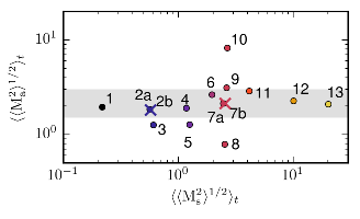
Figure 1: Parameter space covered by the 15 simulations. Each marker (circles for a resolution of $512^{3}$ grid-points and crosses for $1024^{3}$, respectively) corresponds to the respective mean value over the stationary phase $2T<t<5T$ of the spatial root mean square Mach numbers. Only simulations within the gray area are used in the detailed sonic Mach number dependency study. Simulation details are given in table 1.

Simulations 1, 2a, 4, 6, 7a, 11, 12, 13 within the gray area have $\langle\langle\mathrm{M}_{\mathrm{a}}^{2}\rangle^{1/2}\rangle_{t}\approx 3$ and are therefore used for a $\mathrm{M_{s}}$-dependency analysis of the different closures.

III.2 Reference quantities

In order to assess the quality and performance of the different closures we conduct functional and structural a priori tests. In a priori testing a test filter is applied to high resolution data to mimic the effect of limited resolution. The scales below the test filter are treated as unresolved scales. Owing to the explicit filtering we not only obtain filtered quantities intended to resemble the resolved scales, but also retain the sub-filter quantities intended to resemble the unresolved scales. This allows the exact calculation of SGS quantities. In the context of LES three different filter kernels are typically usedSagaut (2006): the box, the Gaussian, and the sharp spectral filter. For the majority of our analysis we use a Gaussian filter with a characteristic filter scale at a wavenumber $k=16$ for several reasons. Firstly, $k=16$ is within a power-law regime of the energy spectra (cf. figure 2), which satisfies the assumption of the eddy-viscosity and scale-similarity type closures. Secondly, it is sufficiently far away from the forcing scale $k=2$ where the dynamics of the forcing are expected to be dominant. Thirdly, it also does not fall above the high-$k$ drop-off in the spectrum, caused by viscous and numeric dissipation, which contaminates turbulent dynamics Kitsionas et al. (2009). The mean spectra within the stationary regime ($2T<t<5T$) of the simulations are illustrated in figure 2, where we also highlight the filter positions.

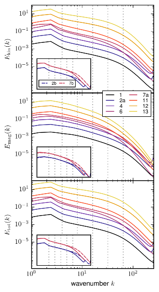
Figure 2: Mean ($2T<t<5T$) power spectra of the simulations. Kinetic energy is based on the Fourier transform of $\sqrt{\rho}\bm{u}$. The dashed vertical lines indicate the filter widths ($k=4,8,16,32,64$) we are using during the analysis. The insets highlight the extended power-law regime of the $1024^{3}$ runs (2b and 7b, dashed lines) over the corresponding $512^{3}$ runs (2a and 7a, solid lines). Simulation details are listed in table 1.

In addition to filtering at $k=16$ we also probe the closures with filter scales at $k=4,8,32,64$ to investigate the dependence of the result on the chosen scale. Moreover, we verify the results based on Gaussian filtering against a box filter. Given that we analyze compressible data, we do not employ a sharp spectral filter, which can produce negative resolved densities, and SGS stresses that violate realizabilityVreman, Geurts, and Kuerten (1994).

The first category of tests, functional tests, probe the ability of closures to reproduce a particular (physical) property. In addition to this, functional tests can eliminate co-ordiate frame dependence by reduction to scalar diagnostics, e.g. of six SGS stress tensor or three EMF vector components. Historically, the most frequently used reference quantity is the turbulent energy flux, i.e. the cascade term

$$\Sigma^{E}=\tau_{ij}\widetilde{\mathcal{S}}_{ij}+{\bm{\mathcal{E}}}\cdot\overline{\bm{J}}\;.$$ (79)

It encodes the local exchange between resolved and unresolved energy and is connected to the turbulent energy cascade. However, as it was recently shownVlaykov (2015), the total energy flux term

$$\mathcal{F}^{E}=-\widetilde{\bm{u}}\cdot\left(\nabla\cdot\tau\right)+\overline{\bm{B}}\cdot\nabla\times{\bm{\mathcal{E}}}$$ (80)

is more strongly influenced by the transport terms ${\nabla\cdot\left(\widetilde{\bm{u}}\cdot\tau+\overline{\bm{B}}\times{\bm{\mathcal{E}}}\right)}$ rather than the cascade term $\Sigma^{E}$ in our simulations. Furthermore, in MHD there are additional conserved quantities such as cross-helicity, ${W=\bm{u}\cdot\bm{B}}$, which are, in the context of LES, also governed by resolved and subgrid-scale evolution equationsVlaykov (2015). The exchange of cross-helicity across the filter scale is analogous to the energy one, with cross-helicity flux

$$\Sigma^{W}=\tau_{ij}\left(\overline{B_{i}}/\overline{\rho}\right)_{,j}+{\bm{\mathcal{E}}}\cdot\widetilde{\bm{\Omega}}\;.$$ (81)

Again, the total cross-helicity term

$$\mathcal{F}^{W}=-\overline{\bm{B}}/\overline{\rho}\cdot\left(\nabla\cdot\tau\right)+\widetilde{\bm{u}}\cdot\nabla\times{\bm{\mathcal{E}}}\;,$$ (82)

is dominated by the transport and not the cascade contributionVlaykov (2015). In the following we are going to analyze all four (pseudo-)scalars as each of them may play a crucial role in different dynamical regimes, and systematic differences between results from total and cascade fluxes may indicate the importance of the differentiation commutatorVlaykov et al. (2016). Specifically, we conduct nonlinear least-square minimizationNewville et al. (2014) between data and closure. This automatically produces the best coefficient $C_{\Box}$ for each snapshot and closure individually. Eventually, we calculate the Pearson correlation coefficient as an overall measure of accuracy. While these correlations probe the spatially local performance of the closures, we also analyze a global indicator. In particular, we look at the average SGS dissipation, i.e. the total $\Sigma^{E}$ for each snapshot, and examine the contributions of the individual components.

The performed structural tests start with a topological analysis. We use the geometric invariants of second-rank tensors to compare the topology of the deviatoric SGS Reynolds $\tau^{\mathrm{u}*}$ and Maxwell $\tau^{\mathrm{b}*}$ stress tensors for data and closure. The characteristic polynomial of a second-rank tensor $\mathcal{T}$ isDallas and Alexakis (2013) $\lambda_{i}^{3}+P\lambda_{i}^{2}+Q\lambda_{i}+R=0$ with eigenvalues $\lambda_{i}$ and invariants

$$P = -\operatorname{tr}\left(\mathcal{T}\right)=-\left(\lambda_{1}+\lambda_{2}+\lambda_{3}\right)\;,$$ (83)

$$Q = \frac{1}{2}\left(P^{2}-\operatorname{tr}{\left(\mathcal{T}^{2}\right)}\right)=\lambda_{1}\lambda_{2}+\lambda_{2}\lambda_{3}+\lambda_{3}\lambda_{1}\;,$$ (84)

$$R = -\det\left(\mathcal{T}\right)=-\lambda_{1}\lambda_{2}\lambda_{3}\;.$$ (85)

Both tensors, $\tau^{\mathrm{u}*}$ and $\tau^{\mathrm{b}*}$, are traceless, so $P=0$. Furthermore, they are symmetric. Thus, $Q$ is negative definite and the three eigenvalues $\lambda_{1}\geq\lambda_{2}\geq\lambda_{3}$ are real. Therefore, only two eigenvalue combinations are possible. On the one hand, sheet-like structures with $R>0$ are produced by expansion in two dimensions ($\lambda_{1},\lambda_{2}>0$), and contraction in the third dimension ($\lambda_{3}<0$). On the other hand, tube-like structures with $R<0$ are produced by expansion in one dimension ($\lambda_{1}>0$), and contraction in two dimensions ($\lambda_{2},\lambda_{3}<0$).

Given that all closures enter the primary equations ultimately in vectorial form, we also asses their geometrical performance. For this reason, we compare the alignment of the data vector, e.g. $\nabla\cdot\tau^{\mathrm{u}*}$, with the corresponding closure vector, i.e. $\nabla\cdot\widehat{\tau}_{ij}^{\mathrm{u}*}$. Moreover, we compare their respective magnitudes. Ideally, the modeled SGS vector will point in the identical direction as the data vector ($\cos\left(\nabla\cdot\widehat{\tau}_{ij}^{\mathrm{u}*},\nabla\cdot\tau^{\mathrm{u}*}\right)=1$), and will be with identical magnitude ($|\nabla\cdot\widehat{\tau}_{ij}^{\mathrm{u}*}|/|\nabla\cdot\tau^{\mathrm{u}*}|=1$).

IV Results

IV.1 Functional analysis: overview and $\mathrm{M_{s}}$ dependency

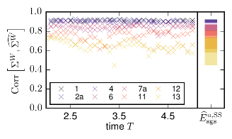
Figure 3: Illustration of using correlations from individual simulation snapshots (left) to create a bar plot (right). Each marker on the left side corresponds to the correlation coefficient from one snapshot of the color-coded simulations from the subsonic (dark) to the hypersonic (bright) regime. The correlation coefficient is always calculated for only one reference quantity (here, the cross-helicity cascade flux $\Sigma^{W}$) with one closure (here, the kinetic SGS energy of the scale-similarity family $\widehat{E}^{\mathrm{u},\mathrm{SS}}_{\mathrm{sgs}}$). Each colored bar on the right side spans the range of variation from the minimum to the maximum correlation value over all snapshots of one simulation.

We start our functional analysis by evaluating the performance of the different closures for the isotropic parts of the SGS stresses, i.e. by definition (8), the SGS energies $\tau_{ij}^{\Box}=2/3\delta_{ij}E_{\mathrm{sgs}}^{\Box}$. Figure 3 illustrates the creation of the Mach number dependent bar plots we use in this section for one sample quantity. We use the kinetic SGS energy closure of the scale-similarity family $\widehat{E}^{\mathrm{u},\mathrm{SS}}_{\mathrm{sgs}}$ (61), and compute the correlation $\mathrm{Corr}\left[\Sigma^{W},\widehat{\Sigma^{W}}\right]$ of the contribution to cross-helicity cascade term $\Sigma^{W}$ based on closure and exact SGS energy expression $E^{\mathrm{u}}_{\mathrm{sgs}}$ (7), i.e.

$$\mathrm{Corr}\left[\frac{2}{3}\delta_{ij}E^{\mathrm{u}}_{\mathrm{sgs}}\left(\frac{\overline{B_{i}}}{\overline{\rho}}\right)_{,j},\frac{2}{3}\delta_{ij}\widehat{E}^{\mathrm{u},\mathrm{SS}}_{\mathrm{sgs}}\left(\frac{\overline{B_{i}}}{\overline{\rho}}\right)_{,j}\right]\;.$$ (86)

This is done for each snapshot of all simulations. Then, we take the minimum and maximum value of each simulation separately to determine the vertical extent of the color-coded bars in the right panel of the figure. In this example it is clear that the cross-helicity cascade is well modeled in the subsonic regime (with correlations above 0.8) and tends to perform worse in the hypersonic regime (going down to almost 0.4).

The results for all energy closures and all reference quantities are shown in figure 4(a). In general, all closures perform very well with respect to the cascade fluxes. A notable exception is the already mentioned cross-helicity cascade correlation of the kinetic scale-similarity model $\widehat{E}^{\mathrm{u},\mathrm{SS}}_{\mathrm{sgs}}$, which has a strong $\mathrm{M_{s}}$ dependency. In addition to this, it can be seen that the total flux terms are generally less well represented than the cascade terms. Furthermore, there is practically no difference between modeling the eddy-viscosity/diffusivity energies based on realizability conditions ($\widehat{E}^{\mathrm{u},\mathcal{S}^{*}}_{\mathrm{sgs}}$ and $\widehat{E}^{\mathrm{b},\mathcal{M}}_{\mathrm{sgs}}$) and the equilibrium approach ($\widehat{E}^{\mathrm{u},\mathcal{S}}_{\mathrm{sgs}}$ and $\widehat{E}^{\mathrm{b},J}_{\mathrm{sgs}}$). Overall, with a slight advantage over the eddy-viscosity closures, the nonlinear closures perform best with generally high correlations (>$0.7$ across the entire parameter space) and very limited $\mathrm{M_{s}}$ dependency. The median across all simulations of the free coefficient value of each closure is listed in table 2 including bounds given by the interquartile range (IQR). For reference we also provide more detailed data tables as supplemental materialsup . All SGS energy closures exhibit only a very limited spread over the tested parameter space with IQRs within a factor of 2 around the median. These results also hold (not shown) for direct fits, i.e. $\mathrm{Corr}\left[E_{\mathrm{sgs}}^{\Box},\widehat{E}_{\mathrm{sgs}}^{\Box}\right]$, of the kinetic $E^{\mathrm{u}}_{\mathrm{sgs}}$, magnetic $E^{\mathrm{b}}_{\mathrm{sgs}}$, and total $E_{\mathrm{sgs}}$ energies.

Table 2: Median correlation and coefficient values over all $512^{3}$ simulations filtered at $k=16$ with lower and upper bound given by interquartile range of all data. Detailed data tables including results split by reference quantity and min-/maximum values can be found in the supplementary materialsup .

ID	$\mathrm{Corr}\left[\Box,\widehat{\Box}\right]$	Coefficient
$\widehat{E}^{\mathrm{u},\mathcal{S}}_{\mathrm{sgs}}$	$0.83^{+0.082}_{-0.094}$	$C_{4}=0.036^{+0.014}_{-0.0074}$
$\widehat{E}^{\mathrm{u},\mathcal{S}^{*}}_{\mathrm{sgs}}$	$0.84^{+0.068}_{-0.098}$	$C_{2}=0.038^{+0.022}_{-0.005}$
$\widehat{E}^{\mathrm{u},\mathrm{SS}}_{\mathrm{sgs}}$	$0.59^{+0.3}_{-0.11}$	$C_{21}=1^{+0.19}_{-0.35}$
$\widehat{E}^{\mathrm{u},\mathrm{NL}}_{\mathrm{sgs}}$	$0.85^{+0.077}_{-0.058}$	$C_{24}=1.2^{+0.53}_{-0.19}$
$\widehat{E}^{\mathrm{b},J}_{\mathrm{sgs}}$	$0.83^{+0.057}_{-0.084}$	$C_{3}=0.043^{+0.021}_{-0.0065}$
$\widehat{E}^{\mathrm{b},\mathcal{M}}_{\mathrm{sgs}}$	$0.87^{+0.054}_{-0.13}$	$C_{1}=0.045^{+0.028}_{-0.0058}$
$\widehat{E}^{\mathrm{b},\mathrm{SS}}_{\mathrm{sgs}}$	$0.79^{+0.093}_{-0.23}$	$C_{22}=1.1^{+0.26}_{-0.36}$
$\widehat{E}^{\mathrm{b},\mathrm{NL}}_{\mathrm{sgs}}$	$0.93^{+0.018}_{-0.073}$	$C_{25}=1.3^{+0.43}_{-0.1}$
$\mathrm{EV}^{\mathrm{const}}$	$0.4^{+0.079}_{-0.12}$	$C_{5}=0.096^{+0.13}_{-0.074}$
$\mathrm{EV}^{\mathcal{SM}}$	$0.35^{+0.081}_{-0.1}$	$C_{8}=0.011^{+0.0061}_{-0.0057}$
$\mathrm{EV}^{W}$	$0.39^{+0.092}_{-0.12}$	$C_{10}=0.024^{+0.008}_{-0.008}$
$\mathrm{EV}^{\mathcal{S^{*}}}$	$0.43^{+0.091}_{-0.13}$	$C_{16}=0.0085^{+0.0031}_{-0.0031}$
$\mathrm{EV}^{E}$	$0.44^{+0.089}_{-0.15}$	$C_{13}=0.041^{+0.017}_{-0.021}$
$\mathrm{ED}^{\mathrm{const}}$	$0.02^{+0.016}_{-0.012}$	$C_{6}=0.00071^{+-0.006}_{-0.006}$
$\mathrm{ED}^{W}$	$0.089^{+0.1}_{-0.042}$	$C_{11}=-0.0066^{+0.0025}_{-0.0067}$
$\mathrm{ED}^{\mathcal{M}}$	$0.026^{+0.021}_{-0.012}$	$C_{17}=0.00014^{+0.00014}_{-0.00038}$
$\mathrm{ED}^{E}$	$0.027^{+0.02}_{-0.014}$	$C_{14}=0.00055^{+0.00093}_{-0.002}$
$\mathrm{ER}^{\mathrm{const}}$	$0.35^{+0.092}_{-0.053}$	$C_{7}=0.14^{+0.054}_{-0.11}$
$\mathrm{ER}^{\mathcal{SM}}$	$0.032^{+0.024}_{-0.017}$	$C_{9}=-0.00055^{+0.0011}_{-0.0015}$
$\mathrm{ER}^{W}$	$0.042^{+0.035}_{-0.024}$	$C_{12}=-0.0014^{+0.0021}_{-0.0039}$
$\mathrm{ER}^{\mathcal{S+M}}$	$0.36^{+0.11}_{-0.057}$	$C_{18}=0.0096^{+0.0068}_{-0.0035}$
$\mathrm{ER}^{E}$	$0.36^{+0.1}_{-0.056}$	$C_{15}=0.035^{+0.025}_{-0.013}$
$\alpha\text{-}\beta\text{-}\gamma$	$0.37^{+0.11}_{-0.049}$	$\left\{\begin{tabular}[]{@{\ }l@{}}$C_{20}=-0.0026^{+0.0018}_{-0.0043}$\\ $C_{15}=0.033^{+0.028}_{-0.0087}$\\ $C_{19}=-0.00017^{+0.0058}_{-0.0079}$\\ \end{tabular}\right.$
$\mathrm{SS}^{\mathrm{u}}$	$0.49^{+0.11}_{-0.072}$	$C_{21}=0.67^{+0.16}_{-0.23}$
$\mathrm{SS}^{\mathrm{b}}$	$0.58^{+0.081}_{-0.084}$	$C_{22}=0.9^{+0.25}_{-0.43}$
$\mathrm{SS}^{\mathcal{E}}$	$0.55^{+0.13}_{-0.084}$	$C_{23}=0.89^{+0.098}_{-0.18}$
$\mathrm{NL^{u}}$	$0.82^{+0.038}_{-0.029}$	$C_{24}=0.98^{+0.081}_{-0.19}$
$\mathrm{NL}^{\mathrm{u,\mathcal{S^{*}}}}$	$0.77^{+0.069}_{-0.038}$	$C_{30}=0.032^{+0.0026}_{-0.0052}$
$\mathrm{NL}^{\mathrm{u,E}}$	$0.81^{+0.078}_{-0.13}$	$C_{28}=0.52^{+0.09}_{-0.12}$
$\mathrm{NL^{b}}$	$0.85^{+0.029}_{-0.038}$	$C_{25}=1.1^{+0.19}_{-0.063}$
$\mathrm{NL}^{\mathrm{b,\mathcal{M}}}$	$0.77^{+0.065}_{-0.074}$	$C_{31}=0.039^{+0.0093}_{-0.0052}$
$\mathrm{NL}^{\mathrm{b,E}}$	$0.76^{+0.11}_{-0.14}$	$C_{29}=0.52^{+0.21}_{-0.21}$
$\mathrm{NL}^{\mathcal{E}}$	$0.7^{+0.13}_{-0.13}$	$C_{27}=1.2^{+0.14}_{-0.11}$
$\mathrm{NL}^{\mathcal{E},\rho}$	$0.84^{+0.04}_{-0.072}$	$C_{26}=1^{+0.11}_{-0.3}$

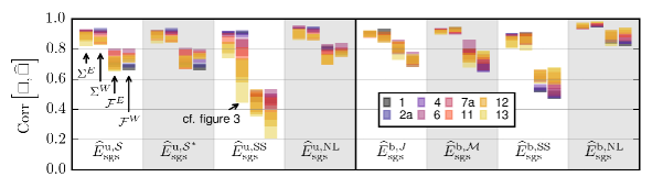
(a) Correlations of different SGS energy closures, i.e. the isotropic component of the SGS stress tensors.

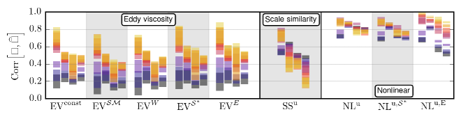
(b) Correlations of different traceless SGS Reynolds stress $\tau^{\mathrm{u}*}$ closures.

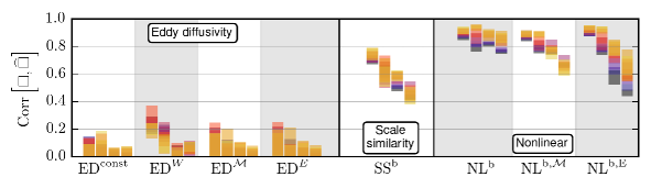
(c) Correlations of different traceless SGS Maxwell stress $\tau^{\mathrm{b}*}$ closures.

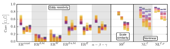
(d) Correlations of different electromotive force $\mathcal{E}$ closures.

Figure 4: Correlations between closure and data for all reference fluxes. For each closure the four colored bars (from left to right: energy $\Sigma^{E}$ and cross-helicity $\Sigma^{W}$ cascade, and total energy $\mathcal{F}^{E}$ and cross-helicity $\mathcal{F}^{W}$ flux) illustrate the maximum range of correlation split by simulation. A detailed explanation of the colored bars is given in figure 3. Subsonic runs are towards the dark end and supersonic at the bright end of the palette (cf. figure 2). All simulations have been filtered at $k=16$. The x-axis labels denote the different closure identifiers as introduced in section II.

The correlations of all four functional reference quantities for the traceless SGS Reynolds stress $\widehat{\tau}_{ij}^{\mathrm{u}*}$ are depicted in figure 4(b). All eddy-viscosity type closures $\mathrm{EV}^{\Box}$ are very similar and insensitive of the scaling chosen. Even though the correlations for all snapshots within a single simulation do not vary much, there is a substantial difference between the simulations. Correlations are typically below $0.2$ in the subsonic regime whereas they can reach >$0.8$ in the highly supersonic regime. This ordering is present in all reference quantities for the $\mathrm{EV}$ closures. The scale-similarity $\mathrm{SS}^{\mathrm{u}}$ closure also exhibits this behavior for the turbulent energy cascade $\Sigma^{E}$ even though the lower bound in the subsonic regime is much better, $\approx 0.5$. However, the correlations of the other fluxes, $\Sigma^{W}$, $\mathcal{F}^{E}$ and $\mathcal{F}^{W}$, have the opposite ordering. The most extreme case of $\mathcal{F}^{W}$ spreads from $\approx 0.5$ in the subsonic regime to correlations as low as $0.1$ for the $\mathrm{M_{s}}\approx 20$ simulation. The nonlinear family $\mathrm{NL}$ is closest to the data in general. Again, we observe an ordering with $\mathrm{M_{s}}$ but the spread is much more constrained and for $\mathrm{NL^{u}}$ the correlations are consistently above $0.7$. Here, the scaling only further separates individual simulations with supersonic simulations slightly improving and subsonic simulations becoming worse on average.

Generally, the results for the traceless SGS Maxwell stress $\widehat{\tau}_{ij}^{\mathrm{b}*}$, as shown in figure 4(c), are very similar to those for $\widehat{\tau}_{ij}^{\mathrm{u}*}$. Again, the nonlinear family has the best performance and different normalizations for $\mathrm{NL}$ cause a wider spread. The scale-similarity closure $\mathrm{SS}^{\mathrm{b}}$ is slightly worse with best correlations up to $0.8$ for $\Sigma^{E}$ and worst – $0.4$ for $\mathcal{F}^{W}$. Most striking is the poor performance of all eddy-diffusivity ($\mathrm{ED}$) closures. Independent of normalization and simulation the correlations barely reach $0.4$ with the majority of snapshots (93%) being below $0.2$ for all reference quantities.

Finally, the findings for the electromotive force ${\bm{\mathcal{E}}}$ are much more diverse. Firstly, within the eddy-resistivity ($\mathrm{ER}$) family, scaling by cross-helicity leads to poor correlations (99% snapshots below $0.2$). However, $\mathrm{ER}^{\mathrm{const}}$ and energy scalings ($\mathrm{ER}^{\mathcal{SM}}$ and $\mathrm{ER}^{E}$) provide reasonable correlations (from $0.5$ for low $\mathrm{M_{s}}$ to $0.7$ for high $\mathrm{M_{s}}$) for the turbulent energy cascade $\Sigma^{E}$, but are less effective (<$0.5$) for $\Sigma^{W}$, $\mathcal{F}^{E}$ and $\mathcal{F}^{W}$. In addition, there is practically no difference between these scalings and the addition of the two extra terms in the $\alpha\text{-}\beta\text{-}\gamma$ closure. Secondly, the scale-similarity closure $\mathrm{SS}^{\mathcal{E}}$ performs similar to the reasonable $\mathrm{ER}$ closures with respect to the total terms $\mathcal{F}^{E}$ and $\mathcal{F}^{W}$. However, it performs much better for the cascade terms with correlations for $\Sigma^{W}$ of $\approx 0.65$ and for $\Sigma^{E}$ of $\approx 0.75$ without significant $\mathrm{M_{s}}$ dependence. Thirdly, the effect of the compressible extension of the nonlinear closure $\mathrm{NL}^{\mathcal{E},\rho}$ becomes apparent when comparing the results for different simulations. While there is practically no difference between $\mathrm{NL}^{\mathcal{E}}$ and $\mathrm{NL}^{\mathcal{E},\rho}$ in the subsonic regime (correlations >$0.9$ for all quantities), the shortcomings of $\mathrm{NL}^{\mathcal{E}}$ in the highly supersonic regime are apparent. Correlations of $\approx 0.4$ for $\Sigma^{W}$, $\mathcal{F}^{E}$ and $\mathcal{F}^{W}$ in the $\mathrm{M_{s}}\approx 20$ simulation can be improved by the additional term in $\mathrm{NL}^{\mathcal{E},\rho}$ to $\approx 0.6$ for $\mathcal{F}^{E}$ and $\mathcal{F}^{W}$, and even up to $\approx 0.8$ for $\Sigma^{W}$. The improvements for $\mathrm{NL}^{\mathcal{E},\rho}$ are more pronounced in the cascade terms (with a spread of 0.8-0.9) than in the total flux terms (with a spread of 0.6-0.9). Here, the additional differentiation commutatorVlaykov et al. (2016) might further increase the correlations in the high-$\mathrm{M_{s}}$ regime. The overall trend that the nonlinear closures are better correlated with the data than the scale-similarity or eddy-resistivity closures continues for the electromotive force as well.

Furthermore, as listed in table 2 closures that exhibit a generally high correlation show the least spread in their free coefficient values $C_{\Box}$ and vice versa. For example, $\mathrm{NL^{u}}$, with a median correlation of $0.82$, has a spread in the coefficient value of <$20\%$. In contrast to this, $\mathrm{ED}^{E}$, with a median correlation of $0.027$, has median coefficient of effectively $0$ because it takes both negative and positive values. It should be noted that all scale-similarity closures and the unnormalized nonlinear closures have coefficients of $C_{\Box}\approx 1$, as expected analytically. Finally, the common coefficient $C_{15}$, which the $\alpha\text{-}\beta\text{-}\gamma$ and $\mathrm{ER}^{E}$ closures share, is essentially identical, while the two additional terms in the $\alpha\text{-}\beta\text{-}\gamma$ closure are effectively canceled by their free coefficients $C_{19},C_{20}\approx 0$. This also explains their identical behavior in correlations.

IV.2 Functional analysis: filter widths and kernel shapes

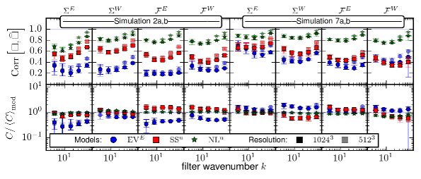
(a) SGS Reynolds stress closures $\widehat{\tau}_{ij}^{\mathrm{u}*}$

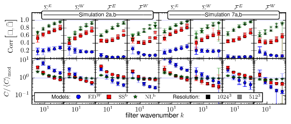
(b) SGS Maxwell stress closures $\widehat{\tau}_{ij}^{\mathrm{b}*}$

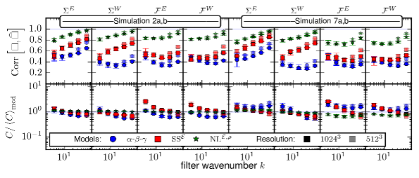
(c) Electromotive force closures $\widehat{\bm{\mathcal{E}}}$

Figure 5: Comparison of the median correlation (top row in each plot) and coefficient (bottom row) value at different filter wavenumbers $k=4,8,16,32,64$ and simulation resolutions $512^{3}$ (transparent) and $1024^{3}$ (opaque) for subsonic simulation 2a,b and supersonic simulation 7a,b. The error bars illustrate the respective minimum and maximum values. Each column corresponds to results of fitting one reference quantity $\Sigma^{E}$, $\Sigma^{W}$, $\mathcal{F}^{E}$ or $\mathcal{F}^{W}$, and each marker represents the median value over snapshots at $t=\{2,2.5,3,3.5,4,4.5,5\}T$ of the particular simulation. The coefficient values are normalized to the respective median value over the snapshots of both simulations and at all filter widths at a given resolution.

In the last section we saw that the differences in correlations for functional tests are most pronounced between closure families and that normalization within a family itself is subdominant. For this reason, we continue our analysis with the best performing closure of each family. In this section we verify that the results shown in the last section from simulations at a resolution of $512^{3}$ filtered at $k=16$ do not substantially change with resolution and we investigate how the different closures react to the chosen filter scale.

Figure 5 illustrates the comparison of correlation and coefficient values among four simulations (2a,b and 7a,b) that differ in driving (subsonic and supersonic) and resolution ($512^{3}$ and $1024^{3}$). Furthermore, we apply the filter at different scales $k=4,8,16,32,64$. The extreme cases, $k=4$ and $k=64$, are very close to the forcing regime or already in the dissipation regimeKitsionas et al. (2009), respectively. Generally, we confirm the observed ordering in correlations among closure families described in the last section. Independent of resolution and filter width, the nonlinear closures outperform the scale-similarity and eddy-viscosity type closures. On average the difference in both correlations and coefficient values between the $512^{3}$ and $1024^{3}$ simulations are below 7% at $k=16$. Furthermore, all closures typically achieve higher correlations ($\approx 25\%$ while filtering at $k=64$ compared to $k=16$) towards the high-$k$ end and the correlations from $512^{3}$ simulations at $k>16$ tend to be higher than from simulations at $1024^{3}$. This is not surprising. On the one hand, the amount of subgrid-scale dynamics that needs to be modeled is reduced with increasing filter wavenumber. One the other hand, there is less physical information at high $k$ for lower resolutions. Nevertheless, for some cases there are more subtle differences with respect to filter scale, which we describe in the following.

In figure 5(a) the best closures within each family for the SGS Reynolds stress are shown, i.e. $\mathrm{EV}^{E}$, $\mathrm{SS}^{\mathrm{u}}$ and $\mathrm{NL^{u}}$. The overall correlation, depending on filter scale $k$, for each model and reference quantity has a very shallow U-shape. Compared to $k=16$, the correlations are $\approx 6\%$ higher at $k=4$ and $\approx 30\%$ higher at $k=64$, respectively. The slight increase at $k=4$ might be attributed to the proximity to the forcing scale $k\approx 2$, which is completely resolved. Thus, the largest unresolved scales of $\tau^{\mathrm{u}}$ might see an imprint of the (resolved) forcing and lack SGS turbulent dynamics, which, in turn, renders specific SGS modeling unnecessary and increases the correlation. The observed systematic differences in correlations with varying $k$ are generally not present in the coefficient values. However, the values vary to different extents within each family and reference quantity. While the mean deviation from the median coefficient over all reference quantities, filter widths and snapshots is only 10% for the nonlinear closure $\mathrm{NL^{u}}$, it varies by $47\%$ for the eddy-viscosity reference closure $\mathrm{EV}^{E}$. Compared to the results of $\tau^{\mathrm{b}*}$ in the next paragraph, this is still acceptable, even though we find systematically lower coefficient at $\mathrm{M_{s}}\approx 0.6$ compared to $\mathrm{M_{s}}\approx 2.5$.

The SGS Maxwell stress results depicted in figure 5(b) show a strong filter scale dependency of the closure coefficient for the scale-similarity $\mathrm{SS}^{\mathrm{b}}$ and eddy-diffusivity $\mathrm{ED}^{W}$ closure. The coefficients are larger for small $k$ and decrease with increasing $k$ spanning almost two orders-of-magnitude. Only the nonlinear closure $\mathrm{NL^{b}}$ keeps a rather constant value with deviations of $17\%$ on average. The correlations, on the other hand, show a systematic increase with $k$ for $\mathrm{NL^{b}}$ in all reference quantities. This might be ascribed to the absence of a direct forcing term acting on the magnetic field. Similar behavior is also present in $\mathrm{SS}^{\mathrm{b}}$ with the slight difference of a plateau for $k\leq 16$ in the total flux quantities $\mathcal{F}^{E}$ and $\mathcal{F}^{W}$. Finally, the eddy-diffusivity closure never reaches a correlation higher than $0.36$ over the entire parameter space.

The different closures for the electromotive force ${\bm{\mathcal{E}}}$ are closer to each other as illustrated in figure 5(c). Here, both $\mathrm{NL}^{\mathcal{E},\rho}$ and $\mathrm{SS}^{\mathcal{E}}$ exhibit strictly increasing correlation values with $k$ for the cascade terms $\Sigma^{E}$ and $\Sigma^{W}$ and a plateau for $k\leq 16$ in the total flux terms $\mathcal{F}^{E}$ and $\mathcal{F}^{W}$. The coefficient values for all ${\bm{\mathcal{E}}}$ closure are less widely spread. The $\alpha\text{-}\beta\text{-}\gamma$ closure has a variation of $37\%$ around the median over all data whereby we only take the dominant $\beta$ term into account. The $\mathrm{SS}^{\mathcal{E}}$ closure has a variation of $47\%$ and the nonlinear closure is effectively constant with a spread of only $16\%$.

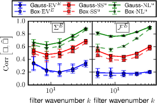
Figure 6: Correlations of the energy cascade, $\Sigma^{E}$, and total energy, $\mathcal{F}^{E}$, flux of different deviatoric kinetic SGS stress closures for different filter widths and kernels (box - - and Gaussian —) in subsonic simulation 2b. Markers indicate the median and the error bars show the minimum and maximum value over time.

Finally, the differences between using a Gaussian and a box kernel for the analysis are illustrated in figure 6. Two trends can be observed for the kinetic energy cascade and total flux. The correlations of $\Sigma^{E}$ for the box filter are (within the error bars) slightly lower ($\lesssim 10\%$) for all models and filter widths. In addition, the correlations exhibit a more pronounced deviation for the total energy flux $\mathcal{F}^{E}$ especially at smaller filter wavenumbers $k$ and thus larger filter widths. We attribute this to the non-smooth nature of the box kernel versus the Gaussian kernel resulting in numerical biases in the computation of gradient-based quantities. This could explain why the deviations are more pronounced in the total flux that has an additional divergence operator acting on the SGS terms in comparison to the cascade flux. Likewise, the effect would be more pronounced in the nonlinear closures as they are built from nonlinear combinations of gradients. The observed convergence between box and Gaussian filtering with increasing $k$ is also expected, because the differences between the kernels become less distinct for small widths. Overall, the observed behavior based on Gaussian filtering, i.e. better performance of the nonlinear closures over the scale-similarity and the eddy-dissipation family ones, also holds for filtering with a box kernel. These trends similarly apply to the cross-helicity fluxes and other SGS terms, too.

IV.3 Functional analysis: average SGS dissipation

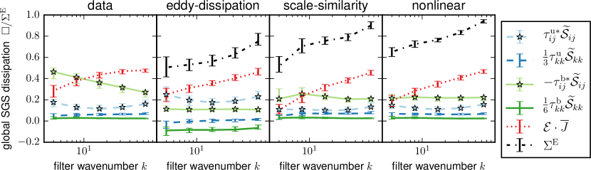
Figure 7: Contributions of individual components (deviatoric kinetic SGS stress, $\tau_{ij}^{\mathrm{u}*}\widetilde{\mathcal{S}}_{ij}$, and deviatoric magnetic SGS stress, $\tau_{ij}^{\mathrm{b}*}\widetilde{\mathcal{S}}_{ij}$, kinetic SGS pressure, $1/3\tau^{\mathrm{u}}_{kk}\widetilde{\mathcal{S}}_{kk}$, and magnetic SGS pressure, $1/6\tau^{\mathrm{b}}_{kk}\widetilde{\mathcal{S}}_{kk}$, and EMF, ${\bm{\mathcal{E}}}\cdot\overline{\mathbf{J}}$) normalized to the average SGS dissipation, $\Sigma^{E}$, of supersonic simulation 7b for different filter widths. The markers illustrate the median and the error bars show the minimum and maximum values over time. Each closure family is represented by the locally best performing closures, i.e. eddy-dissipation of $\mathrm{EV}^{E}$-$\widehat{E}^{\mathrm{u},\mathcal{S}}_{\mathrm{sgs}}$-$\mathrm{ED}^{W}$-$\widehat{E}^{\mathrm{b},J}_{\mathrm{sgs}}$-$\alpha\text{-}\beta\text{-}\gamma$, scale-similarity of $\mathrm{SS}^{\mathrm{u}}$-$\mathrm{SS}^{\mathrm{b}}$-$\mathrm{SS}^{\mathcal{E}}$, and the nonlinear family of $\mathrm{NL^{u}}$-$\mathrm{NL^{b}}$-$\mathrm{NL}^{\mathcal{E},\rho}$.

We close the functional analysis with a comparison of the contributions by individual components to the average SGS dissipation $\Sigma^{E}$. Figure 7 illustrates the share of deviatoric kinetic SGS stress, $\tau_{ij}^{\mathrm{u}*}\widetilde{\mathcal{S}}_{ij}$, and deviatoric magnetic SGS stress, $\tau_{ij}^{\mathrm{b}*}\widetilde{\mathcal{S}}_{ij}$, kinetic SGS pressure, $1/3\tau^{\mathrm{u}}_{kk}\widetilde{\mathcal{S}}_{kk}$, and magnetic SGS pressure, $1/6\tau^{\mathrm{b}}_{kk}\widetilde{\mathcal{S}}_{kk}$, and EMF, ${\bm{\mathcal{E}}}\cdot\overline{\mathbf{J}}$ to $\Sigma^{E}$ for different filter widths. In general, both SGS pressures (and thus energies) are almost negligible ($<10\%$) in the reference data even though the data covers the slightly supersonic regime (simulation 7b). Similarly, the deviatoric kinetic SGS stress is subdominant ($10\%$-$20\%$) while the deviatoric magnetic SGS stress and the EMF, which jointly contribute $\approx 80\%$ to the total SGS dissipation independent of the chosen filter scale. While the magnetic stress dominates at the largest scales (up to $50\%$ at $k=4$), its contribution constantly decreases, and at the smallest scale the EMF is strongest reaching a contribution of $\approx 50\%$. This can be understood by analyzing the ratio of forward to inverse energy transfer (not shown). While the forward transfer mediated by $\tau_{ij}^{\mathrm{b}*}\widetilde{\mathcal{S}}_{ij}$ is $\approx 30$ times stronger than the inverse transfer at $k=4$, it is only $\approx 6$ times stronger at $k=64$. At the same time the ratio by the EMF remains constantly at a factor $\approx 8$. Two scenarios (or more likely an unbalanced combination thereof) could potentialy explain this situation: either the existance of an inverse cascade coupled to direct forward transfer, or direct inverse transfer coupled with a forward cascade. On the one hand, a cascade typically transfers energy from one scale to the next smaller (or larger) scale resulting in a constant flux with varying filter width. On the other hand, direct transfer allows exchange of energy between scales with arbitrary separation and thus the flux may vary with varying filter width. Although a more detailed study, e.g. by a shell-to-shell energy transfer analysis, would allow a better interpretation, it is not required for the following closure discussion and we leave it as subject to future work.

Before analyzing the predicted contributions by the different closure families, it should be noted that the coefficient from the fit has been used to calculate the resulting dissipation values. Allowing all coefficients to vary freely and optimizing for average SGS dissipation would allow each closure to excatly match the reference data and, in turn, render this analysis meaningless. In general, all closure families behave similar with respect to the total dissipation. At large scales they underestimate the reference data by $\approx 50\%$ (eddy-dissipation and scale-similarity) and $\approx 40\%$ (nonlinear), while improving towards the smallest scales reaching $\approx 75\%$ ($\mathrm{ED}$), $\approx 90\%$ ($\mathrm{SS}$) and $\approx 95\%$ ($\mathrm{NL}$) agreement. This is seen to be due to the successful capture of the EMF related contribution and failing to represent the deviatoric magnetic stress dynamics at varying filter scale. In other words, all closures predict too much net inverse energy transfer to the largest scales. Another important observation concerns the overall inverse energy transfer by the magnetic SGS pressure of the eddy-diffusivity closure. Given that the eddy-viscosity and eddy-resistivity closures can not provide inverse energy transfer by construction, and that the eddy-diffusivity closure itself exhibits the overall poorest correlation as shown in the previous subsections, the SGS pressures are the only channels left for inverse transfer in this closure set. Thus, in the process of matching the inverse transfer that is present in the reference data, an over-compensation in the SGS energies takes place.

IV.4 Structural analysis: topology

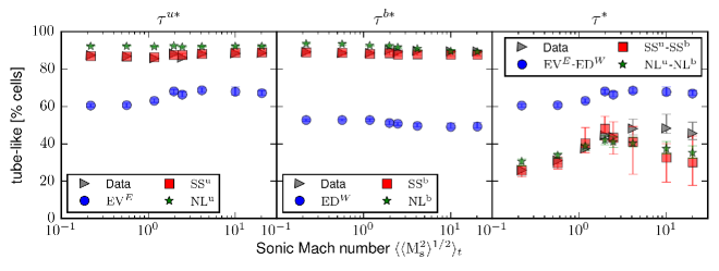
Figure 8: Topology of deviatoric stress tensors by mean percentage of tube-like structures over all snapshots of each simulation (1, 2a, 4, 6, 7a, 11, 12 and 13, see table 1). The remaining structures are sheet-like. The error bars indicate the minimum and maximum value over time for each simulation.

We begin our structural analysis with the comparison of the deviatoric stress tensor topology. Figure 8 illustrates the amount of tube-like structures in our simulations. The only other possibility for $\tau^{\mathrm{u}*}$, $\tau^{\mathrm{b}*}$ and $\tau^{*}$ are sheet-like structures. Analyzing the kinetic $\tau^{\mathrm{u}*}$ and magnetic $\tau^{\mathrm{b}*}$ tensors individually we have $\approx 88\%$ tube-like structures and $\approx 12\%$ sheet-like structures in the data independent of tensor and sonic Mach number $\mathrm{M_{s}}$. Furthermore, there are almost no temporal variations within each simulation – the error bars indicating the minimum and maximum are within the markers. The scale-similarity closures $\mathrm{SS}^{\mathrm{u}}$ and $\mathrm{SS}^{\mathrm{b}}$ match these topologies very closely with differences of only $\approx 1\%$. The nonlinear closures $\mathrm{NL^{u}}$ and $\mathrm{NL^{b}}$ are closely following the data topology as well, even though they slightly overestimate the amount of tube-like structure by $\approx 3\%$ in general. Eddy-viscosity $\mathrm{EV}^{E}$ and eddy-diffusivity $\mathrm{ED}^{W}$ closures on the other hand are not able to match the flow topology. While $\mathrm{EV}^{E}$ is able to reproduce at least the correct tendency with dominating tube structures ($65\%$), $\mathrm{ED}^{W}$ produces an equal share of tube and sheet structures. Interestingly, the topological configuration changes dramatically when analyzing the deviatoric tensor $\tau^{*}=\tau^{\mathrm{u}*}-\tau^{\mathrm{b}*}$ as a whole. The dominant, $\mathrm{M_{s}}$-independent tube-like topology vanishes and sheet configurations become dominant in the subsonic regime. In the supersonic regime tube- and sheet-like configurations are equally present with some (<$10\%$) temporal variation. Again, scale-similarity and nonlinear closures are able to follow the trend more closely than eddy-dissipation type closures. $\mathrm{EV}^{E}$-$\mathrm{ED}^{W}$ exhibits the same behavior as $\mathrm{EV}^{E}$ alone and provides mainly tube-like topology. The scale-similarity closure correctly captures the topology in the subsonic regime with negligible temporal variations. However, in the supersonic regime the amount of sheet-like structures is overestimated by $15\%$ on average and there are temporal variations of up to $14\%$. In contrast to this, the nonlinear closure shows less variations (<$4\%$). However, it also overestimates sheet-like structure in the supersonic regime, but by only $10\%$. Overall these results are in line with the original closure approaches – functional versus structural. The functional eddy-dissipation closures do not perform well in this structural test, whereas both structural closure families are capable of capturing the data topology.

IV.5 Structural analysis: alignment and magnitude

In order to asses how the different closures perform as vectors in the equations, i.e. $\nabla\cdot\widehat{\tau}$ and $\nabla\times\widehat{\bm{\mathcal{E}}}$, we compare their magnitude and alignment with the reference data.

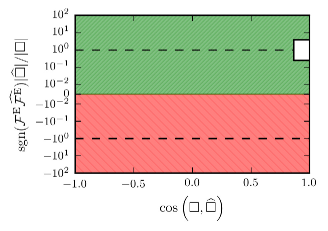
Figure 9: Illustration of magnitude-alignment 2D-histograms (see figure 10). The x-axis shows the alignment between closure vector and reference vector. Relative closure magnitudes are given on the y-axis with the dashed (- -) lines indicating identical closure and reference magnitude. The upper half (green “/” hatching) indicates equal direction in energy cascade, i.e. same sign of $\mathcal{F}^{E}$ and $\widehat{\mathcal{F}^{E}}$, whereas the lower half (red “\” hatching) corresponds to opposed directions. The white box illustrates the area of optimal performance: alignment is within $30^{\circ}$, relative magnitude within a factor of 4, and identical flux sign.

Figure 9 is an explanatory sketch of the 2D-histograms we use for the analysis. The relative vector magnitude, e.g. $|\nabla\cdot\widehat{\tau}_{ij}^{\mathrm{u}*}|/|\nabla\cdot\tau^{\mathrm{u}*}|$, is plotted against the angle between closure and exact solution, e.g. $\cos\left(\nabla\cdot\widehat{\tau}_{ij}^{\mathrm{u}*},\nabla\cdot\tau^{\mathrm{u}*}\right)$. Furthermore, we use the sign of the product of closure flux $\widehat{\mathcal{F}^{E}}$ and reference flux $\mathcal{F}^{E}$ to split the histogram in two halves. A positive sign corresponds to the right direction of the cascade, while a negative one indicates opposite direction. We choose this kind of presentation as it illustrates several independent measures for single-coefficient closures. Firstly, the magnitude is a direct result of the free coefficient value that is determined by the fitting process. Secondly, the sign of the fluxes is determined in conjunction with a resolved flow quantity, e.g. $\widetilde{\bm{u}}$ for $\mathcal{F}^{E}=\widetilde{\bm{u}}\cdot\left(\nabla\cdot\tau\right)$, see (80), and is independent of the coefficient magnitude. Thirdly, the angle is given by the SGS terms alone and is also independent of the coefficient magnitude. We define a region of optimal performance in order to make quantitative statements. Within this region the relative magnitude does not deviate by more than a factor of 4, the angle between closure and data is <$30^{\circ}$, and both fluxes ($\widehat{\mathcal{F}^{E}}$ and $\mathcal{F}^{E}$) have identical sign. We use the results of the energy flux fits $\mathcal{F}^{E}$ in this subsection. Nevertheless, we also verified that the conclusions similarly apply to the other flux fits $\Sigma^{E}$, $\Sigma^{W}$ and $\mathcal{F}^{W}$.

Figure 10 illustrates the resulting 2D-histograms for the best performing closures in a snapshot of the supersonic simulation 7a at $t=4T$, which has randomly been chosen for illustration purposes.

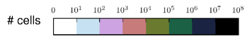
(a) Deviatoric SGS Reynolds stress closures $\widehat{\tau}_{ij}^{\mathrm{u}*}$

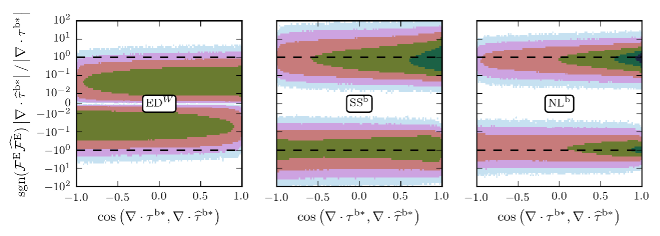
(b) Deviatoric SGS Maxwell stress closures $\widehat{\tau}_{ij}^{\mathrm{b}*}$

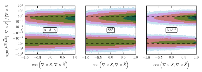
(c) Electromotive force closures $\widehat{\bm{\mathcal{E}}}$

Figure 10: Two dimensional histograms showing the distribution of relative closure vector magnitude, i.e. $\operatorname{sgn}\left(\mathcal{F}^{E}\widehat{\mathcal{F}}^{E}\right)|\nabla\cdot\widehat{\tau}^{\mathrm{u}*}|/|\nabla\cdot\tau^{\mathrm{u}*}|$, versus alignment, i.e. $\cos\left(\nabla\cdot\widehat{\tau}^{\mathrm{u}*},\nabla\cdot\tau^{\mathrm{u}*}\right)$, between closure and data vector. The additional signum, $\operatorname{sgn}$, function on the y-axis is used to indicate flux alignment, i.e. whether data flux $\mathcal{F}^{E}$ and the flux predicted by the closure $\widehat{\mathcal{F}}^{E}$ have identical sign. Dashed lines in each plot illustrate identical closure and data vector magnitudes. The data is taken from a single snapshot at $t=4T$ of supersonic simulation 7a filtered at $k=16$.

The deviatoric SGS Reynolds stress $\widehat{\tau}_{ij}^{\mathrm{u}*}$ closures $\mathrm{EV}^{E}$, $\mathrm{SS}^{\mathrm{u}}$ and $\mathrm{NL^{u}}$ are shown in figure 10(a). In general, the magnitude predicted by $\mathrm{EV}^{E}$ and $\mathrm{SS}^{\mathrm{u}}$ is too small. Furthermore, the angle between closure and data is almost randomly distributed with a slight tendency of alignment, which is more pronounced for $\mathrm{SS}^{\mathrm{u}}$. In contrast to this, $\mathrm{NL^{u}}$ exhibits a clear peak at exact alignment and equal magnitude.

Over all simulations $49^{+10}_{-4}\%$ (median and bounds giving the maximum and minimum) of the cells within the simulation cube are within the region of optimal performance for $\mathrm{NL^{u}}$ and $81^{+3}_{-2}\%$ have the correct sign of $\mathcal{F}^{E}$. $\mathrm{SS}^{\mathrm{u}}$ has still $66^{+2}_{-2}\%$ cells with the correct sign and $14^{+4}_{-3}\%$ in the optimal region, whereas $\mathrm{EV}^{E}$ performs worst with $5^{+4}_{-4}\%$ in the optimal region and only $58^{+2}_{-2}\%$ with equal sign.

Figure 10(b) illustrates the deviatoric SGS Maxwell closures $\mathrm{NL^{b}}$, $\mathrm{SS}^{\mathrm{b}}$ and $\mathrm{ED}^{W}$ for the same snapshot. Overall, the nonlinear and scale-similarity closure behave very similar to their kinetic counterparts with $61^{+13}_{-12}\%$ optimal region and $84^{+5}_{-5}\%$ correct sign for $\mathrm{NL^{b}}$, and $27^{+5}_{-8}\%$ optimal region and $71^{+3}_{-2}\%$ correct sign for $\mathrm{SS}^{\mathrm{b}}$, respectively. The weak performance of eddy-diffusivity closures described in the previous section is also apparent here. The magnitude of $\mathrm{ED}^{W}$ is typically too small by more than a factor of 10. This comes as no surprise as it is determined by the free coefficient. Given that $\mathcal{F}^{E}$ and $\widehat{\mathcal{F}^{E}}$ have matching signs only in $52^{+1}_{-1}\%$ of the cells, which corresponds to random behavior, the fitting process favors a closure close to $0$. In addition to this, the distribution of the angle between closure and data, which is independent of the fitting procedure, is completely random and <$1\permil$ are in the optimal region.

Finally, the EMF closures $\alpha\text{-}\beta\text{-}\gamma$, $\mathrm{SS}^{\mathcal{E}}$ and $\mathrm{NL}^{\mathcal{E},\rho}$ are depicted in figure 10(c) for the same snapshot. Here, the performance of the eddy-dissipation family closure $\alpha\text{-}\beta\text{-}\gamma$ is best compared to the other terms. Overall, $13^{+4}_{-4}\%$ cells are within the optimal region and $61^{+5}_{-4}\%$ have the correct sign. $\mathrm{SS}^{\mathcal{E}}$ performs slightly better with $19^{+4}_{-7}\%$ and $66^{+2}_{-5}\%$, respectively. In both cases the closure vector is more likely to be aligned with the data vector even though it is not as pronounced as for the $\mathrm{NL}^{\mathcal{E},\rho}$ closure. For the nonlinear closure $53^{+6}_{-29}\%$ are within the optimal region whereby the lower limit stems from the highly supersonic simulations 12 and 13. Nevertheless, $\mathrm{NL}^{\mathcal{E},\rho}$ produces the correct flux sign in the majority of cells ($80^{+3}_{-8}\%$) and the variation is less extensive.

The general trend that nonlinear closures are performing best, followed by scale-similarity closures and eventually eddy-dissipation closures is again visible for all terms, $\tau^{\mathrm{u}*}$, $\tau^{\mathrm{b}*}$ and ${\bm{\mathcal{E}}}$.

V Conclusions and outlook

In this paper we systematically conducted a priori tests of different subgrid-scale closures in the realm of compressible magnetohydrodynamics. Over a large parameter space of 15 simulations of forced, homogeneous, isotropic turbulence with sonic Mach numbers ranging from $\mathrm{M_{s}}=0.2$ to $20$ we were able to show that closures of the proposed nonlinear type outperform traditional closures of eddy-dissipation and scale-similarity type in every single test. The main feature of the nonlinear closures is that they require no assumptions about the nature of the flow or turbulence, and, therefore, are able to capture anisotropic effects and support up- and down-scale energy transfer. In contrast, the scale-similarity and eddy-dissipation type closures assume some universal behavior of turbulence. The a priori tests included the correlation between closure and explicitly filtered reference data for quantities such as the turbulent energy $\Sigma^{E}$ and cross-helicity $\Sigma^{W}$ cascades, and total turbulent energy $\mathcal{F}^{E}$ and cross-helicity $\mathcal{F}^{W}$ fluxes. The turbulent energy cascade flux has also been used to analyze the average SGS dissipation. Additionally, we also evaluated the distribution of topological structures for the SGS Reynolds and Maxwell stress tensors and their alignment with respect to the reference data in physical space. Moreover, we verified that our conclusions are not sensitive to resolution, filter width or filter kernel by comparing results between $512^{3}$ and $1024^{3}$ resolution simulations at filter widths of $k=4,8,16,32,64$ with box kernel and a Gaussian kernel. Finally, we were able to verify that the free coefficients of the basic nonlinear closures are very close to unity as expected from the analytic derivation.

Overall, we conclude that the eddy-dissipation family including the popular Smagorinsky closure has only a limited range of applicability, e.g. in situations with dominantly supersonic turbulence and in situations where local flow features are less important. Closures of the scale-similarity family or the nonlinear family can be applied in much more diverse situations, e.g. where anisotropic features or up-scale energy transfer are required. However, there is still room for improvement as the net up-scale transfer via the SGS Maxwell stress is overestimated. Furthermore, the scale-similarity closures should be handled with care as their performance varies strongly with reference quantity and sonic Mach number. The basic nonlinear closures, $\mathrm{NL^{u}}$, $\mathrm{NL^{b}}$ and $\mathrm{NL}^{\mathcal{E},\rho}$, on the other hand perform well across the entire parameter space and are able to reproduce local flow features.

This encourages the application of the basic nonlinear closures as a zero-coefficient SGS model in large-eddy simulations of compressible MHD. These simulations would benefit from the additional physics provided by the SGS model. Promising processes for such LES are turbulent magnetic reconnectionOishi et al. (2015) or the turbulent dynamoSchober et al. (2015), for example, in star-forming magnetized cloudsMac Low and Klessen (2004) or even in galaxiesPakmor, Marinacci, and Springel (2014) and clusters.

References

References

- Cooper et al. (2014) C. M. Cooper, J. Wallace, M. Brookhart, M. Clark, C. Collins, W. X. Ding, K. Flanagan, I. Khalzov, Y. Li, J. Milhone, M. Nornberg, P. Nonn, D. Weisberg, D. G. Whyte, E. Zweibel, and C. B. Forest, Physics of Plasmas 21, 013505 (2014).
- Oishi et al. (2015) J. S. Oishi, M.-M. Mac Low, D. C. Collins, and M. Tamura, ApJ 806, L12 (2015), arXiv:1505.04653 [astro-ph.SR] .
- Schober et al. (2015) J. Schober, D. R. G. Schleicher, C. Federrath, S. Bovino, and R. S. Klessen, Phys. Rev. E 92, 023010 (2015).
- Goldstein, Roberts, and Matthaeus (1995) M. L. Goldstein, D. A. Roberts, and W. H. Matthaeus, ARA&A 33, 283 (1995).
- Balbus and Hawley (1998) S. A. Balbus and J. F. Hawley, Rev. Mod. Phys. 70, 1 (1998).
- Schmidt (2015) W. Schmidt, Living Reviews in Computational Astrophysics 1 (2015), 10.1007/lrca-2015-2.
- Miesch et al. (2015) M. Miesch, W. Matthaeus, A. Brandenburg, A. Petrosyan, A. Pouquet, C. Cambon, F. Jenko, D. Uzdensky, J. Stone, S. Tobias, J. Toomre, and M. Velli, Space Science Reviews , 1 (2015).
- Chernyshov, Karelsky, and Petrosyan (2014) A. A. Chernyshov, K. V. Karelsky, and A. S. Petrosyan, Physics-Uspekhi 57, 421 (2014).
- Vlaykov (2015) D. G. Vlaykov, Sub-grid Scale Modelling of Compressible Magnetohydrodynamic Turbulence: Derivation and A Priori Analysis, Ph.D. thesis, Georg-August University School of Science (GAUSS) Göttingen (2015).
- Favre (1983) A. Favre, Physics of Fluids 26, 2851 (1983).
- Sagaut (2006) P. Sagaut, Large Eddy Simulation for Incompressible Flows: An Introduction, Scientific Computation (Springer, 2006).
- Lu and Porté-Agel (2010) H. Lu and F. Porté-Agel, Physics of Fluids 22, 015109 (2010), http://dx.doi.org/10.1063/1.3291073.
- VREMAN, GEURTS, and KUERTEN (1997) B. VREMAN, B. GEURTS, and H. KUERTEN, Journal of Fluid Mechanics 339, 357 (1997).
- Balarac et al. (2013) G. Balarac, J. Le Sommer, X. Meunier, and A. Vollant, Physics of Fluids 25, 075107 (2013), http://dx.doi.org/10.1063/1.4813812.
- Braun et al. (2014) H. Braun, W. Schmidt, J. C. Niemeyer, and A. S. Almgren, Monthly Notices of the Royal Astronomical Society 442, 3407 (2014).
- Latif et al. (2013) M. A. Latif, D. R. G. Schleicher, W. Schmidt, and J. C. Niemeyer, Monthly Notices of the Royal Astronomical Society 436, 2989 (2013).
- Miki and Menon (2008) K. Miki and S. Menon, Physics of Plasmas (1994-present) 15, 072306 (2008).
- Theobald, Fox, and Sofia (1994) M. L. Theobald, P. A. Fox, and S. Sofia, Physics of Plasmas 1, 3016 (1994).
- Müller and Carati (2002) W.-C. Müller and D. Carati, Physics of Plasmas (1994-present) 9, 824 (2002).
- Yokoi (2013) N. Yokoi, Geophys. Astrophys. Fluid Dyn. , 37 (2013).
- Balarac et al. (2010) G. Balarac, A. G. Kosovichev, O. Brugière, A. A. Wray, and N. N. Mansour, in Proceedings of the Summer Program (Center for Turbulence Research, Stanford University/NASA, 2010) pp. 503–512.
- Grete et al. (2015) P. Grete, D. G. Vlaykov, W. Schmidt, D. R. G. Schleicher, and C. Federrath, New Journal of Physics 17, 023070 (2015).
- Vlaykov et al. (2016) D. G. Vlaykov, P. Grete, W. Schmidt, and D. R. G. Schleicher, to be published in Physics of Plasmas (2016).
- Smagorinsky (1963) J. Smagorinsky, Monthly Weather Review 91, 99 (1963).
- Vreman, Geurts, and Kuerten (1994) B. Vreman, B. Geurts, and H. Kuerten, Journal of Fluid Mechanics 278, 351 (1994).
- Agullo et al. (2001) O. Agullo, W.-C. Müller, B. Knaepen, and D. Carati, Physics of Plasmas 8, 3502 (2001).
- Widmer, Büchner, and Yokoi (2015) F. Widmer, J. Büchner, and N. Yokoi, ArXiv e-prints (2015), arXiv:1511.04347 [physics.plasm-ph] .
- Bardina, Ferziger, and Reynolds (1980) J. Bardina, J. H. Ferziger, and W. C. Reynolds, eds., American Institute of Aeronautics and Astronautics, Fluid and Plasma Dynamics Conference, 13th, Snowmass, Colo., July 14-16, 1980, 10 p. (1980).
- Liu, Meneveau, and Katz (1994) S. Liu, C. Meneveau, and J. Katz, Journal of Fluid Mechanics 275, 83 (1994).
- Leonard (1975) A. Leonard, in Turbulent Diffusion in Environmental PollutionProceedings of a Symposium held at Charlottesville, Advances in Geophysics, Vol. 18, Part A, edited by F. Frenkiel and R. Munn (Elsevier, 1975) pp. 237 – 248.
- Yeo (1987) W. K. Yeo, A generalized high pass/low pass averaging procedure for deriving and solving turbulent flow equations, Ph.D. thesis, The Ohio State University (1987).
- Woodward et al. (2006) P. R. Woodward, D. H. Porter, S. Anderson, T. Fuchs, and F. Herwig, Journal of Physics Conference Series 46, 370 (2006).
- Schmidt and Federrath (2011) W. Schmidt and C. Federrath, Astron. Astrophys. 528, A106 (2011).
- Bryan et al. (2014) G. L. Bryan, M. L. Norman, B. W. O’Shea, T. Abel, J. H. Wise, M. J. Turk, D. R. Reynolds, D. C. Collins, P. Wang, S. W. Skillman, B. Smith, R. P. Harkness, J. Bordner, J. hoon Kim, M. Kuhlen, H. Xu, N. Goldbaum, C. Hummels, A. G. Kritsuk, E. Tasker, S. Skory, C. M. Simpson, O. Hahn, J. S. Oishi, G. C. So, F. Zhao, R. Cen, Y. Li, and T. E. Collaboration, The Astrophysical Journal Supplement Series 211, 19 (2014).
- Fryxell et al. (2000) B. Fryxell, K. Olson, P. Ricker, F. X. Timmes, M. Zingale, D. Q. Lamb, P. MacNeice, R. Rosner, J. W. Truran, and H. Tufo, Astrophys. J. Suppl. Ser. 131, 273 (2000).
- Pope (2000) S. B. Pope, Turbulent Flows (Cambridge University Press, 2000) cambridge Books Online.
- Schmidt et al. (2009) W. Schmidt, C. Federrath, M. Hupp, S. Kern, and J. C. Niemeyer, Astronomy & Astrophysics 494, 127 (2009).
- Federrath et al. (2010) C. Federrath, J. Roman-Duval, R. S. Klessen, W. Schmidt, and M.-M. Mac Low, A&A 512, A81 (2010).
- Toro (2009) E. F. Toro, Riemann solvers and numerical methods for fluid dynamics: a practical introduction (Springer Science & Business Media, 2009).
- Miyoshi and Kusano (2005) T. Miyoshi and K. Kusano, Journal of Computational Physics 208, 315 (2005).
- Federrath et al. (2011) C. Federrath, G. Chabrier, J. Schober, R. Banerjee, R. S. Klessen, and D. R. G. Schleicher, Phys. Rev. Lett. 107, 114504 (2011).
- Federrath et al. (2014) C. Federrath, J. Schober, S. Bovino, and D. R. G. Schleicher, Astrophys. J. 797, L19 (2014).
- Waagan, Federrath, and Klingenberg (2011) K. Waagan, C. Federrath, and C. Klingenberg, Journal of Computational Physics 230, 3331 (2011).
- Dedner et al. (2002) A. Dedner, F. Kemm, D. Kröner, C.-D. Munz, T. Schnitzer, and M. Wesenberg, Journal of Computational Physics 175, 645 (2002).
- Kitsionas et al. (2009) S. Kitsionas, C. Federrath, R. S. Klessen, W. Schmidt, D. J. Price, L. J. Dursi, M. Gritschneder, S. Walch, R. Piontek, J. Kim, A.-K. Jappsen, P. Ciecielag, and M.-M. Mac Low, Astron. Astrophys. 508, 541 (2009).
- Newville et al. (2014) M. Newville, T. Stensitzki, D. B. Allen, and A. Ingargiola, “LMFIT: Non-Linear Least-Square Minimization and Curve-Fitting for Python,” (2014).
- Dallas and Alexakis (2013) V. Dallas and A. Alexakis, Phys. Fluids 25, 105106 (2013), arXiv:1304.0695 .
- (48) See supplemental material at [URL will be inserted by AIP] for detailed correlation and coefficient values split by simulation.
- Mac Low and Klessen (2004) M.-M. Mac Low and R. S. Klessen, Reviews of Modern Physics 76, 125 (2004).
- Pakmor, Marinacci, and Springel (2014) R. Pakmor, F. Marinacci, and V. Springel, The Astrophysical Journal Letters 783, L20 (2014).