The distribution of first hitting times of random walks on Erdős-Rényi networks

Abstract

Analytical results for the distribution of first hitting times of random walks on Erdős-Rényi networks are presented. Starting from a random initial node, a random walker hops between adjacent nodes until it hits a node which it has already visited before. At this point, the path terminates. The path length, namely the number of steps, $d$, pursued by the random walker from the initial node up to its termination is called the first hitting time or the first intersection length. Using recursion equations, we obtain analytical results for the tail distribution of the path lengths, $P(d>\ell)$. The results are found to be in excellent agreement with numerical simulations. It is found that the distribution $P(d>\ell)$ follows a product of an exponential distribution and a Rayleigh distribution. The mean, median and standard deviation of this distribution are also calculated, in terms of the network size and its mean degree. The termination of an RW path may take place either by backtracking to the previous node or by retracing of its path, namely stepping into a node which has been visited two or more time steps earlier. We obtain analytical results for the probabilities, $p_{b}$ and $p_{r}$, that the cause of termination will be backtracking or retracing, respectively. It is shown that in dilute networks the dominant termination scenario is backtracking while in dense networks most paths terminate by retracing. We also obtain expressions for the conditional distributions $P(d=\ell|b)$ and $P(d=\ell|r)$, for those paths which are terminated by backtracking or by retracing, respectively. These results provide useful insight into the general problem of survival analysis and the statistics of mortality rates when two or more termination scenarios coexist.

Keywords: Random network, Erdős-Rényi network, degree distribution, random walk, self-avoiding walk, first hitting time, first intersection length.

1 Introduction

Random walk (RW) models [1, 2] are useful for the study of a large variety of stochastic processes such as diffusion [3, 4], polymer structure [5, 6], and random search [7, 8]. These models were studied extensively in different geometries, including continuous space [9], regular lattices [10], fractals [11] and random networks [12]. In the context of complex networks [13, 14], random walks can be used for either probing the network structure itself [15] or to model dynamical processes such as the spreading of rumors, opinions and epidemics [16, 17].

A RW on a network hops randomly at each time step to one of the nodes which are adjacent to the current node. Thus, if the current node is of degree $k$, the probability of each one of its neighbors to be selected by the RW is $1/k$. Starting from a random initial node, $x_{0}$, the RW generates a path of the form $x_{0}\rightarrow x_{1}\rightarrow\dots\rightarrow x_{t}\rightarrow\dots$, consisting of the nodes it has visited. In some of the steps it hops into new nodes which have not been visited before. In other steps it hops into previously visited nodes, forming loops in its path. The number of distinct nodes visited up to time $t$ is thus typically smaller than $t$. The scaling of the mean number of distinct nodes, $s(t)$, visited by a RW on a random network after $t$ steps was recently studied [18]. It was found that for an infinite network $s(t)\simeq rt$, where $r<1$ is a prefactor which depends on the network topology. These scaling properties resemble those obtained for RWs on high dimensional lattices. In particular, it was found that RWs on random networks are highly effective in exploring the network, retracing their steps much less frequently than RWs on low dimensional lattices [19]. In the case of finite networks, another interesting quantity which appears, is the mean cover time, namely the average number of steps required for the RW to visit all the nodes in the network [20]. Unlike regular lattices, on a complex network of a finite size, the rates in which the RW visits different nodes are not identical, but may depend on the degree of the node, its location in the network and on various correlations between adjacent nodes. In a random, undirected network which exhibits no correlations, such as the Erdős-Rényi (ER) network, the rate in which nodes of degree $k$ are visited, is linearly proportional to $k$. RWs on random networks also give rise to various first passage problems [21]. An interesting example is the mean trapping time, namely the average number of steps required for a RW in order to reach a specific node from a random initial node [22].

A special type of random walk, which has been studied extensively on regular lattices, is the self avoiding walk (SAW). This is a random walk which does not visit the same node more than once [23]. At each time step, the walker chooses its next move randomly from the neighbors of its present node, excluding nodes which were already visited [24, 25, 26, 27, 28, 29, 30]. The path terminates when the SAW reaches a stalemate situation, namely a dead end node which does not have any yet unvisited neighbors. The path length, $d$, is given by the number of steps made by the RW until it was terminated. The path length of an SAW on a connected network of size $N$ can take values between $1$ and $N-1$. The latter case corresponds to a Hamiltonian path [31]. More specifically, the SAW path lengths between a given pair of nodes, $i$ and $j$, are distributed in the range bounded from below by the shortest path length between these nodes [32, 33] and from above by the longest non-overlapping path between them [34]. From a theoretical point of view, the SAW path length corresponds to the attrition length [35]. Using time units rather than length units, we also refer to the path lengths of SAWs as last hitting times.

In a recent paper [36] we obtained analytical results for the distribution of SAW path lengths, or last hitting times, on ER networks [37, 38, 39]. These SAW paths are often referred to as kinetic growth self-avoiding walks [40], or true self avoiding walks [41]. This is in contrast to the SAW paths which are uniformly sampled among all possible self avoiding paths of a given length. It was found that the distribution of path lengths follows the Gompertz distribution [42, 43, 44, 45]. This means that the SAWs exhibit a termination rate per step which increases exponentially with the number of steps already pursued. In the limit of dilute networks it was found that the probability density function of the path lengths, $P(d=\ell)$, is a monotonically decreasing function and most paths are short. As the connectivity of the network is increased, the paths become longer and the path length distribution develops a peak. Further increase in the connectivity shifts the peak to the right. We derived analytical expressions for several central measures (mean, median and mode) and for dispersion measures (standard deviation and the interquartile range) of this distribution.

Another important time scale which appears in random walks on networks is the first hitting time [18], also referred to as the first intersection length [46, 47]. This time scale emerges in a class of RW models which are not restricted to be self avoiding. In these models the RW keeps hopping between adjacent nodes until it enters a node which it has already visited before. At this point the path is terminated. The number of time steps up to the termination of the path, which coincides with the path length, is called the first hitting time. For a given network size, the first hitting time tends to increase as the network becomes more strongly connected, because as the degree of a node is increased it takes longer for the RW to visit a given fraction of its neighbors. However, it is always much smaller than the last hitting time, namely the length of the corresponding SAW path. This is due to the fact that the RW may be terminated at any time step $t>1$ by randomly hopping into an already visited node, even if the current node has one or more yet-unvisited neighbors, while the SAW terminates only when the current node does not have any yet-unvisited neighbors.

A RW model which terminates at its first hitting time can be cast in the language of foraging theory as a model describing a wild animal, which is randomly foraging in a random network environment. Each time the animal visits a node it consumes all the food available in this node and needs to move on to one of the adjacent nodes. The model describes rather harsh conditions, in which the regeneration of resources is very slow and the visited nodes do not replenish within the lifetime of the forager. Moreover, the forager does not carry any reserves and in order to survive it must hit a vital node each and every time. More realistic variants of this model have been studied on lattices of different dimensions. It was shown that under slow regeneration rates, the forager is still susceptible to starvation, while above some threshold regeneration rate, the probability of starvation diminishes [48]. The case in which the forager carries sufficient resources that enable it to avoid starvation even when it visits up to $S$ non-replenished nodes in a row, was also studied [49, 50].

In this paper we present analytical results for the distribution $P(d=\ell)$ of first hitting times of RWs on an ensemble of ER networks. In our analysis, we utilize the fact that up to its termination the RW follows an SAW path. The path pursued by the RW may terminate either by backtracking into the previous node or by retracing itself, namely stepping into a node which was already visited two or more time steps earlier. By calculating the probabilities of these two scenarios, we obtain analytical results for the distribution of the first hitting times of RWs on ER networks. The results are found to be in excellent agreement with numerical simulations. We obtain analytical results for the overall probabilities, $p_{b}$ and $p_{r}$, that a RW, starting from a random initial node, will be terminated by backtracking or by retracing, respectively. It is found that in dilute networks most paths are terminated by backtracking while in dense networks most paths are terminated by retracing. We also obtain expressions for the conditional distributions of path lengths, $P(d=\ell|b)$ and $P(d=\ell|r)$ for the RWs which are terminated by backtracking or by retracing, respectively. These results provide useful insight into the general problem of survival analysis and the statistics of mortality or failure rates, under conditions in which two or more failure mechanisms coexist [51, 52].

The paper is organized as follows. In Sec. 2 we describe the random walk model on an ER network. In Sec. 3 we briefly describe some properties of the ER network which are important for the analysis presented in this paper. In Sec. 4 we consider the temporal evolution of two subnetworks, one consisting of the nodes already visited by the RW and the other consisting of the yet unvisited nodes. In Sec. 5 we derive analytical results for the distribution of first hitting times of RWs on ER networks. In Sec. 6 we obtain analytical expressions for two central measures (mean and median) and for a dispersion measure (the standard deviaion) of this distribution. In Sec. 7 we calculate the termination probabilities by the backtracking and by the retracing mechanisms. We also calculate the conditional path length distributions for RWs which terminate by each one of these two mechanisms. The results are summarized and discussed in Sec. 8.

2 The random walk model

Consider a RW on a random network of $N$ nodes. Each time step the walker chooses randomly one of the neighbors of its current node, and hops to the chosen node. Here we study the case in which the RW path is terminated upon the first time it steps into an already visited node. The resulting path length, $d$, namely the number of steps pursued by the RW until its termination, is referred to as the first hitting time or as the first intersection length. In the analysis below we do not include the termination step itself as a part of the RW path. This means that the path length of a RW which pursued $\ell$ steps and was terminated in the $\ell+1$ step, is $d=\ell$. The path includes $\ell+1$ nodes, since the initial node is also counted as a part of the path. Interestingly, the paths of the RWs up to the termination step are, in fact, SAW paths, since each node along the path is visited only once. The termination may take place in two possible ways. In one scenario the path is terminated when the RW backtracks into the previous node, while in the other scenario it steps into a node which was already visited at an earlier time.

3 The Erdős-Rényi network

In this section we briefly summarize the properties of ER networks which are of particular relevance to the analysis presented below. The ER network is the simplest model of a random network [37, 38, 39]. It has been studied extensively over more than five decades and many of its properties are known exactly [31]. The ER network, denoted by $ER(N,p)$, consists of $N$ nodes such that each pair of nodes is connected with probability $p$. The degree distribution of an ER network is a binomial distribution, $B(N,p)$. In the limit $N\rightarrow\infty$ and $p\rightarrow 0$, where the mean degree $c=(N-1)p$ is held fixed, it converges to a Poisson distribution of the form

$$p_{0}(k)=\frac{{c}^{k}}{k!}e^{-c}.$$ (1)

Clearly, there are no degree-degree correlations between adjacent nodes. In fact, ER networks can be considered as a maximum entropy ensemble under the constraint that the mean degree is fixed. In the asymptotic limit ($N\rightarrow\infty$), the ER network exhibits a phase transition at $c=1$ (a percolation transition), such that for $c<1$ the network consists only of small clusters and isolated nodes, while for $c>1$ there is a giant cluster which includes a macroscopic fraction of the network, in addition to the small clusters and isolated nodes. At a higher value of the connectivity, namely at $c=\ln N$, there is a second transition, above which the entire network is included in the giant cluster and there are no isolated components. For intermediate values of $c$, namely for $1<c<\ln N$, the fraction, $g=g(c)$, of nodes which belong to the giant cluster is given by the implicit equation $g=1-\exp(-cg)$. Solving for $g$, one obtains $g(c)=1+{W(-ce^{-c})}/{c}$, where $W(x)$ is the Lambert $W$ function. Thus, the fraction of nodes which belong to network components apart from the giant cluster is given by $1-g$. This includes nodes which reside on small clusters as well as isolated nodes. The fraction, $i=i(c)$, of isolated nodes among all nodes in the network is given by $i(c)=\exp(-c)$. Thus, the fraction, $h=h(c)$, of nodes which reside on isolated clusters of size $s>1$ is given by $h(c)=1-g(c)-i(c)$, or more explicitly by $h(c)=-{W(-ce^{-c})}/{c}-e^{-c}$. Here we focus on the regime above the percolation transition, namely $c>1$. In order to avoid the trivial case of a RW starting on an isolated node, we performed the analysis presented below for the case in which the initial node is non-isolated. However, isolated clusters which consist of two or more nodes are not excluded. Thus, the results presented below correspond to the entire network rather than to the giant component alone.

4 Evolution of the subnetworks of visited and the yet-unvisited nodes

Consider an $ER(N,p)$ network. The degree $k_{i}$ of node $i=1,\dots,N$ is the number of links connected to this node. The RW divides the network into two sub-networks: one consists of the already visited nodes and the other consists of the yet unvisited nodes. After $t$ time steps the size of the subnetwork of visited nodes is $t+1$ (including the initial node), while the size of the network of yet unvisited nodes is $N(t)=N-t-1$. The degree distributions of both sub-networks evolve in time. We denote the degree distribution of the sub-network of the yet unvisited nodes at time $t$ by $p_{t}(k)$, $k=0,\dots,N(t)-1$, where $p_{0}(k)$, is the original degree distribution given by Eq. (1). The mean degree, $c(t)=\langle k\rangle_{t}$, of this sub-network, which is given by

$$c(t)=\sum_{k=0}^{N(t)-1}kp_{t}(k),$$ (2)

evolves accordingly, where $c(0)=c$.

For random walks on random networks, there is a higher probability for the walker to visit nodes with high degrees. More precisely, the probability that in the next time step the RW will visit a node of degree $k$ is $kp_{0}(k)/c$. Conditioned on stepping into one of the yet unvisited nodes adjacent to the current node, the probability of stepping into a node of degree $k$ is $kp_{t}(k)/c(t)$. In Ref. [36] it was shown that for an SAW on an ER network the degree distribution of the subnetwork of the yet unvisited nodes, at time $t$, is

$$p_{t}(k)=\frac{c(t)^{k}}{k!}e^{-c(t)},$$ (3)

where

$$c(t)=c-pt$$ (4)

is the mean degree of this subnetwork. These exact results imply that the subnetwork of the yet unvisited nodes remains an ER network, while its mean degree decreases linearly in time. A special property of the Poisson distribution is that $kp_{t}(k)/c(t)=p_{t}(k-1)$. This means that, the probability that the node visited at time $t+1$ will be of degree $k$ is given by $p_{t}(k-1)$. Since the RW follows an SAW path until it terminates, this result applies also the RW model studied here.

5 The distribution of first hitting times

Consider a RW on an ER network, which starts from a random node with degree $k\geq 1$ (non-isolated node). The RW hops randomly between nearest neighbor nodes. It continues to hop as long as all the nodes it steps into have not been visited before. Once the RW steps into a node which has already been visited, the path is terminated. We distinguish between two termination scenarios. In the first scenario, the RW hops back into the previous node (backtracking step). In the second scenario the RW hops into a node which was already visited at an earlier time (retracing step).

In case that the RW has pursued $t$ steps, without visiting any node more than once, the path length is guaranteed to be $d>t-1$. At this point, the probability that the path will not be terminated in the $t+1$ step is denoted by the conditional probability $P(d>t|d>t-1)$. This conditional probability can be expressed as a product of the form

$$P(d>t|d>t-1)=P_{b}(d>t|d>t-1)P_{r}(d>t|d>t-1).$$ (5)

The conditional probability $P_{b}(d>t|d>t-1)$ is the probability that the RW will not backtrack its path at the $t+1$ time step and will thus avoid the first termination scenario. Given that the RW has not backtracked its path, the conditional probability $P_{r}(d>t|d>t-1)$ is the probability that it will not step into a node already visited at an earlier time, thus avoiding the second termination scenario.

An RW which at time $t$ resides in a node of degree $k$ may hop in the next time step to each one of its $k$ neighbors. One of these neighbors is the previous node, visited by the RW at time $t-1$. Thus, the probability of a backtracking step into the previous node is $1/k$. The degree distribution of nodes visited by an RW is given by $kp_{0}(k)/c$. Thus the probability of backtracking is

$$\left\langle\frac{1}{k}\right\rangle=\sum_{k=1}^{N-1}\frac{1}{k}\frac{kp_{0}(k)}{c}.$$ (6)

Evaluation of the right hand side yields

$$\left\langle\frac{1}{k}\right\rangle=\frac{1-e^{-c}}{c}.$$ (7)

Thus, the probability that the RW will not backtrack its path at time $t+1$ is given by

$$P_{b}(d>t|d>t-1)=1-\left(\frac{1-e^{-c}}{c}\right).$$ (8)

Note that this probability does not depend on $t$.

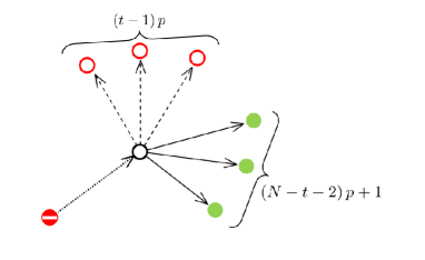
Figure 1: The evaluation of the probability, $P_{r}(d>t|d>t-1)$, that an RW will not terminate by retracing at the $t+1$ time step is illustrated. The total number of neighbors of the current node, apart from the previous node, is $(N-3)p+1$, of which $(N-t-2)p+1$ have not been visited before.

Provided that the RW was not terminated by backtracking at the $t+1$ step, we will now evaluate the probability $P_{r}(d>t|d>t-1)$ that it will also not be terminated by retracing its path in that step. Apart from the current node and the previous node, there are $N-2$ possible nodes which may be connected to the current node, with probability $p$ (Fig. 1). The fact that the possibility of backtracking was already eliminated for the $t+1$ step, guarantees that at least one of these $N-2$ nodes is connected to the current node with probability $1$ (otherwise, the only possible move would have been to hop back to the previous node). This leaves $N-3$ nodes which are connected to the current node with probability $p$. Thus, the expectation value of the number of neighbors of the current node, to which the RW may hop in the $t+1$ step, is $(N-3)p+1$. Due to the local tree-like structure of ER networks, it is extremely unlikely that the one node which is guaranteed to be connected to the current node has already been visited. This is due to the fact that the path from such earlier visit all the way to the current node is essentially a loop. Therefore, we conclude that this adjacent node has not yet been visited. Since the number of yet unvisited nodes is $N-t-1$ we conclude that the current node is expected to have $(N-t-2)p+1$ neighbors which have not yet been visited. As a result, the probability that the RW will hop into one of the yet-unvisited nodes is given by

$$P_{r}(d>t|d>t-1)=\frac{(N-t-2)p+1}{(N-3)p+1}.$$ (9)

Inserting $c=(N-1)p$ and $c(t)=(N-t-1)p$ we obtain

$$P_{r}(d>t|d>t-1)=\frac{c(t)-p+1}{c-2p+1}.$$ (10)

In the asymptotic limit this expression can be approximated by

$$P_{r}(d>t|d>t-1)=\frac{c(t)+1}{c+1}.$$ (11)

Combining the results presented above, it is found that the probability that the RW will proceed from time $t$ to time $t+1$ is given by the conditional probability

$$P(d>t|d>t-1)=\left(\frac{c-1+e^{-c}}{c}\right)\left[\frac{c(t)-p+1}{c-2p+1}\right].$$ (12)

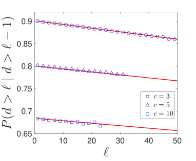
Figure 2: The conditional probability $P(d>\ell|d>\ell-1)$ vs. $\ell$, obtained from Eq. (12) (solid lines) and from numerical simulations of RWs (symbols) on ER networks of size $N=1000$ and mean degrees $c=3$, $5$ and $10$ (squares, triangles and circles, respectively). The analytical and numerical results are found to be in good agreement.

In Fig. 2 we present the conditional probability $P(d>t|d>t-1)$ vs. $t$ for a network of size $N=1000$ and for three values of $c$. The analytical results (solid lines) obtained from Eq. (12) are found to be in good agreement with numerical simulations (symbols), confirming the validity of this equation. Note that the numerical results become more noisy as $t$ increases, due to diminishing statistics, and eventually terminate. This is particularly apparent for the smaller values of $c$.

The probability that the path length of the RW will be longer than $\ell$ is given by

$$P(d>\ell)=P(d>0)\prod_{t=1}^{\ell}P(d>t|d>t-1),$$ (13)

where $P(d>0)=1$, since the initial node is not isolated. Using Eq. (5) the probability $P(d>\ell)$ can be written as a product of the form

$$P(d>\ell)=P_{b}(d>\ell)P_{r}(d>\ell),$$ (14)

where

$$P_{b}(d>\ell)=\prod_{t=1}^{\ell}\left(\frac{c-1+e^{-c}}{c}\right),$$ (15)

and

$$P_{r}(d>\ell)=\prod_{t=2}^{\ell}\left[\frac{c(t)-p+1}{c-2p+1}\right].$$ (16)

The calculation of the tail distribution $P_{b}(d>\ell)$ is simplified by the fact that $P_{b}(d>t|d>t-1)$ does not depend on $t$. As a result, Eq. (15) can be written in the form

$$P_{b}(d>\ell)=e^{-\beta\ell},$$ (17)

where

$$\beta=\ln\left(\frac{c}{c-1+e^{-c}}\right).$$ (18)

Taking the logarithm of $P_{r}(d>\ell)$, as expressed in Eq. (16), we obtain

$$\ln\left[P_{r}(d>\ell)\right]=\sum_{t=2}^{\ell}\ln\left[\frac{c(t)-p+1}{c-2p+1}\right].$$ (19)

Replacing the sum by an integral and plugging in the expression for $c(t)$ from Eq. (4), we obtain

$$\ln[P_{r}(d>\ell)]\simeq\int_{3/2}^{\ell+1/2}\ln\left[1-\frac{c\cdot\left(t-1\right)}{\left(N-1\right)\left(c-2p+1\right)}\right]dt.$$ (20)

The integrand can be simplified by replacing $N-1$ by $N$ and $c-2p+1$ by $c+1$, which is accurate when $p\ll 1$. Using the notation

$$\alpha=\sqrt{\frac{N(c+1)}{c}},$$ (21)

and solving the integral, we obtain

$$\ln[P_{r}(d>\ell)] \simeq \left(\ell-\frac{1}{2}-\alpha^{2}\right)\ln\left[1-\frac{\left(\ell-\frac{1}{2}\right)}{\alpha^{2}}\right]-\ell$$

$$+ \left(\alpha^{2}-\frac{1}{2}\right)\ln\left(1-\frac{1}{2\alpha^{2}}\right)+1.$$

In the approximation of the sum of Eq. (19) by the integral of Eq. (20) we have used the formulation of the middle Riemann sum. Since the function $\ln[P_{r}(d>\ell)]$ is a monotonically decreasing function, the value of the integral is over-estimated by the left Riemann sum, $L_{\alpha}(\ell)$, and under-estimated by the right Riemann sum, $R_{\alpha}(\ell)$. The error involved in this approximation is thus bounded by the difference $\Delta_{\alpha}(\ell)=L_{\alpha}(\ell)-R_{\alpha}(\ell)$, which satisfies $\Delta_{\alpha}(\ell)<\ln(1-\ell/\alpha^{2})$. Thus, the relative error in $P(d>\ell)$ due to the approximation of the sum by an integral is bounded by $\eta_{\rm SI}=\ell/\alpha^{2}$, which scales like $\ell/N$. Comparing the values obtained from the sum and the integral over a broad range of parameters, we find that the pre-factor of the error is very small, so in practice the error introduced by approximation of the sum by an integral is negligible.

Under the assumption that the RW paths are short compared to the network size, namely $\ell\ll N$, one can use the approximation

$$\ln\left(1-\frac{\ell}{\alpha^{2}}\right)\simeq-\frac{\ell}{\alpha^{2}}-\frac{\ell^{2}}{2\alpha^{4}}+O\left(\frac{\ell^{3}}{\alpha^{6}}\right).$$ (23)

Plugging this approximation into Eq. (5) yields

$$P_{r}\left(d>\ell\right)\simeq\exp\left[-\frac{\ell(\ell-1)}{2\alpha^{2}}\right].$$ (24)

Combining the results obtained above for $P_{b}(d>\ell)$ [Eq. (17)] and for $P_{r}(d>\ell)$ [Eq. (24)] we obtain

$$P\left(d>\ell\right)\simeq\exp\left[-\frac{\ell(\ell-1)}{2\alpha^{2}}-\beta\ell\right].$$ (25)

Thus, the distribution of path lengths is a product of an exponential distribution and a Rayleigh distribution, which is a special case of the Weibull distribution [53]. Considering the next order in the series expansion of Eq. (23) we find that the relative error in Eq. (25) for $P(d>\ell)$ due to the truncation of the Taylor expansion after the second order is $\eta_{\rm TE}=\ell^{3}/(6\alpha^{4})$, which scales like $\ell^{3}/N^{2}$. This error is very small as long as $\ell\ll N^{1/2}$. Note that paths of length $\ell\simeq N^{1/2}$, for which the error in $P(d>\ell)$ is noticeable, become prevalent only in the limit of dense networks, where $c>N^{1/2}$.

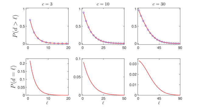
Figure 3: The tail distributions $P(d>\ell)$ vs. $\ell$ of the first hitting times of RWs for ER networks of size $N=1000$ and $c=3$, $10$ and $30$. The theoretical results, obtained from Eq. (25) (solid lines) and the results obtained from numerical simulations (circles) are shown in the top row, and are found to be in excellent agreement with each other. The corresponding probability density functions, $P(d=\ell)$, obtained from Eq. (26), are shown in the bottom row. The agreement with the numerical results is already established in the top row and therefore the numerical data is not shown in the bottom row.

In Fig. 3 we present the tail distributions $P(d>\ell)$ vs. $\ell$ of the first hitting times of RWs on ER networks of size $N=1000$ and mean degrees $c=3$, $10$ and $30$. The theoretical results (solid lines), obtained from Eq. (25), are found to be in excellent agreement with the numerical simulations (symbols). The probability density function $P(d=\ell)$ is given by

$$P\left(d=\ell\right)=P\left(d>\ell-1\right)-P\left(d>\ell\right).$$ (26)

6 Central and dispersion measures of the path length distribution

In order to characterize the distribution of first hitting times of RWs on ER networks we derive expressions for the mean and median of this distribution. The mean of the distribution can be obtained from the tail-sum formula

$$\ell_{\rm mean}(N,c)=1+\sum_{\ell=1}^{N-2}P(d>\ell),$$ (27)

under the assumption that the initial node is a non-isolated node. Expressing the sum as an integral we obtain

$$\ell_{\rm mean}(N,c)=1+\int_{1/2}^{N-3/2}P(d>\ell)d\ell,$$ (28)

where the range of integration is shifted downwards by $1/2$, such that the summation over each integer, $i$, is replaced by an integral over the range $(i-1/2,i+1/2)$. Inserting $P(d>\ell)$ from Eq. (25) and solving the integral, we obtain

$$\ell_{\rm mean}=1+\sqrt{\frac{\pi}{2}}\alpha e^{\frac{(\alpha^{2}\beta-1)\beta}{2}}\left[{\rm erf}\left(\frac{\alpha^{2}\beta+N-2}{\sqrt{2}\alpha}\right)-{\rm erf}\left(\frac{\alpha\beta}{\sqrt{2}}\right)\right].$$ (29)

Using the relative error of Eq. (25) for $P(d>\ell)$, we estimate the relative error of $\ell_{mean}$ by $\eta=\ell_{\rm mean}^{3}/(6\alpha^{4})$, which scales like $\ell_{\rm mean}^{3}/N^{2}$. We can safely approximate the first ${\rm erf}$ on the right hand side of Eq. (29) to be equal to $1$, and obtain

$$\ell_{\rm mean}\simeq 1+\sqrt{\frac{\pi}{2}}\alpha e^{\frac{(\alpha^{2}\beta-1)\beta}{2}}\left[1-{\rm erf}\left(\frac{\alpha\beta}{\sqrt{2}}\right)\right].$$ (30)

In the limit of dense networks, where

$$c>c^{\ast}=\sqrt{\frac{2}{\pi}}\sqrt{N},$$ (31)

$\ell_{\rm mean}$ can be expressed in the asymptotic form

$$\ell_{\rm mean}\simeq 1+\sqrt{\frac{\pi}{2}}\sqrt{N}\left[1-\sqrt{\frac{2}{\pi}}\frac{\sqrt{N}}{c}+\frac{1}{2}\frac{N}{c^{2}}+O\left(\frac{N^{\frac{3}{2}}}{c^{3}}\right)\right].$$ (32)

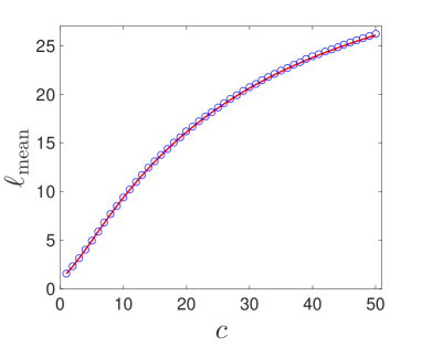
Figure 4: The mean of the distribution of first hitting times, $\ell_{\rm mean}$, as a function of the mean degree, $c$, for ER networks of size $N=1000$. The analytical results (solid line), obtained from Eq. (30) are in excellent agreement with numerical simulations (circles).

In Fig. 4 we present the mean value, $\ell_{\rm mean}$ of the distribution of first hitting times as a function of the mean degree $c$, for ER networks of size $N=1000$. The agreement between the theoretical results, obtained from Eq. (30) and the numerical simulations is very good for all values of $c$.

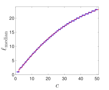
Figure 5: The median of the distribution of first hitting times, $\ell_{\rm median}$, as a function of the mean degree, $c$, for ER networks of size $N=1000$. The analytical results (solid line) are in excellent agreement with numerical simulations (circles).

To obtain a more complete characterization of the distribution of first hitting times, it is also useful to evaluate its median, $\ell_{\rm median}$. Here the median is defined as the value of $\ell$ for which $|P(d>\ell)-P(d<\ell)|\rightarrow{\rm min}$, where $\ell$ may take either an integer or a half-integer value. In Fig. 5 we present the median, $\ell_{\rm median}$, of the distribution of first hitting times as a function of the mean degree, $c$, for ER networks of size $N=1000$. The agreement between the theoretical results and the numerical simulations is very good for all values of $c$. Note that in the evaluation of $\ell_{\rm median}$ we use the accurate expression of $P_{r}(d>\ell)$, given by Eq. (5) rather than the approximate expression of Eq. (24). Using the approximate expression gives rise to small discrepancies in the locations of the edges of the steps for large values of $c$.

In the limit of very high connectivity, Eq. (30) can be approximated by $\ell_{\rm mean}\simeq 1+(\pi N/2)^{1/2}$. Thus, in such dense networks, the mean path length becomes independent of the mean degree $c$, and scales according to $\ell_{\rm mean}\sim\sqrt{N}$. This can be understood as follows. In this limit, the backtracking probability is very low and thus the backtracking-induced termination of paths is no longer of much significance. Instead, retracing becomes the main reason for termination of paths. Due to the very high connectivity, the hopping between adjacent nodes can be considered as the simple combinatorial problem of randomly choosing one node at a time from a set of $N$ nodes, allowing each node to be chosen more than once. The probability that such process will yield $\ell$ distinct nodes is given by $P(d>\ell-2)\simeq\exp(-\ell^{2}/N)$. Thus, in this limit the median is given by $\ell_{\rm median}\simeq\sqrt{N\ln 2}$. This result is analogous to the birthday problem, where $N=365$ and $\ell_{\rm median}$ is the smallest number of participants in a party such that with probability of at least $1/2$ there is at least one pair that has the same birthday [54].

The moments of the distribution of RW path lengths, $\langle\ell^{n}\rangle$, are given by the tail-sum formula [55]

$$\langle\ell^{n}\rangle=\sum_{\ell=0}^{N-1}[(\ell+1)^{n}-\ell^{n}]P(d>\ell).$$ (33)

Using this formula to evaluate the second moment and replacing the sum by an integral we obtain

$$\langle\ell^{2}\rangle=1+\int_{\frac{1}{2}}^{N-\frac{1}{2}}\left(2\ell+1\right)\exp\left[-\frac{\ell(\ell-1)}{2\alpha^{2}}-\beta\ell\right]d\ell.$$ (34)

Solving the integral and taking the large network limit, we obtain

$$\langle\ell^{2}\rangle\simeq 1+2\alpha^{2}e^{-\frac{\beta}{2}}+\sqrt{2\pi}{\alpha}\left(1-\alpha^{2}\beta\right)e^{\frac{(\alpha^{2}\beta-1)\beta}{2}}\left[1-{\rm erf}\left(\frac{\alpha\beta}{\sqrt{2}}\right)\right].$$ (35)

The standard deviation of the distribution of path lengths is thus given by

$$\sigma_{\ell}^{2}(c)=\langle\ell^{2}\rangle-\ell_{mean}^{2},$$ (36)

where $\langle\ell^{2}\rangle$ is given by Eq. (35) and $\ell_{mean}$ is given by Eq. (30). In the dense network limit, where $c>c^{\ast}$, the standard deviation can be approximated by

$$\sigma_{\ell}(c)\simeq\sqrt{\frac{4-\pi}{2}}\sqrt{N}\left[1+\frac{\pi-2}{2c(4-\pi)}-\left(\frac{\pi-2}{4-\pi}\right)\left(\frac{N}{2c^{2}}\right)+O\left(\frac{N^{2}}{c^{3}}\right)\right].$$ (37)

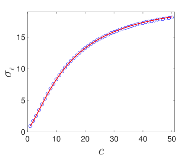
Figure 6: The standard deviation of the distribution of first hitting times, $\sigma_{\ell}$, as a function of the mean degree, $c$, for ER networks of size $N=1000$. The analytical results (solid line), obtained from Eq. (36) are in excellent agreement with numerical simulations (circles).

In Fig. 6 we present the standard deviation, $\sigma_{\ell}(c)$ of the distribution of first hitting times as a function of the mean degree, $c$, for ER networks of size $N=1000$. The agreement between the theoretical results, obtained from Eq. (36), and the numerical simulations is very good for all values of $c$.

7 Analysis of the two termination mechanisms

The RW model studied here may terminate either due to backtracking or due to retracing its path. The backtracking mechanism may occur starting from the second step of the RW. The expected probability of backtracking is $[1-\exp(-c)]/c$ at any step afterwards, regardless of the number of steps already pursued. In case of termination by retracing the RW path forms a loop which starts at the first visit to the termination node and ends in the second visit. Termination due to retracing may play a role starting from the third step of the RW. The probability that the RW will terminate due to retracing increases in time. This is due to the fact that each visited node becomes a potential trap. It is thus expected that paths that terminate after a small number of steps are most likely to be terminated by backtracking, while paths which survive for a long time are more likely to be terminated by retracing. Below we present a detailed analysis of the probabilities of a RW to terminate by backtracking or by retracing. We also present the dependence of these probabilities on the number of steps already pursued.

Consider a RW on an ER network, starting from a random, non-isolated node. The RW will follow a path visiting a new node at each one of the first $\ell$ steps. It will terminate at the $\ell+1$ step, by entering an already visited node. Since the failed termination step is not counted as a part of the path, the path length in this case will be $d=\ell$. The probability distribution function of the RW path lengths, $P(d=\ell)$, is given by Eq. (26). We denote by $p_{b}$ the probability that a RW starting from a random initial node will terminate by backtracking and by $p_{r}$ the probability that it will terminate by retracing. Since these are the only two termination mechanisms in the model, the two probabilities must satisfy $p_{b}+p_{r}=1$.

While the overall distributions of path lengths is given by $P(d=\ell)$, one expects the distribution $P(d=\ell|b)$ of paths terminated by backtracking to differ from the distribution $P(d=\ell|r)$ of paths terminated by retracing. These conditional probability distributions are normalized, namely they satisfy $\sum_{t=2}^{N-1}P(d=t|b)=1$ and $\sum_{t=3}^{N-1}P(d=t|r)=1$. The overall distribution of path lengths can be expressed in terms of the conditional distributions according to

$$P(d=\ell)=p_{b}P(d=\ell|b)+p_{r}P(d=\ell|r).$$ (38)

The first term on the right hand side of Eq. (38) can be written as

$$p_{b}P(d=\ell|b)=P(d>\ell-1)\left[1-P_{b}(d>\ell|d>\ell-1)\right],$$ (39)

namely as the probability that the RW will pursue $\ell$ steps and will terminate in the $\ell+1$ step due to backtracking. The second term on the right hand side of Eq. (38) can be written as

$$p_{r}P(d=\ell|r)=P(d>\ell-1)P_{b}(d>\ell|d>\ell-1)\left[1-P_{r}(d>\ell|d>\ell-1)\right],$$ (40)

namely as the probability that the RW will pursue $\ell$ steps, then in the $\ell+1$ step it will not backtrack its path but will retrace it by stepping into a node visited at least two steps earlier.

Summing up both sides of Eq. (39) over all integer values of $\ell$ we obtain

$$p_{b}=\left(\frac{1-e^{-c}}{c}\right)\sum_{\ell=1}^{N-1}P(d>\ell-1).$$ (41)

Using the tail-sum formula we find that the probability that the RW will terminate by backtracking is

$$p_{b}=\left(\frac{1-e^{-c}}{c}\right)\ell_{\rm mean}.$$ (42)

As a result, the probability of the RW to be terminated by retracing its path is

$$p_{r}=1-\left(\frac{1-e^{-c}}{c}\right)\ell_{\rm mean}.$$ (43)

Using Eq. (39) the conditional probability $P(d=\ell|b)$ can be written in the form

$$P(d=\ell|b)=\frac{P(d>\ell-1)}{\ell_{\rm mean}}.$$ (44)

Similarly, the conditional probability $P(d=\ell|r)$ takes the form

$$P(d=\ell|r)=\left(\frac{c-1+e^{-c}}{c+1}\right)\left[\frac{c-c(\ell)}{c-(1-e^{-c})\ell_{\rm mean}}\right]P(d>\ell-1),$$ (45)

where $c(\ell)$ is given by Eq. (4). The corresponding tail distributions take the form

$$P(d>\ell|b)=\frac{\sum_{t=\ell+1}^{N-1}P(d>t-1)}{\ell_{\rm mean}},$$ (46)

and

$$P(d>\ell|r)=\left(\frac{c-1+e^{-c}}{c+1}\right)\sum_{t=\ell+1}^{N-1}\left[\frac{c-c(t)}{c-(1-e^{-c})\ell_{\rm mean}}\right]P(d>t-1).$$ (47)

Given that a RW path was terminated after $\ell$ steps, it is of great interest to evaluate the conditional probabilities $P(b|d=\ell)$ and $P(r|d=\ell)$, that the termination was caused by backtracking or by retracing, respectively. Using Bayes’ theorem, these probabilities can be expressed by

$$P(b|d=\ell)=\frac{p_{b}P(d=\ell|b)}{P(d=\ell)}$$ (48)

and

$$P(r|d=\ell)=\frac{p_{r}P(d=\ell|r)}{P(d=\ell)}.$$ (49)

Clearly, these distributions satisfy $P(b|d=\ell)+P(r|d=\ell)=1$. Inserting the conditional probabilities $P(d=\ell|b)$ and $P(d=\ell|r)$ from Eqs. (44) and (45), respectively, we find that

$$P(b|d=\ell)=\left(\frac{1-e^{-c}}{c}\right)\frac{P(d>\ell-1)}{P(d=\ell)}$$ (50)

and

$$P(r|d=\ell)=\left(\frac{c-1+e^{-c}}{c+1}\right)\left[1-\frac{c(\ell)}{c}\right]\frac{P(d>\ell-1)}{P(d=\ell)}.$$ (51)

The corresponding tail distributions can be expressed in the form

$$P(b|d>\ell)=\left(\frac{1-e^{-c}}{c}\right)\frac{\sum_{t=\ell+1}^{N-1}P(d>t-1)}{P(d>\ell)}$$ (52)

and

$$P(r|d>\ell)=\left(\frac{c-1+e^{-c}}{c+1}\right)\sum_{t=\ell+1}^{N-1}\left[1-\frac{c(t)}{c}\right]\frac{P(d>t-1)}{P(d>\ell)}.$$ (53)

These distributions also satisfy $P(b|d>\ell)+P(r|d>\ell)=1$.

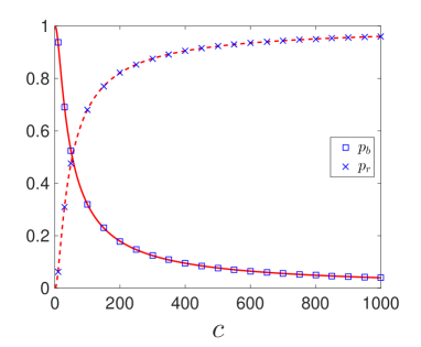
Figure 7: The probabilities $p_{b}$ and $p_{r}$ that a RW on an ER network will terminate via backtracking or by retracing its path, respectively, as a function of the mean degree, $c$. The theoretical results, obtained from Eqs. (42) and (43) are found to be in excellent agreement with the results of numerical simulations (symbols).

In Fig. 7 we present the probability $p_{b}$ that the RW will terminate due to backtracking and the probability $p_{r}$ that it will terminate due to retracing as a function of the mean degree $c$ for an ER network of size $N=1000$. As expected, $p_{b}$ is a decreasing function of $c$ while $p_{r}$ is an increasing function. The two curves intersect at $c=c^{\ast}$, where $p_{b}(c^{\ast})=p_{r}(c^{\ast})=1/2$. To evaluate $c^{\ast}$ we use Eq. (42). Since this crossover is expected to take place at a large value of $c$ we can plug in the expression for $\ell_{mean}$ from Eq. (30) and obtain $p_{b}\simeq(\pi N)^{1/2}/{c}$. Therefore, the crossover takes place at $c^{\ast}\simeq\left(\pi N\right)^{1/2}$. For the network size presented here, of $N=1000$, the crossover point is predicted to be at $c^{\ast}=57$, in agreement with the numerical results.

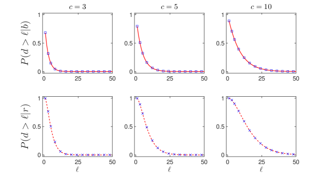
Figure 8: The conditional tail distributions $P(d>\ell|b)$ and $P(d>\ell|r)$ of first hitting times vs. $\ell$ for RWs on an ER network, for paths terminated by backtracking (top row) or by retracing (bottom row), respectively. The results are shown for $N=1000$ and $c=3$, $5$ and $10$. The theoretical results for $P(d>\ell|b)$ are obtained from Eq. (46), while the theoretical results for $P(d>\ell|r)$ are obtained from Eq. (47). In both cases, the theoretical results (solid lines) are found to be in excellent agreement with the numerical simulations (symbols).

In Fig. 8 we present the probabilities $P(d>\ell|b)$ and $P(d>\ell|r)$ that a RW will have a path of length larger than $\ell$ given that it terminates due to backtracking or retracing, respectively. The results are presented for $N=1000$ and $c=3$, $5$ and $10$. The analytical results (solid lines) are found to be in excellent agreement with the numerical simulations (circles). In both cases, the paths tend to become longer as $c$ is increasd. However, for each value of $c$, the paths which terminate by retracing are typically longer than the paths which terminate by backtracking.

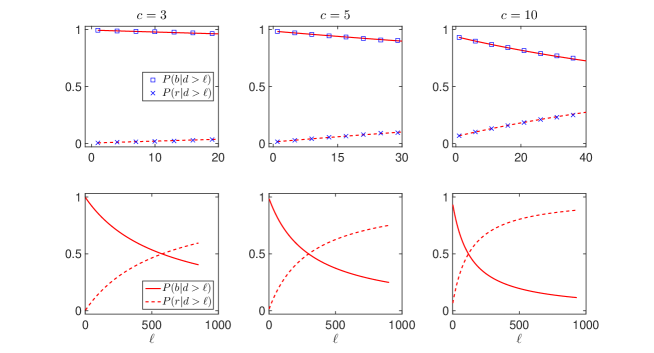
Figure 9: The conditional probabilities $P(b|d>\ell)$ and $P(r|d>\ell)$ that a RW path will terminate by backtracking or by retracing, respectively, given that its length is larger than $\ell$, are presented as a function of $\ell$. Results are shown for an ER networks of size $N=1000$ and $c=3$, $5$ and $10$. The theoretical results for $P(b|d>\ell)$ (solid lines) are obtained from Eq. (52) while the theoretical results for $P(r|d>\ell)$ (dashed lines) are obtained from Eq. (53). In the top row these results are compared to the results of numerical simulations (symbols) finding excellent agreement. This comparison is done for the range of path lengths which actually appear in the numerical simulations and for which good statistics can be obtained. Longer RW paths which extend beyond this range become extremely rare, so it is difficult to obtain sufficient numerical data. However, in the bottom row we show the theoretical results for the entire range of path lengths. It is found that $P(b|d>\ell)$ is a monotonically decreasing function of $\ell$ while $P(r|d>\ell)$ is monotonically increasing. The two curves intersect each other at a value $\ell$ where both probabilities are equal to $1/2$.

In Fig. 9 we present the probabilities $P(b|d>\ell)$ and $P(r|d>\ell)$ that a RW will terminate due to backtracking or retracing, respectively. Results are shown for ER networks of size $N=1000$ and $c=3$, $5$ and $10$. The theoretical results for $P(b|d>\ell)$ (solid lines) are obtained from Eq. (50) while the theoretical results for $P(r|d>\ell)$ (dashed lines) are obtained from Eq. (53). As expected, it is found that $P(b|d>\ell)$ is a monotonically decreasing function of $\ell$ while $P(r|d>\ell)$ is monotonically increasing. In the top row these results are compared to the results of numerical simulations (symbols) finding excellent agreement. This comparison is done for the range of path lengths which actually appear in the numerical simulations. Longer RW paths which extend beyond this range become extremely rare, so it is difficult to obtain sufficient numerical data. However, in the bottom row we show the theoretical results for the entire range of path lengths. In fact, such long paths can be sampled using the pruned enriched Rosenbluth method, which was successfully used in the context of SAWs in polymer physics [56]. In this method one samples long non-overlapping paths, keeping track of their weights, to obtain an unbiased sampling in the ensemble of all paths.

8 Summary and Discussion

We have presented analytical results for the distribution of first hitting times of random walkers on ER networks. Starting from a random initial node, these walkers hop randomly between adjacent nodes until they hit a node which they already visited before. At this point, the path is terminated. The number of steps taken from the initial node up to the termination of the path is called the first hitting time. Using recursion equations, we obtained analytical results for the distribution of first hitting times, $P(d=\ell)$. One can distinguish between two termination scenarios, referred to as backtracking and retracing. We have performed a detailed analysis of the probabilities, $p_{b}$ and $p_{r}$, that the termination will take place via the backtracking or via the retracing mechanism, respectively. We obtained analytical expressions for these probabilities in terms of the network size, $N$ and the mean degree, $c$. We also obtained analytical expressions for the conditional distributions of the path lengths, $P(d=\ell|b)$ and $P(d=\ell|r)$ for the paths which terminate by backtracking and by retracing, respectively. Finally, we obtained analytical expressions for the conditional probabilities $P(b|d=\ell)$ and $P(r|d=\ell)$ that a path which terminates after $\ell$ steps is terminated by backtracking or by retracing, respectively. It was found that the two termination mechanisms exhibit very different behavior. The backtracking probability sets in starting from the second step and is constant throughout the path. As a result, this mechanism alone whould produce a geometric distribution of path lengths. The retracing mechanisms sets in starting from the third step and its rate increases linearly in time. The balance between the two termination mechanisms depends on the mean degree of the network. In the limit of sparse networks, the backtracking mechanism is dominant and most paths are terminated long before the retracing mechanism becomes relevant. In the case of dense networks, the backtracking probability is low and most paths are terminated by the retracing mechanism.

In Table 1 we summarize the main results of the paper, providing links to the corresponding equations, for three different levels of precision. The results which are given by closed form expressions appear in boldface fonts. The first column includes exact results. Most of these results are expressed in terms of sums and products of the conditional probabilities, with no closed form expression. The second column includes the results obtained by replacing the sums by integrals. These results are of high accuracy since the relative errors invloved in the replacement of the sums by integrals are small and scale like $\ell/N$. The third column includes approximate results, which are given by closed form expressions. These results are obtained from a series expansion truncated above the second order in $\ell/N$, and the errors involved in this approximation scale like $\ell^{3}/N^{2}$. The conditional probabilities of the two termination scenarios are expressed in terms of $P(d>\ell)$ and $\ell_{\rm mean}$. Therefore, the level of precision of these conditional probabilities depends on the precision used for these input functions, as indicated by the superscripts.

Under conditions in which backtracking and retracing steps are not allowed the RW becomes an SAW. It is terminated via the stalemate scenario, when all the nodes surrounding the current node have already been visited. The resulting path length is referred to as the last hitting time. In Ref. [36] it was shown that for large networks ($N\gg 1$) the tail distribution of the last hitting times denoted by $P_{\rm L}(d>\ell)$, follows a Gompertz distribution [42, 43, 44] of the form

$$P_{\rm L}\left(d>\ell\right)\simeq\exp\left[-\frac{N}{c}e^{-c}\left(e^{\frac{c}{N}\ell}-1\right)\right],$$ (54)

and the corresponding probability density is given by

$$P_{\rm L}(d=\ell)\simeq\exp\left[-\frac{N}{c}e^{-c}\left(e^{\frac{c}{N}\ell}-1\right)-\left(1-\frac{\ell+1}{N}\right)c\right].$$ (55)

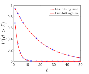
Figure 10: Theoretical results for the tail distribution $P(d>\ell)$ of the first hitting times of the RW model (solid line) and the tail distribution $P_{\rm L}(d>\ell)$ of the last hitting times of the SAW model (dashed line), on ER networks of size $N=1000$ and $c=3$. Both results are in excellent agreement with numerical simulations (symbols). As expected, the last hitting times are much longer than the first hitting times.

In Fig. 10 we present the tail distribution $P(d>\ell)$ of first hitting times (solid line) and the tail distribution $P_{\rm L}(d>\ell)$ of last hitting times (solid line) for an ER network of size $N=1000$ and mean degree of $c=3$. As expected, there is a large gap between the first hitting time and the last hitting time. This gap increases as the network becomes denser.

Beyond the specific problem of first hitting times of RW on networks, the analysis presented here provides useful insight into the general context of the distribution of life expectancies of humans, animals and machines [51, 52]. It illustrates the combination of two lethal hazards, where one hits at a fixed, age-independent rate, while the other increases linearly with age. The first hazard may be considered as an external cause such as an accident while the second hazard involves some aging related degradation which results in an increasing failure rate.

References

Table 1: Summary of the main results and their level of precision

Property	Exact	Accurate	Approximate
$p_{t}(k)$	Eq. (3)∗	–	–
$c(t)$	Eq. (4)	–	–
$P_{b}(d>\ell)$	Eq. (17)	–	–
$P_{r}(d>\ell)$	Eq. (19)	Eq. (5)	Eq. (24)
$P(d>\ell)$	Eq. (14)1	Eq. (14)2	Eq. (25)
$\ell_{\rm mean}$	Eq. (27)	Eq. (28)2	Eq. (30)
$\langle\ell^{2}\rangle$	–	–	Eq. (35)
$\sigma_{\ell}^{2}(c)$	–	–	Eq. (36)
$p_{b}$	Eq. (42)a	Eq. (42)b	Eq. (42)c
$p_{r}$	Eq. (43)a	Eq. (43)b	Eq. (43)c
$P(d>\ell|b)$	Eq. (46)1,a	Eq. (46)2,b	Eq. (46)3,c
$P(d>\ell|r)$	Eq. (47)1,a	Eq. (47)2,b	Eq. (47)3,c
$P(b|d>\ell)$	Eq. (52)1	Eq. (52)2	Eq. (52)3
$P(r|d>\ell)$	Eq. (53)1	Eq. (53)2	Eq. (53)3

^∗boldface fonts: closed-form expressions;
¹where $P_{r}(d>\ell)$ is given by Eq. (19);
²where $P_{r}(d>\ell)$ is given by Eq. (5);
³where $P_{r}(d>\ell)$ is given by Eq. (24);
^awhere $\ell_{\rm mean}$ by Eq. (27);
^bwhere $\ell_{\rm mean}$ by Eq. (28);
^cwhere $\ell_{\rm mean}$ by Eq. (30);

References

- [1] Spitzer F 1964 Principles of Random Walk (New York: Springer-Verlag)
- [2] Weiss G H 1994 Aspects and Applications of the Random Walk (New York: North Holland)
- [3] Berg H C 1993 Random Walks in Biology (Princeton: Princeton University Press)
- [4] Ibe O C 2013 Elements of Random Walk and Diffusion Processes (New Jersey: Wiley & Sons)
- [5] Fisher M E 1966 J. Chem. Phys. 44 616
- [6] De Gennes P G 1979 Scaling Concepts in Polymer Physics (Ithaca: Cornell University Press).
- [7] Evans M R and Majumdar S N 2011 Phys. Rev. Lett. 106 160601
- [8] Lopez Millán V M, Cholvi V, Lopez L and Anta A F 2012 Networks 60 71
- [9] Lawler G F 2010 Random Walk and the Heat Equation (Providence: American Mathematical Society)
- [10] Lawler G F and Limic V 2010 Random Walk: A Modern Introduction (Cambridge: Cambridge University Press)
- [11] ben-Avraham D and Havlin S 2000 Diffusion and Reactions in Fractals and Disordered Systems (Cambridge: Cambridge University Press)
- [12] Noh D J and Rieger H 2004 Phys. Rev. Lett. 92 118701
- [13] Havlin S and Cohen R 2010 Complex Networks: Structure, Robustness and Function (Cambridge University Press, New York).
- [14] Newman M E J 2010 Networks: an Introduction (Oxford: Oxford University Press).
- [15] Costa L F and Travieso G 2005 Phys. Rev. E 75 016102
- [16] Pastor-Satorras R and Vespignani A 2001 Phys. Rev. Lett. 86 3200
- [17] Barrat A, Barthélemy M and Vespignani A 2012 Dynamical Processes on Complex Networks (Boston: Cambridge University Press)
- [18] De Bacco C, Majumdar S N and Sollich P 2015 J. Phys. A 48 205004
- [19] Montroll E W and Weiss G H 1965 J. Math. Phys. 6 167
- [20] Kahn J D, Linial N, Nisan N and Saks M E 1989 J. Theor. Probab. 2 121
- [21] Redner S 2001 A Guide to First Passage Processes (Cambridge: Cambridge University Press)
- [22] Sood V, Redner S and ben-Avraham D 2005 J. Phys. A 38 109
- [23] Madras N and Slade G 1996 The Self Avoiding Walk (Boston: Birkhäuser)
- [24] Fisher M E and Sykes M F 1959 Phys. Rev. 114 45
- [25] Kesten H 1963 J. Math. Phys. 4 960
- [26] Kesten H 1964 J. Math. Phys. 5 1128
- [27] Hara T, Slade G and Sokal A D 1993 J. Stat. Phys. 72 479
- [28] Clisby N, Liang R and Slade G 2007 J. Phys. A 40 10973
- [29] Viana M P, Batista J L B, and Costa L da F 2012 Phys. Rev. E 85 036105
- [30] Clisby N 2013 J. Phys. A 46 245001
- [31] Bollobas B 2001 Random Graphs, Second Edition (London: Academic Press)
- [32] Katzav E, Nitzan M, ben-Avraham D, Krapivsky P L, Kühn R, Ross N and Biham O 2015 EPL 111 26006
- [33] Nitzan M, Katzav E, Kühn R and Biham O 2016, Phys. Rev. E, accepted for publication; arXiv:1603.04473
- [34] Karger D, Motwani R and Ramkumar G D S 1997 Algorithmica 18 82
- [35] Herrero C P 2005 Phys. Rev. E 71 016103
- [36] Tishby I, Biham O and Katzav E 2016 J. Phys. A, accepted for publication; arXiv:1603.06613
- [37] Erdős P and Rényi 1959 Publ. Math. 6 290
- [38] Erdős P and Rényi 1960 Publ. Math. Inst. Hung. Acad. Sci. 5 17
- [39] Erdős P and Rényi 1961 Bull. Inst. Int. Stat. 38 343
- [40] Herrero C P 2007 Eur. Phys. J. B. 56 71
- [41] Slade G 2011 Surveys in Stochastic Processes, Proceedings of the 33rd SPA Conference in Berlin, 2009, EMS Series of Congress Reports, eds. Blath J, Imkeller P, and Roelly S
- [42] Gompertz B 1825 Philosophical Trans. R. Soc. London A 115 513
- [43] Johnson N L, Kotz S and Balakrishnan N 1995 Continuous Univariate Distributions (New York: John Wiley & Sons)
- [44] Shklovskii B I 2005 Theory in Biosciences 123 431
- [45] Ohishi K, Okamura H and Dohi T 2009 Journal of Systems and Software 82 535
- [46] Herrero C P and Saboyá M 2003 Phys. Rev. E 68 026106
- [47] Herrero C P 2005 J. Phys. A 38 4349
- [48] Chupeau M, Bénichou O and Redner S 2016 Phys. Rev. E 93 032403
- [49] Bénichou O and Redner S 2014 Phys. Rev. Lett 113 238101
- [50] Chupeau M, Bénichou O and Redner S 2016 arXiv:1511.01347
- [51] Finkelstein M 2008 Failure Rate Modelling for Reliability and Risk (Springer-Verlag, London)
- [52] Gavrilov L A and Gavrilova N S 2001 J. theor. Biol 213 527
- [53] Papoulis A, Pillai S and Unnikrishna S 2002 Probability, Random Variables and Stochastic Processes (McGraw-Hill, Boston).
- [54] Bloom D M 1973 Amer. Math. Monthly 80 1141
- [55] Pitman J 1993 Probability (New York: Springer-Verlag)
- [56] Grassberger P 1997 Phys. Rev. E 56 3682