Permanence and Community Structure in Complex Networks
Accepted in ACM TKDD

Abstract

The goal of community detection algorithms is to identify densely-connected units within large networks. An implicit assumption is that all the constituent nodes belong equally to their associated community. However, some nodes are more important in the community than others. To date, efforts have been primarily driven to identify communities as a whole, rather than understanding to what extent an individual node belongs to its community. Therefore, most metrics for evaluating communities, for example modularity, are global. These metrics produce a score for each community, not for each individual node. In this paper, we argue that the belongingness of nodes in a community is not uniform. We quantify the degree of belongingness of a vertex within a community by a new vertex-based metric called permanence.

The central idea of permanence is based on the observation that the strength of membership of a vertex to a community depends upon two factors: (i) the the extent of connections of the vertex within its community versus outside its community, and (ii) how tightly the vertex is connected internally. We present the formulation of permanence based on these two quantities. We demonstrate that compared to other existing metrics (such as modularity, conductance and cut-ratio), the change in permanence is more commensurate to the level of perturbation in ground-truth communities. We discuss how permanence can help us understand and utilize the structure and evolution of communities by demonstrating that it can be used to – (i) measure the persistence of a vertex in a community, (ii) design strategies to strengthen the community structure, (iii) explore the core-periphery structure within a community, and (iv) select suitable initiators for message spreading.

We further show that permanence is an excellent metric for identifying communities. We demonstrate that the process of maximizing permanence (abbreviated as MaxPerm) produces meaningful communities that concur with the ground-truth community structure of the networks more accurately than eight other popular community detection algorithms. Finally, we provide mathematical proofs to demonstrate the correctness of finding communities by maximizing permanence. In particular, we show that the communities obtained by this method are (i) less affected by the changes in vertex-ordering, and (ii) more resilient to resolution limit, degeneracy of solutions and asymptotic growth of values.

1 Introduction

Community detection is the process of finding closely related groups of entities in a network. Complex networks, such as those arising in biology, social sciences and epidemiology, represent systems of interacting entities. The entities are represented as vertices in the network and their pair-wise interactions are represented as edges. A community, then, is a group of vertices that have more internal connections (i.e., connections to vertices within the group) than external connections (i.e., connections to vertices outside the group).

Most community detection algorithms are based on combinatorial optimization. The goal is to find the community assignment that leads to the optimal value of a specified network parameter, such as modularity [Newman and Girvan (2004)] or conductance [Leskovec et al. (2009)]. However, since many real-world communities are based on subjective measurements (as opposed to a formal mathematical definition), the validation of the results is done by comparing the obtained communities with known “ground-truth” communities. Very rarely do the obtained communities exactly match with ground-truth communities. Moreover, due to the phenomenon of resolution limit and degeneracy of solutions [Fortunato and Barthelemy (2007)], the optimum parameter value sometimes produces intuitively incorrect solutions. As a result, community detection is an active area of research with new optimization metrics being regularly proposed [He et al. (2013), Yang and Leskovec (2012)], that either produce more accurate results on a certain subclass of networks and/or can address some of the above discussed issues.

Almost all community detection metrics and related algorithms contain the implicit notion that all the vertices in a community belong equally to the community, i.e., the community membership is homogeneous. Therefore, the optimal score of the metric can only be obtained over the network as a whole. The information about how placement of vertices affects the community structure is lost using these current measurements. In order to include this important information, we have introduced a vertex-centric metric called permanence [Chakraborty et al. (2014)].

The key idea in formulating permanence is as follows. Most optimization metrics are based on the total internal and external connections of the vertex. We posit that the distribution of the external connections of a vertex is equally important. In particular, our vertex assignment decisions are based not on the total number of external connections but on the maximum number of external connections to any single neighboring community. If vertex $v$ is in community $S$ and vertex $u$ is in community $T$ and there exists an edge $(v,u)$, then $S$ and $T$ are neighboring communities of each other.

To the best of our knowledge, we are the first to make this distinction between the total external connections and their distribution. Permanence of a vertex thus quantifies its propensity to remain in its assigned community and the extent to which it is “pulled” [Chakraborty et al. (2014)] by the neighboring communities.

Permanence provides a heterogeneous vertex-centric measure (in the range 1 to -1) of the extent to which a vertex belongs to its community. A value of 1 indicates that a vertex is placed correctly in its community, and a value of -1 indicates the vertex does not belong to its assigned community. The permanence of the network is given by the average permanence of all the vertices of a network. It is easy to see that the more correctly the vertices are placed in their communities, the higher the overall permanence. Using this concept we propose a new community detection algorithm, MaxPerm based on optimizing the permanence of the network [Chakraborty et al. (2014)].

In this paper, after providing background information on the related work in community detection (Section 2) and the datasets that we used in our experiments (Section 3), we explain the rationale behind creating the permanence metric (Section 4). We show how change in permanence is more commensurate to perturbation of ground-truth communities as compared to other competing metrics (Section 6) and present a community detection, MaxPerm, based on maximizing permanence (Section 8) . We extend this earlier work with the following new contributions:

• In-depth Study of Network Parameters Affecting the Value of Permanence. We study how the distribution of different network parameters, such as connectivity and clustering coefficient affect the value of permanence (Sections 5 and 6).

• Use of Permanence to Understand the Structure of the Network. We show that permanence can provide a better understanding of the structure of the network, such as how to strengthen the communities and revealing the core-periphery based on the community structure, as well as its use in applications such as vertex persistence in communities of evolving networks and identifying effective initiators for message spreading (Section 7).

• In-depth Analysis of Communities Obtained using MaxPerm. The communities obtained by MaxPerm are in general of a smaller size than those obtained by other community detection methods. We study the structure of the communities obtained and show that these communities are actually well defined sub-communities (Section 8).

• Algorithmic Factors Affecting Results of MaxPerm. We study how different algorithmic factors such as ordering of the vertices and selection of initial seed communities affects the results of MaxPerm (Sections 9 and 10).

• Analytical Proof on Correctness. We provide analytical results to demonstrate how finding communities by maximizing permanence reduces the existing limitations of community detection algorithms such as resolution limit, degeneracy of solutions and asymptotic growth of values. (Section 11).

We make our experimental codes available in the spirit of reproducible research: http://cnerg.org/permanence.

2 Related Work

We present the ongoing research on two aspects of community detection: (i) algorithms to detect community and (ii) metrics for evaluating the correctness of the obtained community.

2.1 Community detection algorithms

Most of the research in community detection algorithms are based on the idea that a community is a set of nodes that has more and/or better links between its members than with the remainder of the network. Work in this area encompasses many different approaches including, modularity optimization [Blondel et al. (2008), Clauset et al. (2004), Guimera and Amaral (2005), Newman (2004b), Newman (2006)], spectral graph-partitioning algorithm [Newman (2013), Richardson et al. (2009)], clique percolation [Farkas et al. (2007), Palla et al. (2005)], local expansion [Baumes et al. (2005), Lancichinetti et al. (2009)], fuzzy clustering [Psorakis et al. (2011), Sun et al. (2011)], link partitioning [Ahn et al. (2010), Evans and Lambiotte (2009)], random-walk based approach [De Meo et al. (2013a), Pons and Latapy (2006)], information theoretic approach [Rosvall and Bergstrom (2007), Rosvall and Bergstrom (2008)], diffusion-based approach [Raghavan et al. (2007a)], significance-based approach [Lancichinetti et al. (2010)] and label propagation [Raghavan et al. (2007b), Xie and Szymanski (2011), Xie and Szymanski (2012)].

However most of these algorithms produce different community assignments if certain algorithmic factors, such as the order in which the vertices are processed, changes. [Lancichinetti and Fortunato (2012a)] proposed consensus clustering by re-weighting the edges based on how many times the pair of vertices were allocated to the same community, for different identification methods. Several pre-processing techniques [Bader et al. (2013), Riedy et al. (2011)] have been developed to improve the quality of the solution. These methods form an initial estimate of the community allocation over a small percentage of the vertices and then refine this estimate over successive steps. Recently, [Chakraborty et al. (2013)] pointed out how vertex ordering influences the results of the community detection algorithms. They identified invariant groups of vertices (named as “constant communities”) whose assignment to communities are not affected by vertex ordering.

2.2 Community evaluation metrics

Most community detection algorithms are based on optimizing a combinatorial metric. Examples of such metrics include conductance [Leskovec et al. (2009), Kannan et al. (2000), Shi and Malik (2000)], cut-ratio [Fortunato (2010), Leskovec et al. (2010)]; however, the most popular and widely accepted metric is modularity [Newman (2006), Newman and Girvan (2004)]. It is defined as the difference (relative to the total number of edges) between the actual and the expected (in a randomized graph with the same number of nodes and the same degree sequence) number of edges inside a given community. Although initially defined for undirected and unweighted networks, the definition of modularity has been extended to capture community structure in weighted [Newman (2004a)] and directed [Leicht and Newman (2008)] networks.

It was also demonstrated that modularity suffers from a resolution limit, that is, by optimizing modularity we cannot find communities smaller than a threshold size [Fortunato and Barthelemy (2007)], or weight [Berry et al. (2011)]. The threshold depends on the total number (or total weight) of edges in the network and on the degree of interconnectedness between communities. Later, [Good et al. (2010)] also showed that optimizing modularity can lead to degeneracy of solutions, i.e., an exponential number of high (and nearly equal)-modularity but structurally distinct solutions from a single graph. They also studied the (asymptotic) growth of modularity, showing that it depends strongly both on the size of the network and the number of modules it contains.

To address the resolution limit problem, multi-resolution versions of modularity [Arenas et al. (2008), Reichardt and Bornholdt (2006)] were proposed to allow researchers to specify a tunable target resolution limit parameter. [Lambiotte (2010)] proposed different types of multi-resolution quality functions to tackle resolution limit problem. [He et al. (2013)] considered different community densities as good quality measures for community identification, which do not suffer from resolution limits. Furthermore, [Lancichinetti and Fortunato (2011)] stated that even those multi-resolution versions of modularity are inclined to merge the smallest well-formed communities, and to split the largest well-formed communities. Recently, [Chen et al. (2013)] proposed Modularity Density metric to solve the problems raised by [Lancichinetti and Fortunato (2011)]. A detailed review can be found in [Chakraborty et al. (2016a)].

Metrics to compare with ground-truth communities: Although all these metrics mentioned above are useful in analytically evaluating a community structure, a stronger measure of correctness is to compare the obtained community structure with the actual known community structure (ground-truth) of a network. To compare these two community structures, different validation metrics have been proposed, such as Normalized Mutual Information (NMI) [Danon et al. (2005)], Adjusted Rand Index (ARI) [Hubert and Arabie (1985)] and Purity (PU) [Manning et al. (2008)]. However, [Orman et al. (2012)] argued that these metrics are not completely relevant in the context of network analysis, because they ignore the network structure. They proposed the weighted versions of these measures where misplacing a high degree vertex would incur higher penalty compared to a low degree vertex. In our experiments, we, therefore, also use the weighted versions of these measures, namely Weighted-NMI (W-NMI), Weighted-ARI (W-ARI) and Weighted-Purity (W-PU) (we refer the reader to the paper [Orman et al. (2012)] for the detailed descriptions of these metrics). Note that all the metrics are bounded between 0 (no matching) and 1 (perfect matching).

3 Network Datasets and Ground-truth Communities

We examine a set of artificially generated networks and three real-world complex networks whose underlying ground-truth community structures are known to us. The brief description of the used datasets and their ground-truth communities are mentioned below.

3.1 Synthetic networks

We select the LFR benchmark model [Lancichinetti and Fortunato (2009)] to generate artificial networks with a community structure. The model allows to control directly the following properties: number of nodes $n$, desired average degree $k$ and maximal degree $k_{max}$, exponent $\gamma$ for the degree distribution, exponent $\beta$ for the community size distribution, and mixing coefficient $\mu$. The parameter $\mu$ represents the desired average proportion of links between a node and the nodes located outside its community, called inter-community links. Unless otherwise stated, the LFR network is generated with the number of nodes ($n$) as 1000, and $\mu$ is varied from 0.1 to 0.6. For the rest of the parameters, we use the default value of the parameters mentioned in the implementation designed by [Lancichinetti and Fortunato (2009)].

Properties of real-world networks. $n$ and $e$ are the number of nodes and edges, $c$ is the number of communities, $<k>$ and $k_{max}$ its average and maximum degree, $n_{c}^{min}$ and $n_{c}^{max}$ the sizes of its smallest and largest communities. Network $n$ $e$ $<k>$ $k_{max}$ $c$ $n_{c}^{max}$ $n_{c}^{min}$ Football 115 613 10.57 12 12 13 5 Railway 301 1,224 6.36 48 21 46 1 Coauthorship 103,677 352,183 5.53 1,230 24 14,404 34

3.2 Real-world networks

We use three real-world networks mentioned below whose ground-truth community structures are known a priori. The properties of these dataset are summarized in Table 3.1.

Football network [Girvan and Newman (2002)] contains the network of American football games between Division IA colleges during the regular season of Fall 2000. The vertices in the graph represent teams (identified by their college names) and edges represent regular-season games between the two teams they connect. The teams are divided into conferences (indicating communities) containing around 8-12 teams each.

Railway network [Ghosh et al. (2011)] consists of nodes representing stations, where two stations $s_{i}$ and $s_{j}$ are connected by an edge if there exists at least one train-route such that both $s_{i}$ and $s_{j}$ are scheduled halts on that route. Here the communities are states/provinces of India since the number of trains within each state is much higher than the trains in-between two states.

Coauthorship network [Chakrabort et al. (2013)] is derived from the citation dataset. Here each node represents an author and an undirected edge between authors is drawn if the two authors collaborate at least once via publishing a paper. The communities are marked by the research fields since authors have a tendency to collaborate with other authors within the same field. Besides the aggregated network, we also create some intermediate networks mentioned in Table 6 by cumulatively aggregating all the vertices and edges over each year, e.g., 1960-1971, 1960-1972, …, 1960-1980.

Figure 1: (Color online) Toy example depicting permanence of two vertices $u$ and $v$. The communities are represented by broken lines.

4 Defining Permanence

In this section, we describe the permanence metric and the two primary concepts behind its formulation.

Concept I: A vertex should have more number of internal connections than the number of connections to any of the external neighboring communities.

Most optimization metrics consider the total number of external neighbors of the vertex. However, in our earlier experiment [Chakraborty et al. (2014), Chakraborty (2015), Chakraborty et al. (2016b)], we empirically demonstrated that a group of vertices are likely to be placed together so long as the number of internal connections is larger than the number of connections to any one single external community. In other words, a vertex which has connections to some external communities, experiences a separate “pull” from each of these external communities. In formulating permanence we consider the maximum pull, which is proportional to the maximum number of connections to an external community (see Figure 1).

Concept II: Within the substructure of a community, the internal neighbors of the vertex should be highly connected among each other.

Most optimization metrics only consider the internal connections of a vertex within its own community. However, how strongly a vertex is connected also depends on whether its internal neighbors are connected with each other. To measure this connectedness of a vertex, we compute the clustering coefficient of the vertex with respect to its internal neighbors. For a vertex $v$ belonging to community $c$, it is measured by the ratio between the actual number of edges among the neighbors (which also belong to $c$) of $v$ and the total number of possible edges among the neighbors [Holland and Leinhardt (1971)]. The higher this internal clustering coefficient, the more tightly the vertex is connected to its community (see Figure 1).

We combine these two criteria to formulate permanence of a vertex $v$, as follows:

$$Perm(v)=\Big{[}\frac{I(v)}{E_{max}(v)}\times\frac{1}{D(v)}\Big{]}-\Big{[}1-c_{in}(v)\Big{]}$$ (1)

where $I(v)$ is the number of internal (in its own community) neighbors of $v$, $E_{max}(v)$ is the maximum number of connections of $v$ to any one of the external communities, $D(v)$ is the degree of $v$ and $c_{in}(v)$ is the clustering coefficient among the internal neighbors of $v$. Figure 1 presents a toy example to calculate the permanence of a vertex.

For vertices that do not have any external connections, $Perm(v)$ is considered to be equal to the internal clustering coefficient (i.e., $Perm(v)=c_{in}(v)$). If the number of internal connections, $I(v)$, is less than 2, we set the internal clustering coefficient, $c_{in}(v)$, to be 0. Therefore, for a vertex in a singleton community, $Perm(v)=0$.

The maximum value of $Perm(v)$ is 1 and is obtained when vertex $v$ is an internal node and part of a clique. The lower bound of $Perm(v)$ is close to -1. This is obtained when $I(v)\ll D(v)$, such that $\frac{I(v)}{D(v)E_{max}(v)}\approx 0$ and $c_{in}(v)=0$. Therefore for every vertex $v$, $-1<Perm(v)\leq 1$. The permanence of a graph $G(V,E)$, where $V$ is the set of vertices and $E$ is the set of edges, is given by $Perm(G)=\frac{1}{|V|}\sum_{v\in V}Perm(v)$. For a graph $G(V,E)$, the range is $-1<Perm(G)\leq 1$. $Perm(G)$ will be closer to 1 if majority of vertices have high permanence, that is the vertices are in well-defined communities. This can happen only if the network inherently possesses a strong community structure.

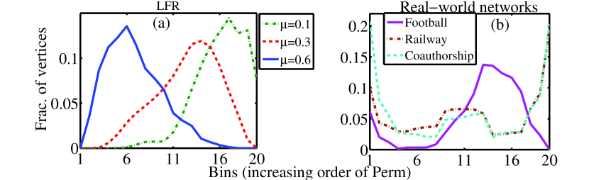
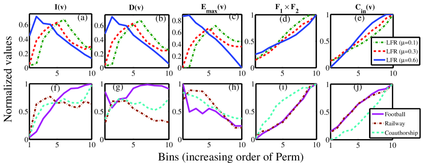
Figure 2: (Color online) Distribution of the values of Perm for different networks. The value of Perm of vertices is equally divided into 20 buckets indicated in x-axis (bin 1: $-1\leq Perm<-0.9$, …, bin 20: $0.9\leq Perm\leq 1$).

Figure 3: (Color online) The relation of average Perm with (a),(f) $<I(v)>$, average internal neighbors per vertex, (b),(g) $<D(v)>$, average degree per vertex, (c),(h) $<E_{max}(v)>$, average maximum connections to an external community per vertex, (d),(i) average value of $F_{1}\times F_{2}=\frac{I(v)}{D(v)}\times\frac{1}{E_{max}(v)}$ per vertex, (e),(j) $<C_{in}(v)>$, average internal clustering coefficient per vertex for LFR (upper panel) and real-world (lower panel) networks.

5 Effect of individual components on permanence

In this section, we study the distribution of permanence values corresponding to the vertices in the graph based on their communities. We first compute the permanence of each vertex based on the ground-truth communities of the benchmark networks. We divide the permanence values ranging from $-1$ to $1$ into 20 bins where the low (high) numbered bins contain nodes with lower (higher) permanence. We plot the bins on x-axis, and for each bin, on the y-axis, we plot the fraction of vertices whose permanence value falls in that bin. We observe in Figures 3(a) that this curve follows a Gaussian-like distribution, i.e., there are few vertices with very high or very low permanence values with a peak at the intermediate values. The peak shifts from left to right with the decrease of $\mu$ value in the LFR network (keeping the other parameters of LFR constant). The shift in the peak shows that as the communities get more well-defined with the decrease of $\mu$, most vertices move towards higher permanence. Figure 3(b) shows that Football network also follows similar kind of behavior, where most of the vertices fall in medium Perm range. However, for Railway and Coauthorship networks, the curve follows “U-shaped” pattern, indicating maximum vertices falling in either very low or very high permanence buckets.

This phenomenon indicates that the community structure is not very clear in these networks. Recall that we have computed communities from ground-truths. The high proportion of lower values indicates that the networks contain entities that are not easy to classify, such as railway stations that are at the border of the states or authors who publish in multiple fields.

To understand the dependence on each component of the permanence equation (Equation 1), we further plot permanence with respect to each individual component, i.e., $I(v)$, $D(v)$, $E_{max}(v)$, $C_{in}(v)$ and their combination in Figure 3. Figure 3(a) shows a decreasing trend of $I(v)$ with the increase of permanence for LFR, where the pattern is completely opposite for real-world networks as shown in Figure 3(f). The trend is almost similar for the relation between $D(v)$ and permanence in Figures 3(b) and 3(g). However, here most of the real-world networks except Football show similar pattern with that of LFR, where high degree nodes tend to exhibit low or medium permanence value. Further, we plot the relation between permanence and $E_{max}(v)$ in Figures 3(c) and 3(h) and observe that while all the real-world networks show an inverse relation, for two LFR networks ($\mu=0.3$ and $\mu=0.6$) it initially increases and then starts decreasing. From these observations, one can not find any universal relation as such among different networks. However, once we combine these factors together and plot the dependence between permanence and $\frac{I(v)}{D(v)}\times\frac{1}{E_{max}(v)}$ in Figures 3(d) and 3(i), we observe a consistent behavior for all the networks in that the value of the combination tends to increase almost linearly with permanence. A similar trend is followed in Figures 3(e) and 3(j) where the value of internal clustering coefficient tends to increase with the increase of permanence. These results show that permanence depends on two factors – (i) the combined effect of $\frac{I(v)}{D(v)}\times\frac{1}{E_{max}(v)}$, and (ii) the value of $C_{in}(v)$.

6 Effect of perturbations on ground-truth communities

One of the crucial measures for an effective community scoring metric is how it behaves under different perturbations of the ground-truth community structure [Yang and Leskovec (2012)]. The metric should be robust to small perturbations of the ground-truth communities, such as when groupings of nodes that differ very slightly from the original ground-truth grouping. Furthermore, the metric should also be sensitive to large perturbations. If the change is so large that the ground-truth structure dissolves to a random set of nodes, then the value of the scoring function should be low. In this section, we compare the change in value of permanence with three other community scoring metrics and demonstrate that among them permanence is both robust to noise as well as sensitive to large changes in the network.

6.1 Community scoring metrics

We consider the following community scoring metrics:

• Modularity (Mod): Modularity [Newman (2006)] is defined by the fraction of the edges that fall within the given groups minus the expected such fraction if edges were distributed at random. Formally, for a given graph $G(V,E)$, it is quantified as follows:

  $$Q=\frac{1}{2m}\sum_{u,v\in V}[A_{uv}-\frac{k_{u}k_{v}}{2m}]\delta(c_{u},c_{v})$$ (2)

  where $m=|E|$, $A_{uv}$ is the $(u,v)$ entry of the adjacency matrix $A$, $k_{u}$ is the degree of vertex $u$, $c_{u}$ is the community of vertex $u$, and $\delta(c_{u},c_{v})=1$ if $u$ and $v$ are in the same community or $0$ otherwise.

• Conductance (Con): Conductance [Leskovec et al. (2009)] is the ratio between the number of edges inside the cluster and the number of edges leaving the cluster [Kannan et al. (2000), Shi and Malik (2000)]. More formally, conductance $\Phi(S)$ of a set of nodes $S$ is defined as follow:

  $$\Phi(S)=\frac{C_{S}}{min(Vol(S),Vol(V\setminus S))}$$ (3)

  where $C_{S}$ denotes the size of the edge boundary, $C_{S}=|{(u,v)}:u\in S,v\notin S|$, and $Vol(S)=\sum_{u\in S}d_{u}$ where $d_{u}$ is the degree of vertex $u$.

• Cut-ratio (Cut): Cut-ratio is a standard metric in graph clustering [Fortunato (2010), Leskovec et al. (2010)], which is defined as the fraction of all possible edges leaving the cluster $S$. Formally, given an undirected graph $G(u,v)$, the cut-ratio $\theta(S)$ of a set of nodes $S$ is defined as follow:

  $$\theta(S)=\frac{C_{S}}{n_{S}(n-n_{S})}$$ (4)

  where $C_{S}$ is defined earlier, and $n_{S}=|S|$.

Note that the higher the value of modularity, the better the quality of the community structure; however for conductance and cut-ratio, the opposite argument is applicable. Therefore, to make these two measures comparable to modularity and permanence, we measure (1-Con) and (1-Cut) for conductance and cut-ratio respectively.

6.2 Perturbation strategies

Given a graph $G=<V,E>$ and perturbation intensity $p$, we restructure the ground-truth community by applying a perturbation strategy. We experiment with the three perturbation strategies as proposed in [Yang and Leskovec (2012)]. We designate a given ground-truth community as $S$ and the rest of the network as $S^{\prime}$.

1. Edge-based perturbation: We select an inter-community edge $(u,v)$ where $u\in S$ and $v\in S^{\prime}$ (where $S\neq S^{\prime}$) and assign $u$ to $S^{\prime}$ and $v$ to $S$. We continue this process for $p\cdot|E|$ iterations. This strategy preserves the size of $S$, but certain vertices within the ground-truth community may become disconnected.

2. Random perturbation: We pick two random nodes $u\in S$ and $v\in S^{\prime}$ (where $S\neq S^{\prime}$) that may not be connected by an edge and then swap their memberships. We continue this process for $p\cdot|V|$ iterations. Random perturbation maintains the size of $S$, but the community may have disconnected vertices.

3. Community-based perturbation: This perturbation is similar to the edge-based strategy. However, each community $S$ is perturbed one by one for $p\cdot|S|$, until the nodes of the community are swapped with nodes outside the community. This process is repeated for all the communities separately.

We perturb networks using these perturbation strategies for values of $p$ ranging between 0.01 to 0.5. We compute how the perturbations, as given by the value of $p$, affect the values of modularity, permanence, 1-Con and 1-Cut. For small values of $p$, small change of the scoring function is desirable. This indicates that the scoring function is robust to noise. For high perturbation, that is larger values of $p$, the communities become more random. Therefore, the values should drop significantly.

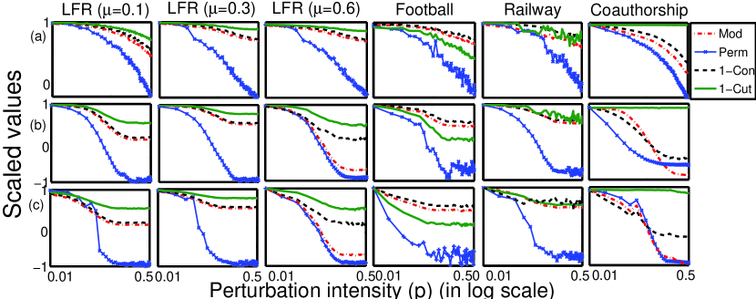
Figure 4: (Color online) Change in the value of the scoring functions with the increase of perturbation intensity $p$ in (a) edge-based, (b) random and (c) community-based perturbation strategies. The values are normalized by the maximum value obtained from each function.

6.3 Experimental results

Figure 4 shows the results of our experiments. To compare equitably across the different scoring functions, we scale the values of each parameter by normalizing with the maximum value obtained from that function. For all three strategies, the scoring function values decrease with the increase of $p$. Of the three methods Community-based produces the fastest degradation, followed by Random perturbation and Edge-based perturbation is the slowest. However, once $p$ has reached a certain threshold, the decrease is much faster in permanence, while other scoring functions do not always show this sensitivity to large perturbation.

In order to further observe how perturbation affects each of the three major components of the permanence metric, namely the internal degree $I(v)$, the maximum external connections $E_{max}(v)$ and the internal clustering-coefficient $c_{in}(v)$, we further measure the change of their individual values as a function of $p$. Figure 5 shows the rate of these changes for random perturbation. The most sensitive components of permanence are the internal degree and the average internal clustering-coefficient of vertices. These values tend to be comparatively stable for small perturbations, but degrades significantly as $p$ increases. This provides another justification for incorporating the internal clustering-coefficient as a penalty factor in the formulation of permanence.

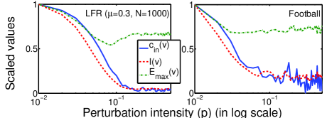
Figure 5: (Color online) Change in the average values of internal degree $I(v)$, maximum external connections $E_{max}(v)$ and internal clustering-coefficient $c_{in}(v)$ of vertices of two representative networks with the increase of perturbation intensity in random perturbation strategy.

7 Implications of permanence

We have shown in [Chakraborty et al. (2014)], using a rank correlation approach, that permanence is a better quality scoring metric as compared to modularity, conductance and cut-ratio. In Section 6, we demonstrated how permanence is robust to small perturbations and sensitive to larger ones. In this section, we analyze the characteristics of permanence from different perspectives of community structure, based on their known ground-truth structure.

7.1 Measuring persistence of a vertex in its community

We observe, using the metadata of the co-authorship networks, that the permanence of a vertex is proportional to its persistence, i.e., how long a vertex remains in an evolving community. In the original publication dataset [Chakrabort et al. (2013)] as mentioned in Section 3, each scientific article is categorized into one of the 24 research fields (such as Algorithms, Programming Languages, AI etc.). We tag each author by the field in which she has published maximum papers. Each field corresponds to a community [Chakrabort et al. (2013)]. Essentially, we intend to measure the persistence of an author in her own community in terms of her research age. For this, we define research age ($\xi$) of an author in a field/community in two different ways as follows.

Definition 1: Collective research age ($\xi_{c}$): The collective research age $\xi_{c}^{f}(a)$ of an author $a$ in a field/community $f$ is defined by the total number of distinct years author $a$ has published at least one paper in the field $f$.

Definition 2: Discounted research age ($\xi_{d}$): The discounted research age $\xi_{d}^{f}(a)$ of an author $a$ in a field/community $f$ is defined by the total number of distinct years author $a$ has published at least one paper in the field $f$, where each year is linearly penalized by the number of its immediate consecutive preceding years when she has not published a single paper on $f$. The linear penalty is introduced to bring in the effect of “consistency break” in the publication career of an author. Ideally, an author who is publishing consistently in a field should be more persistent than an author publishing in stretches with intermediate gaps. The penalty is used to significantly put more emphasis on the former case than the latter case.

For example, let us assume that an author $a$ has published papers in the following years: 1960, 1965, 1966, 1967, 1970. Therefore, $\xi_{c}^{f}(a)=5$ and $\xi_{d}^{f}(a)=(1+1/4+1+1+1/2)=3.75$ (year 1965 is penalized by its previous 4 consecutive unproductive years, similarly for 1970). We then plot the average degree and the average permanence of authors against two types of research ages in Figure 6. We observe that while there is almost no correlation between the average degree and the research age of an author, the permanence value of an author is almost linearly correlated with the research age. This evidence essentially leads to the the following conclusions: (i) permanence of a vertex is a suitable way of representing its persistence in its own community, which can not be derived from the degree of a vertex, (ii) since the result in Figure 6 is reported over all the authors in different communities, we can also compare the extent of persistence of two vertices belonging to two different communities, i.e., same permanence value of two vertices in two different communities indicates the equal extent of persistence in their corresponding communities.

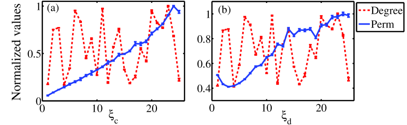
Figure 6: Changes of average degree and average permanence (with variance) of authors with the increase in (a) collective research age $\xi_{c}$, and (b) discounted research age $\xi_{d}$.

7.2 Strengthening the community structure

The value of permanence of a vertex signifies its propensity to remain in its own community. Therefore, vertices having low permanence in a community are loosely connected to the community. We explore whether we can strengthen the community structure by deleting vertices with low permanence. Note that when a vertex is deleted from its community, it would also affect the permanence value of the remaining vertices. Therefore, we rank the vertices at the very beginning based on permanence and do not consider further changes in permanence during the deletion. Then in each step, we measure the quality of the cluster by edge-density (ratio between the actual number of edges and the expected number of edges in that cluster).

For each community, we remove top $n\%$ low ranked vertices based on permanence and measure the percentage change of edge-density (averaged over all the communities) due to this removal. One can observe in Figure 7 that the edge-density increases with the increase in $n$. Although overall there is increase in edge density, we notice that in LFR ($\mu=0.6$), the edge-density starts decreasing after removing 35% of vertices. The reason might be described as follows. In LFR ($\mu=0.6$) vertices generally exhibit small permanence value due to the overall inferior community structure. The range of permanence values of vertices in each community of LFR ($\mu=0.6$) is also not high as compared to the same for LFR ($\mu=0.1$). Therefore, removing 35% of vertices from LFR ($\mu=0.6$) might result in the removal of vertices having relatively high ranking based on permanence. On the other hand, since the range is high for LFR ($\mu=0.1$) and LFR ($\mu=0.3$), the same extent of deletion of vertices might not affect the high-ranked vertices in the community. However for these networks, such decrease in edge-density can also be observed for higher extent of deletion (usually beyond 50%, not shown in Figure 7).

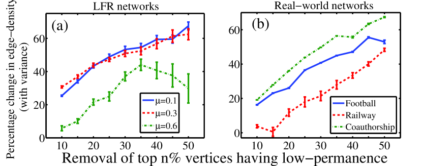
Figure 7: (Color online) Percentage change in edge-density after removing top $n\%$ (varies from 10% to 50%) low-ranked vertices based on permanence. Each point in this plot is averaged over all the communities, and therefore, the variance is also plotted.

7.3 Heterogeneity and core-periphery organization of community structure

Although it is implicitly assumed that all the constituent members of a community belong to the community equally, this is not true in reality. Within a community, the extent of involvement and activity may not be same for all members – permanence can capture this heterogeneity. The permanence of a node $v$ belonging to a community $c$ indicates the extent to which the node belongs to the community. With this value several inferences can be drawn about the communities present. For instance, it inherently creates a gradation/ranking of the constituent vertices in a community. This ranking may be important in many cases – for example in exploring the core-periphery structure of a community.

To explore the relation of permanence of a vertex with its position vis-a-vis core of a community, we use farness centrality ($d$) proposed in [Yang and Leskovec (2014)] as a measure to locate the position of a vertex within a community. In order to measure farness centrality for each community, we construct the induced subgraph constituting all the nodes in the community and measure average shortest path for each vertex within this subgraph. Thus, the lower the value of $d$ for a vertex, the closer the vertex is to the core part of the community. We plot average permanence of vertices as a function of farness centrality in Figure 8. We observe that for both LFR and real-world networks, average permanence decreases with the distance from the center of the community. Therefore, the value of permanence can act as a strong indicator of the position of the vertex in the community.

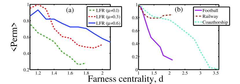
Figure 8: (Color online) Community-wise average permanence, $<Perm>$ of vertices as a function of farness centrality $d$ for LFR and real-world networks.

The next investigation reveals the manner in which the permanence value of vertices decreases from the core. A smooth decrease in value would indicate that the nodes in a community are arranged in layers with each layer of vertices roughly having similar permanence. In order to understand the mixing pattern of vertices we measure permanence-based assortativity ($r$) [Newman (2003)] to observe the preference for a network’s nodes in a community $c$ to attach to other nodes that have nearly similar permanence. We divide the permanence values into 20 bins so that nodes within a bin are considered to have equivalent permanence values, and then measure $r$ of a network. For comparison, we also measure degree-based assortativity of vertices in each network. We observe in Table 1 that both synthetic and real-world networks are highly assortative in terms of permanence, rather than in terms of degree. This result indeed indicates that in general, a community is organized into several layers, where each layer is composed of vertices exhibiting similar permanence, and vertices tend to be highly connected within each layer than across different layers.

Table 1: Average of the assortativity scores, $<r>$ (degree-based and $Perm$-based) of the communities per network.

$<r>$	LFR ($\mu=0.1$)	LFR ($\mu=0.3$)	LFR ($\mu=0.6$)
Degree-based	0.088	0.108	0.082
$Perm$ based	0.520	0.551	0.430

$<r>$	Football	Railway	Coauthorship
Degree-based	-0.105	0.153	0.155
$Perm$ based	0.747	0.531	0.489

7.4 Initiator selection for message spreading

Message spreading is one of the challenging problems in complex networks and distributed systems [Chierichetti et al. (2010)]. Starting with one source node/initiator having a message, the protocol proceeds in a sequence of synchronous rounds with the goal of delivering it to every node in the network. At every time step, each node in the system having the message communicates with one node (not having the message) in its neighborhood and transfers the message. The algorithm terminates when all the nodes in the system have received the message. A fundamental issue in message spreading is the selection of initiators. Selecting initiators based on the degree leads to faster spreading (requires less steps in average) of message than the random node selection [Demers et al. (1987)]. Since vertices with higher permanence form the core of the community, we posit that initiator selection based on permanence would help in faster dissemination of the message. Note the message spreading algorithms are based on only the local view of the vertices, therefore global methods such as those described in [Kempe et al. (2003)] will not be applicable under this formulation.

To validate this hypothesis, we consider the LFR network and vary the number of nodes from 10,000 to 90,000, keeping the other parameters constant (see Section 3). We select multiple initiators by picking one node per community present in the ground-truth structure based on the following criteria separately: (i) random, (ii) highest degree, (iii) highest permanence. For each network configuration, we run 500 simulations and report in Figure 9 the average number of time steps required for the message to reach all the nodes in the network. We observe that the permanence based initiator selection from ground-truth communities requires minimum time steps to spread the message compared to the degree-based selection.

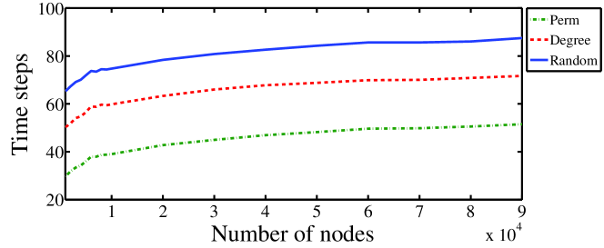
Figure 9: (Color online) Number of time steps required to broadcast a message in LFR network by varying the number of nodes.

8 Community detection using permanence maximization

We now present an algorithm for detecting communities by maximizing the permanence of the network. Our algorithm, MaxPerm (pseudocode in Algorithm 1), finds high permanence partitions of large networks using a greedy agglomerative approach, similar to the methods used in [Blondel et al. (2008), Clauset et al. (2004)].

Initially the vertices are assigned to random connected subgraphs as their initial seed community. At each iteration, a vertex is moved from one community to another if its permanence increases. This process is continued for several iterations until the value of the permanence of the network is unchanged. Although convergence to a fixed value is not theoretically guaranteed, we have observed that on test cases the algorithm converges within ten iterations. As in the case of modularity-maximization methods, we observe that creation of appropriate seed communities can help improve the quality of community detection. We shall discuss this issue later in Section 10.

Data: A graph $G(V,E)$

Result: Permanence of $G$; Detected communities

Each vertex is assigned to its seed community;

Set value of maximum iteration as $maxIt$ ;

$vertices\leftarrow|V|$;

$Sum\leftarrow 0$;

$Old\_Sum\leftarrow-1$;

$Itern\leftarrow 0$;

while $Sum\neq Old\_Sum$ and $Itern<maxIt$ do

       $Itern\leftarrow Itern+1$;

       $Old\_Sum\leftarrow Sum$;

       $Sum\leftarrow 0$;

       forall $v\in V$ do

             // Compute current permanence of $v$

             $cur\_p\leftarrow Perm(v)$;

             if $cur\_p==1$ then

                   $Sum\leftarrow Sum+cur\_p$;

                   continue;;

                  

             end if

            $cur\_p\_neig\leftarrow 0$;

             $Neig(v)$=set of neighbors of $v$;

             forall $u\in Neig(v)$ do

                   // Compute current permanence of $u$

                   $cur\_p\_neig\leftarrow cur\_p\_neig+Perm(u)$;

                  

             end forall

            

            // $Comm(v)$ is the set of neighboring communities of $v$

             forall $C\in Comm(v)$ do

                   Move $v$ to community $C$;

                   // Compute permanence of $v$ in community $C$

                   $n\_p\leftarrow Perm(v)$ ;

                   // Neighbors of $v$ are affected for this movement

                   $n\_p\_neig\leftarrow 0$;

                   forall $u\in Neig(v)$ do

                         // Compute new permanence of $u$

                         $n\_p\_neig\leftarrow n\_p\_neig+Perm(u)$;

                        

                   end forall

                  if ($cur\_p<n\_p)$ and ($cur\_p\_neig<n\_p\_neig)$ then

                         $cur\_p\leftarrow n\_p$;

                        

                  else

                         Replace $v$ to its original community;

                        

                   end if

                  

             end forall

            $Sum\leftarrow Sum+cur\_p$;

            

       end forall

      

end while

$Netw\_perm=Sum/vertices$ ;

  // Permanence of $G$

Return $Netw\_perm$;

ALGORITHM 1 MaxPerm: Community Detection using Maximizing Permanence

8.1 Computational complexity and strategies for improvement

The computational complexity of the algorithm is as follows. The most expensive part in computing the permanence of a vertex $v$ is the internal clustering co-efficient, $c_{in}(v)$. Given the degree of vertex $v$ is $D(v)$, computing $c_{in}(v)$ takes time $O(D(v)^{2})$. For each vertex we compute the permanence for its own and each of its neighboring communities. Let the number of neighboring communities of vertex $v$ at iteration $k$ be $C_{k}(v)$. Let the total number of iterations required by the algorithm be $maxIt$. Therefore, the time to execute ${MaxPerm}$ is: $\sum_{k=1}^{k=maxIt}\sum_{v=1}^{v=|V|}(C_{k}(v)O(D(v)^{2}))$.

Let $d_{max}$ be the maximum degree of the network. We also note that the maximum number of communities that a node can belong to is $d_{max}+1$. The upper bound for ${MaxPerm}$ is $O(maxIt\cdot|V|\cdot d_{max}^{3})$. Since only a few nodes of the network has the highest degree, in practice the time is much lower than the value given by this upper bound.

The execution time can be further reduced by a few simple strategies. First, instead of recomputing $Perm(v)$, for each community, we can store the number of edges each vertex has in each of its neighboring communities. We update these values only when a vertex or its neighbor changes communities. Second, since we want the permanence to increase if a vertex changes communities, the only communities to consider for relocation are those with both high internal degree and high clustering coefficient. By computing permanence for only communities that satisfy these criteria we can reduce the computation time. Both these strategies require us to keep track of the communities for neighbors of the vertex, for each vertex. Together, this requires extra storage of order $O(|V|D(v))\approx O(E)$.

8.2 Baseline community detection algorithms

There exist numerous community detection algorithms, which differ in the way they define the community structure. Here we select the following set of algorithms and categorize them according to the principle they use to identify communities as per [Orman et al. (2012)].

1. Modularity-based approaches: We select three modularity optimization algorithms, namely FastGreedy approach [Newman (2004b)], Louvain [Blondel et al. (2008)] and CNM [Clauset et al. (2004)], which differ in the way they perform this optimization.

2. Node similarity-based approaches: This category deals with the notion that a community is viewed as a group of nodes which are similar to each other, but dissimilar from the rest of the network. It includes WalkTrap [Pons and Latapy (2006)] which is built on the notion that random walks tend to get trapped into a community.

3. Compression-based approaches: These approaches assume the community structure as a set of regularities in the network topology, which can be used to represent the whole network in a more compact way than the whole adjacency matrix. The best community structure is supposed to be the one maximizing compactness while minimizing information loss. The quality of the representation is assessed through measures derived from information theory. Two popular such algorithms are InfoMod [Rosvall and Bergstrom (2007)] and InfoMap [Rosvall and Bergstrom (2008)].

4. Significance-based approaches: According to these approaches, a community structure can be expected under certain circumstances, but groups of densely connected nodes can also appear only by chance. Order Statistics Local Optimization Method (OSLOM) [Lancichinetti et al. (2010)] is a local optimization method applied to measure the statistical significance of individual communities.

5. Diffusion-based approaches: These approaches rely on the assumption that information is more efficiently exchanged between nodes of the same community. In Community Overlap Propagation Algorithm (COPRA) [Raghavan et al. (2007b)], the information takes the form of a label, and the propagation mechanism relies on a vote between neighbors. Communities are then obtained by considering groups of nodes with the same label.

Each algorithm is used with its default parameters. Although the algorithms OSLOM and COPRA are suitable for overlapping community detection, these are used here to detect mutually exclusive communities (i.e., non-overlapping communities) by setting a priori the number of overlapping nodes as zero.

8.3 Validation measures

A stronger test of the correctness of the community detection algorithm, however, is by comparing the obtained community with a given ground-truth structure. We use three standard validation metrics, namely Normalized Mutual Information (NMI) [Danon et al. (2005)], Adjusted Rand Index (ARI) [Hubert and Arabie (1985)] and Purity (PU) [Manning et al. (2008)] to measure the accuracy of the detected communities with respect to the ground-truth community structure. [Orman et al. (2012)] argue that these metrics ignore the network structure and propose the weighted versions of these measures where misplacing a high degree vertices would incur higher penalty. We therefore also use the weighted versions of these measures, namely Weighted-NMI (W-NMI), Weighted-ARI (W-ARI) and Weighted-Purity (W-PU). All these metrics are bounded between 0 (no matching) and 1 (perfect matching).

Table 2: Differences of MaxPerm with the other algorithms for different networks. Each value is obtained by averaging the values of all six validation metrics. The expanded results are shown in Appendix. Positive differences indicate the improvement of our algorithm.

Networks	Louvain	FastGreedy	CNM	WalkTrap	Infomod	Infomap	COPRA	OSLOM
LFR ($\mu$=0.1)	0.00	0.00	0.14	0.00	0.06	0.00	0.11	0.00
LFR ($\mu$=0.3)	0.00	0.87	0.40	0.00	0.08	0.00	0.02	0.00
LFR ($\mu$=0.6)	-0.75	0.02	-0.13	-0.50	-0.20	-0.72	-0.09	-0.68
Football	0.02	0.01	0.30	0.02	0.01	0.00	0.03	0.01
Railway	0.14	0.37	0.20	0.02	0.19	0.02	0.01	0.11
Coauthorship	0.00	0.14	0.05	0.02	-0.04	-0.02	0.09	0.09

8.4 Performance analysis

Table 2 shows results of the improvement of our method (as differences between the NMI of a baseline algorithm to MaxPerm) compared to the algorithms given in Section 8.2 and averaged over all the validation metrics. The detailed results of improvement in terms of each validation measure separately are shown in Table 7 of Appendix.

For LFR ($\mu$=0.1) network, MaxPerm is as efficient as Louvain, WalkTrap, Infomap and OSLOM (and achieves an average accuracy of 0.95), which is followed by FastGreedy, Infomod, COPRA and CNM. For LFR ($\mu$=0.3) network, MaxPerm once again seems to be comparable in performance to Louvain, WalkTrap, Infomap and OSLOM (and achieves average accuracy of 0.86), which is followed by COPRA, Infomod, CNM and FastGreedy. However, MaxPerm does not work well for the LFR ($\mu=0.6$) network. In this case, Louvain outperforms other competing algorithms with the average accuracy of 0.53, which is followed by Infomap, OSLOM, WalkTrap, Infomod, CNM, MaxPerm and FastGreedy. We hypothesize that maximizing permanence performs better at identifying communities from networks which actually possess modular structure. If the communities are not that well-separated as in LFR ($\mu=0.6$), more singleton communities are formed and the permanence value tends to degrade. We shall address this issue further at the end of this section.

For Football network, MaxPerm achieves highest average accuracy of 0.86 with Infomap, followed by FastGreedy, Infomod and OSLOM at the second position, Louvain and WalkTrap at the third position, COPRA and CNM at the forth and fifth positions respectively. For Railway network, MaxPerm completely dominates others with the average accuracy of 0.78, which is followed by COPRA, Infomap, WalkTrap, OSLOM, Louvain, CNM and FastGreedy. Once again, MaxPerm shows moderate performance for Coauthorship network, and seems to be as good as Louvain (achieves average accuracy of 0.34). Although MaxPerm seems to be superior than FastGreedy, CNM, WalkTrap, COPRA and OSLOM, they are dominated by two information-theoretic approaches (Infomod and Infomap).

To summarize our algorithm is competitive with other standard algorithms, except for LFR($\mu=0.6$) and coauthorship networks. In order to understand this behavior we further look at the community structure of these two networks individually.

8.5 Analyzing the community structure of LFR ($\mu=0.6$)

To understand why MaxPerm is not as competitive for LFR ($\mu=0.6$), we study the quality of the ground-truth communities. We observe that the average internal clustering coefficient in the network decreases with increase in $\mu$. The value is 0.78 for LFR ($\mu=0.1$), it reduces to 0.36 for LFR ($\mu=0.6$). Moreover, 97% of vertices in ground-truth communities of LFR ($\mu$=0.6) have less internal connections than the external connections. In contrast, LFR ($\mu$=0.1) and LFR ($\mu$=0.3) have almost no such nodes. This indicates that the LFR ($\mu=0.6$) network does not have modular structure.

To further validate this hypothesis, we measure the similarity of the communities obtained by different community detection algorithms using the validation measures. The results in Table 3 clearly show that the values of the validation metrics decrease with the increase in $\mu$. This is because as $\mu$ increases, the communities in LFR network become more fuzzy and the consensus between the outputs of different algorithms dilutes. The results of a good community detection algorithm should reflect such absence of modular structure in the network (hence show poor performance). In the absence of a modular structure, permanence-based algorithm tends to detect more singleton communities rather than arbitrarily assigning vertices into communities.

8.6 Analyzing the community structure of coauthorship network

To explain the results of MaxPerm obtained from coauthorship network, we analyze the meta data of the communities. The titles and the abstract written by the authors in each community obtained by MaxPerm show that our method splits large ground-truth communities into denser submodules.

This phenomenon is more prominent in older research areas such as Algorithms and Theory, Databases etc. These submodules are actually the subfields (sub-communities) of a field (community) in computer science domain. Few examples of such sub-communities obtained from our algorithm are noted in Table 5. Thus, our algorithm, in addition to identifying well-defined communities, is also able to unfold the hierarchical organization of a network (see Section 8.7 for more discussion).

Table 3: Average pairwise similarities between outputs of the community detection algorithms on different LFR networks.

Validation	LFR	LFR	LFR
measure	($\mu$=0.1)	($\mu$=0.3)	($\mu$=0.6)
NMI	0.95	0.82	0.53
ARI	0.98	0.79	0.48
PU	0.99	0.85	0.56
W-NMI	0.94	0.85	0.54
W-ARI	0.97	0.78	0.50
W-PU	0.98	0.83	0.57

Table 4: Size of the largest communities obtained from different community detection algorithms and their similarities with the ground-truth structure.

Size of the large communities
	LFR ($\mu=0.1$)	LFR ($\mu=0.3$)	LFR ($\mu=0.6$)	Football	Railway	Coauthorship
Ground-truth	63	49	42	12	13	12674
Louvain	65	62	57	24	17	1254
FastGreedy	78	95	76	18	4	9875
CNM	91	86	72	32	32	11251
Walktrap	71	83	65	15	14	8620
Infomod	65	61	46	16	4	324
Infomap	65	59	48	16	4	357
COPRA	54	56	76	20	10	465
OSLOM	57	42	87	18	12	732
MaxPerm	60	49	40	13	13	318
Similarity of largest community obtained from the algorithm with that of the ground-truth
	LFR ($\mu=0.1$)	LFR ($\mu=0.3$)	LFR ($\mu=0.6$)	Football	Railway	Coauthorship
Louvain	0.89	0.70		0.41	0.87	0.70
FastGreedy	0.51	0.32	0.39	0.65	0.52	0.39
CNM	0.82	0.52	0.76	0.31	0.71	0.66
Walktrap	0.88	0.51	0.73	0.57	0.75	0.64
Infomod	0.90	0.79	0.82	0.86	0.84	0.78
Infomap	0.90	0.74	0.83	0.86	0.85	0.78
COPRA	0.79	0.67	0.70	0.78	0.52	0.59
OSLOM	0.81	0.81	0.73	0.72	0.68	0.61
MaxPerm	0.95	1	0.83	0.92	0.87	0.79

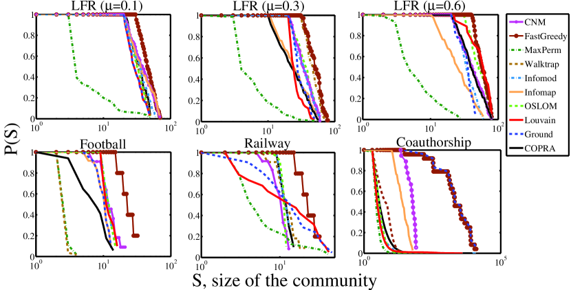
Figure 10: (Color online) Distribution of the community size obtained from the ground-truth structure vis-a-vis other community detection algorithms.

8.7 Detection of small sized communities

Many optimization algorithms tend to ignore smaller size communities and combine them to produce larger communities. This phenomenon is known as the “resolution limit” problem. Here we provide experimental results to show that MaxPerm can mitigate the effects of resolution limit (analytical proof is given in Section 11).

In our test suite, we observe that all the competing algorithms produce larger sized communities as compared to those obtained by permanence. Figure 10 shows the community size distribution of the ground-truth structure, and that obtained from other community detection algorithms. We observe that with the increase of $\mu$ in LFR network, the size distributions obtained from ground-truth and Louvain respectively start separating, while the pattern obtained from MaxPerm remains almost same in that most of the communities are small in size. Interestingly, for coauthorship network even if most of the communities in ground-truth are large in size, the communities obtained from Louvain and MaxPerm are almost of similar size.

We therefore investigate whether these smaller size communities are arbitrary or actually represent different sub-communities of a large community present in the ground-truth structure. As shown in Table 5, for the co-authorship network the smaller communities actually represented sub-disciplines of a larger academic field. However, such meta data is not available for all networks. To answer this question, we construct a bipartite network consisting of the communities obtained from the algorithm $A$ (denoted as set $C_{A}$) as vertices in one partition and the ground-truth communities (denoted as set $C_{G}$) as vertices in another partition. We create the edges $C_{A}\times C_{G}$ with edge weights derived as follows: the weight of the edge connecting $c_{a}\in C_{A}$ and $c_{g}\in C_{G}$ is measured by the fraction of vertices in $c_{a}$ that are also part of $c_{g}$. We only consider edges with non-zero weights. If a detected community is mostly subsumed by one ground-truth community, it produces very high edge-weight (ranging from 0.8-1) and very small-edge-weight (0-0.2); whereas medium edge-weight (0.4-0.7) indicates that the detected community is equally absorbed in multiple ground-truth communities. For example, assume that $c_{a}$ contains 10 nodes which are distributed into two ground-truth communities $c_{g}^{1}$ and $c_{g}^{2}$ in two different ways: (Case 1.) 8 vertices of $c_{a}$ are in $c_{g}^{1}$ and 2 are in $c_{g}^{2}$, (Case 2.) 4 vertices of $c_{a}$ are in $c_{g}^{1}$ and 6 are in $c_{g}^{2}$. Therefore, in Case 1 the edge weights are 0.8 and 0.2 for ($c_{a}\rightarrow c_{g}^{1}$) and ($c_{a}\rightarrow c_{g}^{2}$) respectively; whereas in Case 2 the edge weights are 0.4 and 0.6 for ($c_{a}\rightarrow c_{g}^{1}$) and ($c_{a}\rightarrow c_{g}^{2}$) respectively.

We construct such weighted bipartite graphs separately for all the algorithms. In Figure 11, we divide the edge-weights into 10 buckets such that bucket 1 corresponds to higher-edge weight. Then in y-axis, we plot the fraction of edges falling in each bucket. We observe that while the proportion of edges for baseline algorithms is higher in medium weight zone, for MaxPerm most of the edges either fall in higher weighted buckets or lower-weighted buckets. This indicates that the communities obtained by MaxPerm are indeed subgroups within one larger community, rather than being scattered across multiple communities.

We also observe that despite finding small communities, the largest-size community obtained by MaxPerm best corresponds to the largest ground-truth community. In Table 4, we show for all the networks that the size of the largest communities detected by the other algorithms is much larger than the size of the largest community present in the ground-truth structure. We also measure the maximum similarity (using Jaccard coefficient) between the largest-size community detected by each algorithm with the communities in ground-truth structure and notice that MaxPerm is able to detect largest size community which is most similar to the ground-truth structure (see Table 4). These experimental results indicate that MaxPerm is more effective in reducing the effect of resolution limit.

Communities	Sub-communities
Algorithms	Theory of computation; Formal methods;
and Theory	Information & coding theory;
	Computational geometry; Data structure;
Databases	Models; Query optimization; Database
	languages; storage; Performance;
	security, and availability

Table 5: Example of communities and sub-communities obtained from coauthorship network using MaxPerm algorithm.

Figure 11: (Color online) Fraction of edges of the bipartite network with a specific weight. The range of the edge-weight is divided into ten buckets (bucket 1: 0.9-1, bucket 2: 0.8-0.89 and so on). The bipartite network corresponds to the coauthorship network.

9 Effect of vertex ordering

Most of the community detection algorithms attempt to optimize certain functions (such as modularity) and therefore are heavily dependent on the order in which vertices are processed. This is an important source of concern among researchers on how to reconcile results where the final outcome can change due to the mere change in vertex ordering [Seifi et al. (2013), Lancichinetti and Fortunato (2012b), Delvenne et al. (2010), De Meo et al. (2013b), Chakraborty et al. (2013)]. In this direction, [Chakraborty et al. (2013)] show that despite such fluctuations in the final outcome, there exist few invariant groups of vertices in a network that always remain together, and they are known as “constant communities”. Further, they study the change in community structure based on the number of constant communities by a metric, called sensitivity ($\phi$), which is measured as the ratio of the number of constant communities to the total number of vertices. For a particular network, if the value of $\phi$ for an algorithm remains consistent over different vertex orderings, the algorithm would be qualified to be resilient to the effect of vertex ordering.

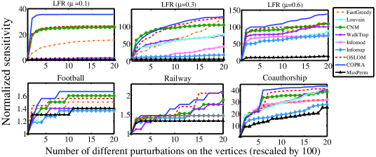
Figure 12: Sensitivity of each algorithm across 2000 permutations. The x-axis is rescaled by a constant factor of 100. Y-axis indicates the value of sensitivity as it changes over the permutations. For better visualization, we rescale the value of sensitivity with the minimum value for each algorithm so that the sensitivity of all the algorithms always starts from 1.

We plot the value of sensitivity over different vertex orderings for each algorithm in Figure 12. In x-axis, we plot the number of different permutations of the vertices. For fair comparison, we normalize the sensitivity values by the minimum value for each algorithm and plot it in y-axis so that the sensitivity profiles of all the algorithms start from 1. For a particular network, the lower the value of sensitivity of an algorithm across different perturbations, the better the algorithm resilient to the initial vertex ordering. There are two consequences of this result: (i) For a specific LFR network, say LFR ($\mu=0.3$), we can observe that MaxPerm remains almost consistent in terms of sensitivity over different iterations, which is in most cases followed by Infomod, Infomap and Louvain. COPRA and OSLOM perform worst among the others. (ii) Across different LFR networks, we observe that with the increase of $\mu$, the performance of all the algorithms start deteriorating. The reason could be that with the increase of $\mu$, communities in LFR network become fuzzier, and therefore multiple community partitions can be equally good. Similar result is observed across different real-world networks where the algorithms tend to be largely insensitive for coauthorship network due to the lack of clear separation between communities.

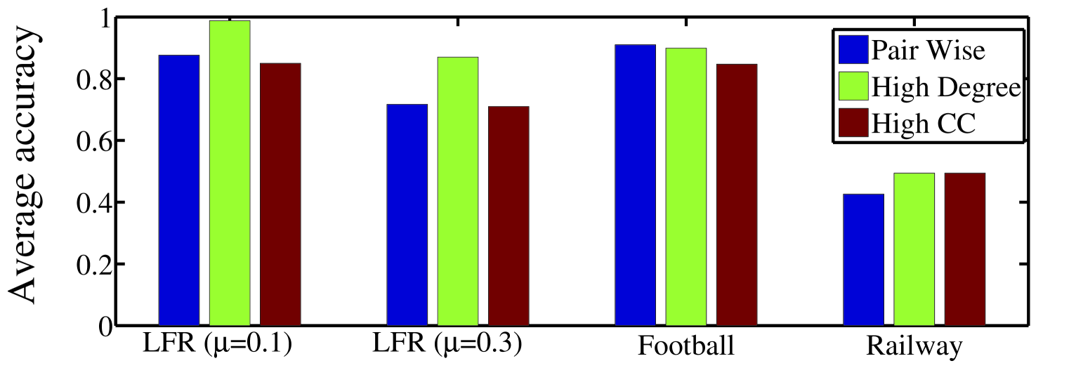
Figure 13: Average accuracy of community detection results with different seeding techniques. Seeding based on high degree gives the highest accuracy.

10 Effect of seed community selection

The first step before starting the iterations to maximize permanence is to place the vertices in initial (seed) communities. The importance of seed communities in detecting communities has been studied for other metrics as in  [Riedy et al. (2011)]. In this section, we explore how it affects the MaxPerm algorithm.

We note that vertices in seed communities should consist of connected subgraphs. If the vertices in the communities are not connected to each other, then their initial permanence will be zero (because $I(v)$ is zero), and moving to a neighboring community does not improve this value. We consider three seed selection strategies as follows:

• Pair Wise: Two vertices are assigned to the same seed community if they are connected by an edge. If we encounter a vertex whose neighbors have all been already assigned to communities, that unmatched vertex is kept as a singleton. This is the fastest out of the three seeding methods.

• High Degree: We first order the vertices in the decreasing order of degree. The vertex with the highest degree and its neighbors are assigned to the same community. We continue combining each unassigned vertex in the sorted list and its unassigned neighbors into a community. This seeding is based on maximizing $I(v)$ for the high degree vertices.

• High CC: We order the vertices in the decreasing order of clustering coefficient, and similar to the high degree, combine the vertices with high clustering coefficient and their neighbors in a community. This seeding is based on maximizing $c_{in}(v)$ and is the most expensive of the three methods.

We test the seeding strategies on the four networks (LFR with $\mu=0.1,0.3$, Football and Railway) on which MaxPerm consistently outperformed the other algorithms. As can be seen in Figure 13, the best accuracy comes from using the high degree strategy. The reason for this is that Pair Wise depends on the vertex ordering, and the pairings can change depending on how vertices are numbered. High CC is too restrictive, because once a vertex is in a tightly coupled group, there is less chance for it to migrate to a larger (if slightly) less tightly coupled group. Thus maximizing permanence using high clustering coefficient tends to fall into local minima. In High Degree, the groupings are less random compared to Pair Wise, but they also provide more flexibility for vertices to migrate between communities as compared to High CC. We believe that this is the reason behind High Degree providing the best accuracy.

11 Handling limitations of modularity maximization algorithms

In this section we analytically show how finding communities by maximizing permanence can reduce the effect of some of the common issues in community detection including (a) resolution limit, (b) degeneracy of solution and (c) dependence on the size of the graph.

We illustrate our proof using a simple example of two communities $A$ and $B$ connected by one vertex $v$ (as shown in Figure 14). There is no edge between the communities $A$ and $B$, except through the vertex $v$. This simple example covers many of the scenarios where problems due to degeneracy of solutions or resolution limits arise. For example, by considering $A$ and $B$ to be cliques, and $v$ to be a vertex within the clique $A$, we can form a subgraph from the circle of cliques as shown in Figure 15(a). This figure is a common example to show the existence of resolution limit [Fortunato and Barthelemy (2007)]. In a similar manner, by considering $A$ and $B$ as single vertices, we can obtain the subgraphs of a grid as shown in Figure 15(b). A grid is an example of a network where multiple solutions can occur.

Case 1: [$(A+v):B$]               Case 2: [$A:(B+v)$]

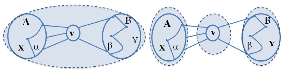
Case 3: [$(A+v+B)$]               Case 4: [$A:B:v$]

Figure 14: (Color online) Illustrative example explaining four possible cases of community assignment of vertex $v$.

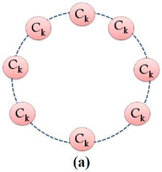
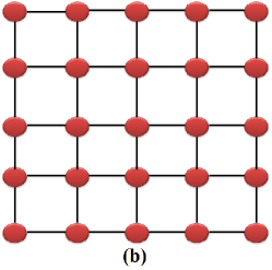
Figure 15: (a) A cycle of $m$ identical $k$-cliques each having $k$ vertices and connected by single edges; (b) a $5\times 5$ grid network.

11.1 Terminology and Theorems

Let vertex $v$ be connected to $\alpha$ ($\beta$) nodes in community $A$ ($B$), and these $\alpha$ ($\beta$) nodes form the set $N_{\alpha}$ ($N_{\beta}$). The number of vertices in community $A$ is ($x+\alpha$), and the number of vertices in community $B$ is ($y+\beta$). Let the average internal degree (connections to internal neighbors only) of a vertex $a\in N_{\alpha}$ and a vertex $b\in N_{\beta}$, before $v$ is added, be $I_{\alpha}$ and $I_{\beta}$ respectively. Let the average internal clustering coefficient of the neighboring nodes in communities $A$ and $B$ be $C_{A}$ and $C_{B}$ respectively.

If $v$ is added to communities $A$ ($B$) then the average internal clustering coefficient of $v$ becomes $C^{v}_{A}$ ($C^{v}_{B}$) respectively, and the average internal clustering coefficients of the nodes in $N_{\alpha}$($N_{\beta}$) become $C^{\alpha}$ ($C^{\beta}$). We will use these average values to approximate the permanence measure.

We assume that the communities $A$ and $B$ are tightly connected internally such that the values of $C_{A}$ and $C_{B}$ are very high (at least greater than 0.5). We note that the values $C^{\alpha}$ ($C^{\beta}$) will depend on the connections of $v$ to the communities and the connections of the vertices in $N_{\alpha}$ and $N_{\beta}$.

To simplify this, we will consider two special cases. One case is when the nodes in the community are tightly connected and adding $v$ does not significantly change the internal clustering coefficient. In this case, we assume $C^{\alpha}=C^{A}$ and $C^{\beta}=C^{B}$. The other case is when $v$ is added that no new connections are formed among the neighbors of $v$, but the internal degree increases by one. Therefore, $C^{\alpha}=C_{A}\frac{(I_{\alpha}-1)}{(I_{\alpha}+1)}$ (similarly, $C^{\beta}=C_{B}\frac{(I_{\beta}-1)}{(I_{\beta}+1)}$ ).

The combination of communities $A$, $B$ and the vertex $v$ can have four cases (see Figure 14) as follows:

• Case 1. $v$ joins with community $A$ only. We denote this configuration as $[(A+v):B]$, and its total permanence as $P_{(A+v):B}$. We assume that the combined permanence of all nodes $x\not\in(N_{\alpha}\cup N_{\beta}\cup v)$ as $P_{x}$. This value will not be affected due to the re-assignments. Therefore, the total permanence is the sum of the following factors: $P_{x}$, $[\alpha C^{\alpha}]$ (for the nodes in $N_{\alpha}$ connected to $v$), $[\frac{\alpha}{(\alpha+\beta)\beta}-(1-C^{v}_{A})]$ (for vertex $v$) and $[\beta(\frac{I_{\beta}}{I_{\beta}+1}-(1-C_{B}))]$ (for the nodes in $N_{\beta}$).
  

  $P_{(A+v):B}=P_{x}+\alpha C^{\alpha}+\frac{\alpha}{(\alpha+\beta)\beta}-(1-C^{v}_{A})+\beta(\frac{I_{\beta}}{I_{\beta}+1}-(1-C_{B}))$
  

• Case 2. $v$ joins with community $B$ only. We denote this configuration as $[(A:(v+B)]$, and its total permanence as $P_{A:(v+B)}$. The values of this total permanence is the sum of the following factors: $P_{x}$, $[\alpha(\frac{I_{\alpha}}{I_{\alpha}+1}-(1-C_{A}))]$ (for the nodes in $N_{\alpha}$), $[\frac{\beta}{(\alpha+\beta)\alpha}-(1-C^{v}_{B})]$ (for vertex $v$) and $[\beta C^{\beta}]$ (for the nodes in $N_{\beta}$ connected to $v$).
  

  $P_{A:(v+B)}=P_{x}+\alpha(\frac{I_{\alpha}}{I_{\alpha}+1}-(1-C_{A}))+\frac{\beta}{(\alpha+\beta)\alpha}-(1-C^{v}_{B})+\beta C^{\beta}$
  

• Case 3. $A$, $B$ and $v$ merge together. We denote this configuration as $[(A+v+B)]$, and its total permanence as $P_{(A+v+B)}$. The values of this total permanence is the sum of the following factors: $P_{x}$, $[\alpha C^{\alpha}]$ (for the nodes in $N_{\alpha}$), $[\frac{\alpha(\alpha-1)C^{v}_{A}+\beta(\beta-1)C^{v}_{B}}{(\alpha+\beta)(\alpha+\beta-1)}]$ (for vertex $v$) and $[\beta C^{\beta}]$ (for the nodes in $N_{\beta}$ connected to $v$).
  

  $P_{(A+v+B)}=P_{x}+\alpha C^{\alpha}+\frac{\alpha(\alpha-1)C^{v}_{A}+\beta(\beta-1)C^{v}_{B}}{(\alpha+\beta)(\alpha+\beta-1)}+\beta C^{\beta}$
  

• Case 4. $A$, $B$ and $v$ remain as separate communities. We denote this configuration as $[(A:v:B)]$, and its total permanence as $P_{(A:v:B)}$. The values of this total permanence is the sum of the following factors: $P_{x}$, $[\alpha(\frac{I_{\alpha}}{I_{\alpha}+1}-(1-C_{A}))]$ (for the nodes in $N_{\alpha}$), 0 (for vertex $v$) and $[\beta(\frac{I_{\beta}}{I_{\beta}+1}-(1-C_{B}))]$ (for the nodes in $N_{\beta}$).
  

  $P_{(A:v:B)}=P_{x}+\alpha(\frac{I_{\alpha}}{I_{\alpha}+1}-(1-C_{A}))+\beta(\frac{I_{\beta}}{I_{\beta}+1}-(1-C_{B}))$
  

We present a set of theorems as to when these conditions will occur. By using these theorems we can analytically show that degeneracy of solutions and resolution limit is reduced when maximizing permanence.

Lemma 1 Given $C^{\alpha}=C_{A}$ and $C^{\beta}=C_{B}$, let $Z1=\frac{\alpha-\beta}{\alpha\beta}+\left(C^{v}_{A}-C^{v}_{B}\right)+\left(\frac{\alpha}{I_{\alpha}+1}-\frac{\beta}{I_{\beta}+1}\right)$. The assignment $[(A+v):B]$ will have a higher permanence than $[A:(v+B)]$, if $Z1>0$ and a lower permanence if $Z1<0$.

Given $C^{\alpha}=C_{A}\frac{(I_{\alpha}-1)}{(I_{\alpha}+1)}$ and $C^{\beta}=C_{B}\frac{(I_{\beta}-1)}{(I_{\beta}+1)}$, let $Z2=\frac{\alpha-\beta}{\alpha\beta}+\left(C^{v}_{A}-C^{v}_{B}\right)+\left(\frac{\alpha(C_{A}+1)}{I_{\alpha}+1}-\frac{\beta(C_{B}+1)}{I_{\beta}+1}\right)$. The assignment $[(A+v):B]$ will have a higher permanence than $[A:(v+B)]$, if $Z2>0$ and a lower permanence if $Z2<0$.

Proof. Here we are comparing between Case 1 and Case 2. The difference in total permanence between these two assignments by assuming $C^{\alpha}=C_{A}$ and $C^{\beta}=C_{B}$ is:

$$\begin{split}P_{(A+v):B}-P_{A:(v+B)}&=\frac{\alpha}{(\alpha+\beta)\beta}+C^{v}_{A}+\beta(\frac{I_{\beta}}{I_{\beta}+1}-1)\\ &-(\alpha(\frac{I_{\alpha}}{I_{\alpha}+1}-1)+\frac{\beta}{(\alpha+\beta)\alpha}+C^{v}_{B})\\ &=\frac{\alpha-\beta}{\alpha\beta}+(C^{v}_{A}-C^{v}_{B})+(\frac{\alpha}{I_{\alpha}+1}-\frac{\beta}{I_{\beta}+1})\\ \end{split}$$

The difference in total permanence between these two assignments by assuming $C^{\alpha}=C_{A}\frac{(I_{\alpha}-1)}{(I_{\alpha}+1)}$ and $C^{\beta}=C_{B}\frac{(I_{\beta}-1)}{(I_{\beta}+1)}$ is:

$$\begin{split}P_{(A+v):B}-P_{A:(v+B)}&=\frac{\alpha}{(\alpha+\beta)\beta}+C^{v}_{A}+\beta(\frac{I_{\beta}}{I_{\beta}+1}-1)\\ &-(\alpha(\frac{I_{\alpha}}{I_{\alpha}+1}-1)+\frac{\beta}{(\alpha+\beta)\alpha}+C^{v}_{B})\\ &=\frac{\alpha-\beta}{\alpha\beta}+(C^{v}_{A}-C^{v}_{B})+(\frac{\alpha(C_{A}+1)}{I_{\alpha}+1}-\frac{\beta(C_{B}+1)}{I_{\beta}+1})\\ \end{split}$$

If this difference is greater than zero then $[(A+v):B]$ will have a higher permanence. If the difference is less than zero then $[A:(v+B)]$ will have higher permanence.

Lemma 2 Joining $v$ to community $A$ gives higher permanence than merging the communities $A$, $B$ and $v$, if (i) $C^{\beta}=C_{B}$, and $X>0$ and (ii) if $C^{\beta}=C_{B}\frac{I_{\beta}-1}{I_{\beta}+1}$ and $X+\beta C_{B}\frac{2}{I_{\beta}+1}>0$; where $X=\frac{\alpha}{(\alpha+\beta)\beta}-\frac{{\beta}}{I_{\beta}+1}-1+\frac{\beta(\beta-1)(C^{v}_{A}+C^{v}_{B})}{(\alpha+\beta)(\alpha+\beta-1)}+\frac{2\alpha\beta C^{v}_{A}}{(\alpha+\beta)(\alpha+\beta-1)}$

Proof. We are comparing Case 1 and Case 3 and in this case $C^{\beta}=C_{B}$. The difference in total permanence is:

$$\begin{split}P_{(A+v):B}-P_{(A+v+B)}&=\frac{\alpha}{(\alpha+\beta)\beta}-1+C^{v}_{A}+\beta(\frac{I_{\beta}}{I_{\beta}+1}-1+C_{B})\\ &-(\frac{\alpha(\alpha-1)C^{v}_{A}+\beta(\beta-1)C^{v}_{B}}{(\alpha+\beta)(\alpha+\beta-1)}+\beta C^{\beta})\\ &\mbox{ Substituiting $C_{B}$ with $C^{\beta}$}\\ &=\frac{\alpha}{(\alpha+\beta)\beta}-1+C^{v}_{A}-\frac{{\beta}}{I_{\beta}+1}\\ &-(\frac{\alpha(\alpha-1)C^{v}_{A}+\beta(\beta-1)C^{v}_{B}}{(\alpha+\beta)(\alpha+\beta-1)})\\ &=\frac{\alpha}{(\alpha+\beta)\beta}-1-\frac{{\beta}}{I_{\beta}+1}\\ &+\frac{\beta(\beta-1)(C^{v}_{A}+C^{v}_{B})}{(\alpha+\beta)(\alpha+\beta-1)}+\frac{2\alpha\beta C^{v}_{A}}{(\alpha+\beta)(\alpha+\beta-1)}\\ \end{split}$$

Now we consider the case where $C^{\beta}=C_{B}\frac{I_{\beta}-1}{I_{\beta}+1}$. The difference in total permanence is:

$$\begin{split}P_{(A+v):B}-P_{(A+v+B)}&=\frac{\alpha}{(\alpha+\beta)\beta}-1+C^{v}_{A}+\beta(\frac{I_{\beta}}{I_{\beta}+1}-1+C_{B})\\ &-(\frac{\alpha(\alpha-1)C^{v}_{A}+\beta(\beta-1)C^{v}_{B}}{(\alpha+\beta)(\alpha+\beta-1)}+\beta C^{\beta})\\ &\mbox{ Substituiting $C^{\beta}=C_{B}\frac{I_{\beta}-1}{I_{\beta}+1}$}\\ &=\frac{\alpha}{(\alpha+\beta)\beta}-1-\frac{{\beta}}{I_{\beta}+1}+\beta C_{B}\frac{2}{I_{\beta}+1}\\ &+\frac{\beta(\beta-1)(C^{v}_{A}+C^{v}_{B})}{(\alpha+\beta)(\alpha+\beta-1)}+\frac{2\alpha\beta C^{v}_{A}}{(\alpha+\beta)(\alpha+\beta-1)}\\ \end{split}$$

Lemma 3 If $C^{\alpha}=C_{A}$ and $C^{\beta}=C_{B}$ then the communities will merge (i.e., $[(A+v+B)]$), rather than remain separate (i.e., $[A:B:C]$).
If $C^{\alpha}=C_{A}\frac{(I_{\alpha}-1)}{(I_{\alpha}+1)}$ $C^{\beta}=C_{B}\frac{(I_{\beta}-1)}{(I_{\beta}+1)}$ and then the communities will merge if:
$\frac{\alpha(\alpha-1)C^{v}_{A}+\beta(\beta-1)C^{v}_{B}}{(\alpha+\beta)(\alpha+\beta-1)}>\alpha\frac{(2C_{A}-1)}{I_{\alpha}+1}+\beta\frac{(2C_{B}-1)}{I_{\beta}+1}$.

Proof: We are comparing Case 3 and Case 4, and the case $C^{\alpha}=C_{A}$ and $C^{\beta}=C_{B}$ The difference in total permanence is:

$$\begin{split}P_{(A+v+B)}-P_{(A:v:B)}&=\alpha C^{\alpha}+\frac{\alpha(\alpha-1)C^{v}_{A}+\beta(\beta-1)C^{v}_{B}}{(\alpha+\beta)(\alpha+\beta-1)}+\beta C^{\beta}\\ &-(\alpha(\frac{I_{\alpha}}{I_{\alpha}+1}-(1-C_{A}))+\beta(\frac{I_{\beta}}{I_{\beta}+1}-(1-C_{B})))\\ &=\frac{\alpha(\alpha-1)C^{v}_{A}+\beta(\beta-1)C^{v}_{B}}{(\alpha+\beta)(\alpha+\beta-1)}\\ &+\frac{\alpha}{I_{\alpha}+1}+\frac{\beta}{I_{\beta}+1}\\ \end{split}$$

This value is always positive so the communities will merge.

We now consider the case where $C^{\alpha}=C_{A}\frac{(I_{\alpha}-1)}{(I_{\alpha}+1)}$ $C^{\beta}=C_{B}\frac{(I_{\beta}-1)}{(I_{\beta}+1)}$ permanence is:

$$\begin{split}P_{(A+v+B)}-P_{(A:v:B)}&=\alpha C^{\alpha}+\frac{\alpha(\alpha-1)C^{v}_{A}+\beta(\beta-1)C^{v}_{B}}{(\alpha+\beta)(\alpha+\beta-1)}+\beta C^{\beta}\\ &-(\alpha(\frac{I_{\alpha}}{I_{\alpha}+1}-(1-C_{A}))+\beta(\frac{I_{\beta}}{I_{\beta}+1}-(1-C_{B})))\\ &=\frac{\alpha(\alpha-1)C^{v}_{A}+\beta(\beta-1)C^{v}_{B}}{(\alpha+\beta)(\alpha+\beta-1)}\\ &-\alpha\frac{(2C_{A}-1)}{I_{\alpha}+1}-\beta\frac{(2C_{B}-1)}{I_{\beta}+1}\\ \end{split}$$

Lemma 4 If $C^{\alpha}=C_{A}$ and $C^{\beta}=C_{B}$ then the communities will remain separate (i.e., $[A:v:B]$) rather than $v$ joining with community $A$ (i.e., $[(A+v):B]$), if $\alpha(\frac{1}{I_{\alpha}+1}+\frac{1}{(\alpha+\beta)\beta})+(C^{v}_{A}-1)<0$.

Otherwise, if $C^{\alpha}=C_{A}\frac{(I_{\alpha}-1)}{(I_{\alpha}+1)}$; $C^{\beta}=C_{B}\frac{(I_{\beta}-1)}{(I_{\beta}+1)}$ and then the communities will remain separate if $\alpha(\frac{1-2C_{A}}{I_{\alpha}+1}+\frac{1}{(\alpha+\beta)\beta})+(C^{v}_{A}-1)<0$.

Proof: We are comparing Case 1 and Case 4 for the case $C^{\alpha}=C_{A}\frac{(I_{\alpha}-1)}{(I_{\alpha}+1)}$; $C^{\beta}=C_{B}\frac{(I_{\beta}-1)}{(I_{\beta}+1)}$. The difference in total permanence is:

$$\begin{split}P_{(A+v):B}-P_{(A:v:B)}&=\alpha C^{\alpha}+\frac{\alpha}{(\alpha+\beta)\beta}-(1-C^{v}_{A})\\ &-(\alpha(\frac{I_{\alpha}}{I_{\alpha}+1}-(1-C_{A}))\\ &=\alpha(\frac{1-2C_{A}}{I_{\alpha}+1})+\frac{\alpha}{(\alpha+\beta)\beta}+(C^{v}_{A}-1)\\ \end{split}$$

If we consider the case $C^{\alpha}=C_{A}$ and $C^{\beta}=C_{B}$, then

$$\begin{split}P_{(A+v):B}-P_{(A:v:B)}&=\alpha C^{\alpha}+\frac{\alpha}{(\alpha+\beta)\beta}-(1-C^{v}_{A})\\ &-(\alpha(\frac{I_{\alpha}}{I_{\alpha}+1}-(1-C_{A}))\\ &=\alpha(\frac{1}{I_{\alpha}+1}+\frac{1}{(\alpha+\beta)\beta})+(C^{v}_{A}-1)\\ \end{split}$$

11.2 Mitigation of issues in modularity maximization

Using the above lemmas, we can determine the conditions for which a particular assignment (of the four possible ones) will give the highest permanence. Using these conditions, we shall show how permanence overcomes three major shortcomings of modularity maximization.

(i) Degeneracy of solution is a problem where a community scoring metric (e.g., modularity) admits multiple distinct high-scoring solutions and typically lacks a clear global maximum, thereby, resorting to tie-breaking [Good et al. (2010)]. Consider the case where the vertex $v$ has equal connections to groups $A$ and $B$, therefore $\alpha$ = $\beta$, and the neighbors of $v$ are not connected to each other, i.e. $C^{\alpha}=C_{A}\frac{(I_{\alpha}-1)}{(I_{\alpha}+1)}$; $C^{\beta}=C_{B}\frac{(I_{\beta}-1)}{(I_{\beta}+1)}$. Since the neighbors are not connected therefore $C^{v}_{A}=C^{v}_{B}=0$.

In this case the condition in Lemma 4 becomes; $P_{(A+v):B}-P_{(A:v:B)}=\alpha\frac{1-2C_{A}}{I_{\alpha}+1}+\frac{1}{2\alpha}-1$ Because the values of $C_{A}$ range from $0$ to $1$, the values of $(1-2C_{A})$ is negative. Moreover $\frac{1}{2\alpha}$ is less than 1. Therefore the value of $P_{(A+v):B}-P_{(A:v:B)}$ is negative, indicating that permanence is higher if $v$, $A$ and $B$ form separate communities.

According to Lemma 3, the communities will merge if:
$\frac{\alpha(\alpha-1)C^{v}_{A}+\beta(\beta-1)C^{v}_{B}}{(\alpha+\beta)(\alpha+\beta-1)}>\alpha\frac{(2C_{A}-1)}{I_{\alpha}+1}+\beta\frac{(2C_{B}-1)}{I_{\beta}+1}$. Since $C^{v}_{A}=C^{v}_{B}=0$, the left hand side is 0. Therefore permanence is higher if $v$, $A$ and $B$ form separate communities.

Therefore, if $v$ has equal number of connections to each community, and the neighbors of $v$ are not connected then $v$ will remain as singleton, rather than arbitrarily joining any of its neighbor groups.

(ii) Resolution limit is a problem where communities of certain small size are merged into larger ones [Fortunato and Barthelemy (2007), Good et al. (2010)]. One of the classic examples where modularity cannot identify communities of small size is a cycle of $m$ cliques (see Figure 15 (a)). Here maximum modularity is obtained if two neighboring cliques are merged.

In the case of permanence, we can determine that whether two communities $A$ and $B$ would merge (as in modularity) or whether $v$ would join community $A$ (we select $A$ as the community to explain the case, but similar analysis can also be done for the case when $v$ joins $B$).

We assume that the communities $A$ and $B$ are tightly connected, such that $C_{A}>.5$ and $C_{B}>.5$. We assume $v$ is tightly connected to group $A$, such that $C^{v}_{A}\approx 1$ and connected by one edge to group $B$ ($\beta=1$), such that $C^{\beta}=C_{B}\frac{I_{\beta}-1}{I_{\beta}+1}$.

From Lemma 2 we have; $P_{(A+v):B}-P_{(A+v+B)}=\frac{\alpha}{(\alpha+1)}-1-\frac{{1}}{I_{\beta}+1}+\frac{2C_{B}}{I_{\beta}+1}+\frac{2}{\alpha+1}$

which is equal to $\frac{1}{(\alpha+1)}+\frac{2C_{B}-1}{I_{\beta}+1}$. Since $C_{B}>.5$ therefore the value is positive. This indicates that permanence is higher if $v$ joins group $A$ rather than if the three groups merge.

Note that, this result is independent of the size of the communities $A$ and $B$. This phenomenon highlights that in general, if $v$ is very tightly connected to a community and very loosely connected to another community, highest permanence is obtained when $v$ joins the community to which it is more connected.

Table 6: Change in modularity, permanence and the other network parameters with the (near-)symmetric growth of coauthorship network as discussed in Section 3.2. $N$: number of nodes, $C$: number of communities, $I$: internal degree, $D$: degree, $c_{in}(v)$: clustering coefficient of $v$ with respect to its internal neighbors, $E_{max}(v)$: maximum external connectivity of $v$, $CD$: average intra-community density (number of edges normalized by the number of nodes). The consistency of four network parameters indicates symmetric growth of the network in different instantiations.

Coauthorship	Network	$N$	964	1515	1991	2681	3386	4836	6284	7814	9001	10386
	properties	$C$	24	24	24	24	24	24	24	24	24	24
		$\frac{I}{D}$	0.082	0.095	0.093	0.091	0.089	0.104	0.111	0.112	0.115	0.113
		$\frac{1}{E_{max}(v)}$ ($\times 10^{-4}$)	3.8	3.2	2.9	3.9	2.8	2.11	2.39	2.92	2.69	3.22
		$1-c_{in}(v)$	0.239	0.248	0.246	0.251	0.251	0.260	0.265	0.269	0.270	0.274
		$CD$	74.30	80.30	90.34	98.18	102.68	118.68	118.72	123.29	110.22	123.292
	Modularity		0.369	0.374	0.395	0.392	0.421	0.422	0.465	0.471	0.493	0.501
	Permanence		0.094	0.092	0.092	0.096	0.095	0.095	0.097	0.097	0.097	0.098

(iii) Asymptotic growth of value of a metric implies a strong dependence on both the size of the network and the number of modules the network contains [Good et al. (2010)]. Rewriting equation 1, we get the permanence of the entire network $G$ as follows: $Perm(G)=\frac{1}{|V|}\sum_{v\in V}\left[\frac{I(v)}{D(v)E_{max}(v)}\right]-\frac{1}{|V|}\sum_{v\in V}\left[(1-c_{in}(v))\right]$. We can notice that most of the parameters in the above formula are independent of the symmetric growth of network size and the number of communities. Table 6 illustrates the property from a real-life example of coauthorship network where the modularity increases with increase in the size of the network, while permanence remains almost constant.

12 Conclusion and Future Work

In this paper, we present a new vertex-centric community quality metric, called permanence, that unlike other metrics considers both the connection density among internal neighbors and the distribution of external connectivity of a vertex. We empirically demonstrated on synthetic and real-world networks that permanence is an effective community evaluation metric compared to other well-known approaches such as modularity, conductance and cut-ratio. We also showed how permanence is appropriately sensitive to the fluctuations of community structure. Further experiments on characterizing permanence revealed that – (i) permanence can measure the persistence of a vertex in its own community, and (ii) one can strengthen the community structure by suitably removing nodes with low permanence value. Finally, we developed a new community detection algorithm by maximizing permanence - MaxPerm that has a much superior performance compared to state-of-the art algorithms on most datasets. Moreover, MaxPerm detects more efficient and realistic community structure – (i) the obtained communities are highly connected, irrespective of the size of the communities, as a result of which one is able to detect small and even singleton communities; (ii) the communities obtained by MaxPerm are less affected by the initial vertex ordering.

The proposed metric calls for deeper levels of investigation. More algorithms and datasets from diverse areas need to be selected to reinforce the robustness of our proposed metric. Since permanence is a local metric, one immediate direction would be to discover local community boundary for a particular seed node. We intend to extend permanence metric to enable evaluation of the quality of overlapping community structures and to weighted and directed networks. Overall, we believe that this metric will help in formulating a strong theoretical foundation in the identification and evaluation of various types of community strictures where the ground-truth is not known.

APPENDIX

In this appendix, we expand Table 2. In this table, the differences between the results obtained from MaxPerm and all the other algorithms are shown in terms of six validation measures for all the networks.

Table 7: Differences of MaxPerm with the other algorithms in terms of the validation metrics. Positive differences indicate the improvement of our algorithm. The rows indicated by “L” show values obtained from the LFR graphs with $\mu=$0.1, 0.3 and 0.6 respectively (from left to right and separated by semicolons). The rows indicated by “R” show values for football, railway and coauthorship networks (from left to right and separated by semicolons). The average improvements over different validation measures are shown in rows 8 and 15 for LFR and real-world networks respectively.

Type	Validation	Louvain	FastGreedy	CNM	WalkTrap	Infomod	Infomap	COPRA	OSLOM
	metrics
L	NMI	0.14; 0.00; -0.78	0.00; 0.81; -0.02	0.07; 0.24; -0.25	0.00; 0.00; -0.13	0.04; 0.05; -0.78	0.00; 0.01; 0.12	0.08; 0.09; -0.78	0.00; 0.01; 0.12
	ARI	0.00; -0.02; -0.76	0.00; 0.98; 0.03	0.24; 0.59; -0.10	0.00; 0.01; -0.52	0.11; 0.13; -0.05	0.00; -0.01; -0.95	0.16; 0.01; 0.02	0.00; -0.01; -0.86
	PU	0.00; 0.00; -0.72	0.00; 0.86; 0.04	0.12; 0.41; -0.13	0.00; -0.01; -0.58	0.08; 0.09; -0.11	0.00; 0.00; -0.83	0.09; -0.01; 0.06	0.00; 0.01; -0.81
	W-NMI	0.00; 0.00; -0.78	0.00; 0.81; 0.01	0.06; 0.23; -0.10	0.00; 0.00; -0.58	0.02; 0.04; -0.08	0.00; 0.00; -0.94	0.07; 0.03; 0.04	0.00; 0.00; -0.88
	W-ARI	0.00; 0.02; -0.72	0.00; 0.93; 0.07	0.23; 0.54; -0.04	0.00; -0.01; -0.52	0.05; 0.08; -0.02	0.00; -0.01; -0.88	0.16; -0.01; 0.10	0.00; -0.01; -0.82
	W-PU	0.00; 0.00; -0.79	0.00; 0.86; 0.00	0.11; 0.39; -0.20	0.00; 0.00; -0.67	0.05; 0.09; -0.18	0.00; 0.00; -0.89	0.09; 0.00; 0.01	0.00; 0.00; -0.88
	Avg.	0.02; 0.00; -0.75	0.00; 0.87; 0.02	0.14; 0.40; -0.13	0.00; 0.00; -0.50	0.06; 0.08; -0.20	0.00; 0.00; -0.72	0.11; 0.02; -0.09	0.00; 0.00; -0.68
R	NMI	0.01; 0.37; 0.03	0.00; 0.14; 0.13	0.22; 0.07; 0.02	0.01; 0.11; 0.01	0.01; 0.25; -0.02	0.01; 0.06; -0.06	0.02; 0.05; 0.14	0.03; 0.16; 0.09
	ARI	0.00; 0.04; -0.08	0.00; 0.36; 0.13	0.42; -0.09; 0.02	0.03; -0.07; 0.08	0.03; 0.05; -0.01	0.04; -0.06; -0.05	0.09; -0.06; 0.12	-0.06; 0.01; 0.05
	PU	-0.01; 0.08; -0.10	-0.01; 0.41; 0.13	0.26; 0.11; 0.12	0.05; 0.07; 0.05	0.02; 0.13; -0.01	-0.02; 0.06; -0.06	0.04; 0.06; 0.07	-0.04; 0.11; 0.06
	W-NMI	0.07; 0.27; 0.05	0.02; 0.56; 0.18	0.37; 0.10; 0.05	0.05; 0.14; 0.07	0.05; 0.43; -0.06	0.03; 0.17; -0.01	0.04; 0.14; 0.02	0.03; 0.28; 0.12
	W-ARI	0.02; 0.05; 0.05	0.00; 0.31; 0.11	0.34; -0.15; 0.02	0.02; -0.11; 0.05	0.02; 0.17; -0.06	0.00; -0.07; -0.01	0.01; -0.10; 0.09	0.00; 0.05; 0.11
	W-PU	0.01; 0.05; 0.02	0.06; 0.44; 0.14	0.21; -0.06; 0.06	-0.05; -0.04; -0.15	-0.05; 0.12; -0.12	-0.06; -0.05; 0.05	0.00; -0.05; 0.08	-0.06; 0.00; 0.10
	Avg.	0.02; 0.14; 0.00	0.01; 0.37; 0.14	0.30; 0.00; 0.05	0.02; 0.02; 0.02	0.01; 0.19; -0.04	0.00; 0.02; -0.02	0.03; 0.01; 0.09	-0.01; 0.11; 0.09

References

- [1]
- Ahn et al. (2010) Yong-Yeol Ahn, James P. Bagrow, and Sune Lehmann. 2010. Link communities reveal multiscale complexity in networks. Nature 466 (August 2010), 761–764.
- Arenas et al. (2008) A Arenas, A Fernández, and S Gómez. 2008. Analysis of the structure of complex networks at different resolution levels. New Journal of Physics 10, 5 (2008), 053039.
- Bader et al. (2013) David A. Bader, Henning Meyerhenke, Peter Sanders, and Dorothea Wagner (Eds.). 2013. Graph Partitioning and Graph Clustering - 10th DIMACS Implementation Challenge Workshop, Georgia Institute of Technology, Atlanta, GA, USA, February 13-14, 2012. Proceedings. Contemporary Mathematics, Vol. 588. American Mathematical Society.
- Baumes et al. (2005) Jeffrey Baumes, Mark Goldberg, and Malik Magdon-Ismail. 2005. Efficient identification of overlapping communities. In Proceedings of the 2005 IEEE international conference on Intelligence and Security Informatics (ISI’05). Springer-Verlag, Berlin, Heidelberg, 27–36.
- Berry et al. (2011) Jonathan W. Berry, Bruce Hendrickson, Randall A. LaViolette, and Cynthia A. Phillips. 2011. Tolerating the community detection resolution limit with edge weighting. Physical Review E 83, 5 (May 2011), 056119.
- Blondel et al. (2008) Vincent D Blondel, Jean-Loup Guillaume, Renaud Lambiotte, and Etienne Lefebvre. 2008. Fast unfolding of communities in large networks. J. Stat. Mech (2008), P10008.
- Chakrabort et al. (2013) Tanmoy Chakrabort, Sandipan Sikdar, Vihar Tammana, Niloy Ganguly, and Animesh Mukherjee. 2013. Computer Science Fields As Ground-truth Communities: Their Impact, Rise and Fall. In Proceedings of the 2013 IEEE/ACM International Conference on Advances in Social Networks Analysis and Mining (ASONAM ’13). ACM, New York, NY, USA, 426–433.
- Chakraborty (2015) Tanmoy Chakraborty. 2015. Leveraging disjoint communities for detecting overlapping community structure. Journal of Statistical Mechanics: Theory and Experiment 2015, 5 (2015), P05017. http://stacks.iop.org/1742-5468/2015/i=5/a=P05017
- Chakraborty et al. (2016a) Tanmoy Chakraborty, Ayushi Dalmia, Animesh Mukherjee, and Niloy Ganguly. 2016a. Metrics for Community Analysis: A Survey. CoRR abs/1604.03512 (2016).
- Chakraborty et al. (2016b) Tanmoy Chakraborty, Suhansanu Kumar, Niloy Ganguly, Animesh Mukherjee, and Sanjukta Bhowmick. 2016b. GenPerm: A Unified Method for Detecting Non-overlapping and Overlapping Communities. CoRR abs/1604.03454 (2016).
- Chakraborty et al. (2013) Tanmoy Chakraborty, Sriram Srinivasan, Niloy Ganguly, Sanjukta Bhowmick, and Animesh Mukherjee. 2013. Constant Communities in Complex Networks. Scientific Reports 3 (May 2013).
- Chakraborty et al. (2014) Tanmoy Chakraborty, Sriram Srinivasan, Niloy Ganguly, Animesh Mukherjee, and Sanjukta Bhowmick. 2014. On the Permanence of Vertices in Network Communities. In Proceedings of the 20th ACM SIGKDD International Conference on Knowledge Discovery and Data Mining (KDD ’14). ACM, New York, NY, USA, 1396–1405. DOI:http://dx.doi.org/10.1145/2623330.2623707
- Chen et al. (2013) Mingming Chen, Tommy Nguyen, and Boleslaw Szymanski. 2013. A New Metric for Quality of Network Community Structure. ASE Human Journal 1, 4 (2013), 226–240.
- Chierichetti et al. (2010) Flavio Chierichetti, Silvio Lattanzi, and Alessandro Panconesi. 2010. Rumour Spreading and Graph Conductance. In SODA. SIAM, 1657–1663. http://www.siam.org/proceedings/soda/2010/SODA10_135_chierichettif.pdf
- Clauset et al. (2004) Aaron Clauset, M. E. J. Newman, , and Cristopher Moore. 2004. Finding community structure in very large networks. Phys. Rev. E 70, 6 (2004), 066111.
- Danon et al. (2005) L. Danon, A. Diaz-Guilera, J. Duch, and A. Arenas. 2005. Comparing community structure identification. Journal of Statistical Mechanics: Theory and Experiment 9 (2005), P09008.
- De Meo et al. (2013a) Pasquale De Meo, Emilio Ferrara, Giacomo Fiumara, and Alessandro Provetti. 2013a. Enhancing community detection using a network weighting strategy. Journal of Information Science 222 (Feb. 2013), 648–668.
- De Meo et al. (2013b) Pasquale De Meo, Emilio Ferrara, Giacomo Fiumara, and Alessandro Provetti. 2013b. Enhancing Community Detection Using a Network Weighting Strategy. Inf. Sci. 222 (Feb. 2013), 648–668. DOI:http://dx.doi.org/10.1016/j.ins.2012.08.001
- Delvenne et al. (2010) J.-C. Delvenne, S. N. Yaliraki, and M. Barahona. 2010. Stability of graph communities across time scales. Proceedings of the National Academy of Sciences 107, 29 (2010), 12755–12760.
- Demers et al. (1987) Alan Demers, Dan Greene, Carl Hauser, Wes Irish, John Larson, Scott Shenker, Howard Sturgis, Dan Swinehart, and Doug Terry. 1987. Epidemic Algorithms for Replicated Database Maintenance. In PODC. New York, USA, 1–12.
- Evans and Lambiotte (2009) T. S. Evans and R. Lambiotte. 2009. Line graphs, link partitions, and overlapping communities. Phys. Rev. E 80, 1 (July 2009), 016105.
- Farkas et al. (2007) Illés Farkas, Dániel Ábel, Gergely Palla, and Tamás Vicsek. 2007. Weighted network modules. New Journal of Physics 9, 6 (2007), 180.
- Fortunato (2010) Santo Fortunato. 2010. Community detection in graphs. Physics Reports 486, 3-5 (2010), 75 – 174. http://www.sciencedirect.com/science/article/B6TVP-4XPYXF1-1/2/99061fac6435db4343b2374d26e64ac1
- Fortunato and Barthelemy (2007) Santo Fortunato and M Barthelemy. 2007. Resolution limit in community detection. PNAS (Jan. 2007).
- Ghosh et al. (2011) Saptarshi Ghosh, Avishek Banerjee, Naveen Sharma, Sanket Agarwal, and Niloy Ganguly. 2011. Statistical Analysis of The Indian Railway Network: a Complex Network Approach. Acta Physica Polonica B Proceedings Supplement 4 (March 2011), 123–137.
- Girvan and Newman (2002) M. Girvan and M. E. Newman. 2002. Community structure in social and biological networks. PNAS 99, 12 (June 2002), 7821–7826.
- Good et al. (2010) B.H. Good, Y.A. De Montjoye, and A. Clauset. 2010. Performance of modularity maximization in practical contexts. Phys. Rev. E 81, 4 (2010), 046106.
- Guimera and Amaral (2005) Roger Guimera and Luis A. Nunes Amaral. 2005. Functional cartography of complex metabolic networks. Nature 433, 7028 (Feb 2005), 895–900.
- He et al. (2013) Dongxiao He, Dayou Liu, Weixiong Zhang, Di Jin, and Bo Yang. 2013. Discovering link communities in complex networks by exploiting link dynamics. CoRR abs/1303.4699 (2013).
- Holland and Leinhardt (1971) Paul W Holland and Samuel Leinhardt. 1971. Transitivity in Structural Models of Small Groups. Small Group Research 2, 2 (1971), 107–124.
- Hubert and Arabie (1985) L. Hubert and P. Arabie. 1985. Comparing partitions. Journal of classification 2, 1 (1985), 193–218.
- Kannan et al. (2000) R. Kannan, S. Vempala, and A. Veta. 2000. On Clusterings-good, Bad and Spectral. In Proceedings of the 41st Annual Symposium on Foundations of Computer Science (FOCS ’00). IEEE Computer Society, Washington, DC, USA, 367–. http://dl.acm.org/citation.cfm?id=795666.796585
- Kempe et al. (2003) David Kempe, Jon Kleinberg, and Éva Tardos. 2003. Maximizing the Spread of Influence Through a Social Network. In Proceedings of the Ninth ACM SIGKDD International Conference on Knowledge Discovery and Data Mining (KDD ’03). ACM, New York, NY, USA, 137–146. DOI:http://dx.doi.org/10.1145/956750.956769
- Lambiotte (2010) Renaud Lambiotte. 2010. Multi-scale modularity in complex networks.. In WiOpt. IEEE, 546–553.
- Lancichinetti and Fortunato (2009) Andrea Lancichinetti and Santo Fortunato. 2009. Benchmarks for testing community detection algorithms on directed and weighted graphs with overlapping communities. Phys. Rev. E 80, 1 (July 2009), 016118.
- Lancichinetti and Fortunato (2011) Andrea Lancichinetti and Santo Fortunato. 2011. Limits of modularity maximization in community detection. Phys. Rev. E 84 (2011), 066122.
- Lancichinetti and Fortunato (2012a) Andrea Lancichinetti and Santo Fortunato. 2012a. Consensus clustering in complex networks. Scientific Reports 2 (2012).
- Lancichinetti and Fortunato (2012b) Andrea Lancichinetti and Santo Fortunato. 2012b. Consensus clustering in complex networks. CoRR abs/1203.6093 (2012). http://dblp.uni-trier.de/db/journals/corr/corr1203.html#abs-1203-6093
- Lancichinetti et al. (2009) Andrea Lancichinetti, Santo Fortunato, and János Kertész. 2009. Detecting the overlapping and hierarchical community structure in complex networks. New Journal of Physics 11, 3 (2009), 033015.
- Lancichinetti et al. (2010) Andrea Lancichinetti, Filippo Radicchi, Jose J. Ramasco, and Santo Fortunato. 2010. Finding statistically significant communities in networks. CoRR abs/1012.2363 (2010).
- Leicht and Newman (2008) E. A. Leicht and M. E. J. Newman. 2008. Community Structure in Directed Networks. Phys. Rev. Lett. 100, 11 (March 2008), 118703.
- Leskovec et al. (2009) Jure Leskovec, Kevin J. Lang, Anirban Dasgupta, and Michael W. Mahoney. 2009. Community Structure in Large Networks: Natural Cluster Sizes and the Absence of Large Well-Defined Clusters. Internet Mathematics 6, 1 (2009), 29–123.
- Leskovec et al. (2010) Jure Leskovec, Kevin J. Lang, and Michael Mahoney. 2010. Empirical comparison of algorithms for network community detection. In Proceedings of the 19th international conference on World wide web (WWW ’10). ACM, New York, NY, USA, 631–640.
- Manning et al. (2008) Christopher D. Manning, Prabhakar Raghavan, and Hinrich Schütze. 2008. Introduction to Information Retrieval. Cambridge University Press, New York, NY, USA.
- Newman (2006) M E Newman. 2006. Modularity and community structure in networks. PNAS 103, 23 (June 2006), 8577–8582.
- Newman (2003) M. E. J. Newman. 2003. Mixing patterns in networks. Phys. Rev. E 67, 2 (Feb. 2003), 026126. DOI:http://dx.doi.org/10.1103/PhysRevE.67.026126
- Newman (2004a) M. E. J. Newman. 2004a. Analysis of weighted networks. Phys. Rev. E 70, 5 (Nov. 2004), 056131.
- Newman (2004b) M. E. J. Newman. 2004b. Fast algorithm for detecting community structure in networks. Phys. Rev. E 69, 6 (June 2004), 066133.
- Newman (2013) M. E. J. Newman. 2013. Community detection and graph partitioning. CoRR abs/1305.4974 (2013).
- Newman and Girvan (2004) M. E. J. Newman and M. Girvan. 2004. Finding and evaluating community structure in networks. Phys. Rev. E 69, 026113 (2004).
- Orman et al. (2012) Günce Keziban Orman, Vincent Labatut, and Hocine Cherifi. 2012. Comparative Evaluation of Community Detection Algorithms: A Topological Approach. CoRR abs/1206.4987 (2012).
- Palla et al. (2005) Gergely Palla, Imre Derényi, Illés Farkas, and Tamás Vicsek. 2005. Uncovering the overlapping community structure of complex networks in nature and society. Nature 435, 7043 (June 2005), 814–818.
- Pons and Latapy (2006) Pascal Pons and Matthieu Latapy. 2006. Computing Communities in Large Networks Using Random Walks. Journal of Graph Algortihms and Applications 10, 2 (2006), 191–218.
- Psorakis et al. (2011) Ioannis Psorakis, Stephen Roberts, Mark Ebden, and Ben Sheldon. 2011. Overlapping community detection using Bayesian non-negative matrix factorization. Phys. Rev. E 83, 6 (June 2011), 066114.
- Raghavan et al. (2007a) Usha Nandini Raghavan, Reka Albert, and Soundar Kumara. 2007a. Near linear time algorithm to detect community structures in large-scale networks. Phys. Rev. E 76 (Sep 2007), 036106.
- Raghavan et al. (2007b) Usha N. Raghavan, Réka Albert, and Soundar Kumara. 2007b. Near linear time algorithm to detect community structures in large-scale networks. Phys. Rev. E 76, 3 (Sept. 2007), 036106.
- Reichardt and Bornholdt (2006) J. Reichardt and S. Bornholdt. 2006. Statistical mechanics of community detection. Arxiv preprint cond-mat/0603718 (2006).
- Richardson et al. (2009) Thomas Richardson, Peter J. Mucha, and Mason A. Porter. 2009. Spectral tripartitioning of networks. Phys. Rev. E 40 (2009), 027104.
- Riedy et al. (2011) Jason Riedy, David A. Bader, Karl Jiang, Pushkar Pande, and Richa Sharma. 2011. Detecting Communities from Given Seeds in Social Networks. Technical Report GT-CSE-11-01. Georgia Institute of Technology.
- Rosvall and Bergstrom (2007) M. Rosvall and C.T. Bergstrom. 2007. An information-theoretic framework for resolving community structure in complex networks. PNAS 104, 18 (2007), 7327.
- Rosvall and Bergstrom (2008) Martin Rosvall and Carl T. Bergstrom. 2008. Maps of random walks on complex networks reveal community structure. PNAS 105, 4 (2008), 1118–1123.
- Seifi et al. (2013) Massoud Seifi, Ivan Junier, Jean-Baptiste Rouquier, Svilen Iskrov, and Jean-Loup Guillaume. 2013. Stable Community Cores in Complex Networks. In Complex Networks, Ronaldo Menezes, Alexandre Evsukoff, and Marta C. González (Eds.). Studies in Computational Intelligence, Vol. 424. Springer Berlin Heidelberg, 87–98. DOI:http://dx.doi.org/10.1007/978-3-642-30287-9_10
- Shi and Malik (2000) Jianbo Shi and Jitendra Malik. 2000. Normalized Cuts and Image Segmentation. IEEE Trans. Pattern Anal. Mach. Intell. 22, 8 (Aug. 2000), 888–905. DOI:http://dx.doi.org/10.1109/34.868688
- Sun et al. (2011) Peng-Gang Sun, Lin Gao, and Shan Shan Han. 2011. Identification of overlapping and non-overlapping community structure by fuzzy clustering in complex networks. Inf. Sci. 181, 6 (2011), 1060–1071.
- Xie and Szymanski (2011) Jierui Xie and Boleslaw K. Szymanski. 2011. Community Detection Using A Neighborhood Strength Driven Label Propagation Algorithm. CoRR abs/1105.3264 (2011).
- Xie and Szymanski (2012) Jierui Xie and Boleslaw K. Szymanski. 2012. Towards Linear Time Overlapping Community Detection in Social Networks. CoRR abs/1202.2465 (2012).
- Yang and Leskovec (2012) Jaewon Yang and Jure Leskovec. 2012. Defining and evaluating network communities based on ground-truth. In Proceedings of the ACM SIGKDD Workshop on Mining Data Semantics (MDS ’12). ACM, New York, NY, USA, 3:1–3:8.
- Yang and Leskovec (2014) Jaewon Yang and Jure Leskovec. 2014. Overlapping Communities Explain Core-Periphery Organization of Networks. Proceedings of IEEE 102 (2014), 1892 – 1902.