What is the Best Feature Learning Procedure in Hierarchical Recognition Architectures?

Abstract

NOTE: This paper was written in November 2011 and never published. It is posted on arXiv.org in its original form in April 2016.
Many recent object recognition systems have proposed using a two phase training procedure to learn sparse convolutional feature hierarchies: unsupervised pre-training followed by supervised fine-tuning. Recent results suggest that these methods provide little improvement over purely supervised systems when the appropriate nonlinearities are included. This paper presents an empirical exploration of the space of learning procedures for sparse convolutional networks to assess which method produces the best performance. In our study, we introduce an augmentation of the Predictive Sparse Decomposition method that includes a discriminative term (DPSD). We also introduce a new single phase supervised learning procedure that places an L1 penalty on the output state of each layer of the network. This forces the network to produce sparse codes without the expensive pre-training phase. Using DPSD with a new, complex predictor that incorporates lateral inhibition, combined with multi-scale feature pooling, and supervised refinement, the system achieves a 70.6% recognition rate on Caltech-101. With the addition of convolutional training, a 77% recognition was obtained on the CIfAR-10 dataset. The surprising result is that networks using our purely supervised method with a simple encoder and multi-scale pooling produced competitive results, while being significantly simpler and faster to train. This suggests that even task-oriented pre-training may not provide sufficient improvement to justify its use. We conclude with a set of experiments that show an important role of the local contrast normalization in object recognition. We show that including the nonlinearity preserves more information about the input in the output feature maps leading to better discriminability among object categories.

1 Introduction

Over the past few years there has been considerable interest in learning sparse convolutional features for hierarchical recognition architectures, such as feed-forward convolutional networks (or ConvNets) [12, 7, 9, 23, 24], deconvolutional networks[28], and various forms of Restricted Boltzmann Machines stacked to form convolutional feature extractors [13, 14]. Most of these authors advocate the use of a purely unsupervised phase to train the features, optionally followed by a global supervised refinement. However, a surprising set of results in [7] suggests that, on dataset with very few labelled samples such as Caltech-101, learning the features (unsupervised or supervised) seems to bring a relatively modest improvement over using completely random features, provided that a suitable set of non-linearities is used at each stage in the system (local mean removal and contrast normalization). Other results suggest that when the number of labelled samples grows, the unsupervised pre-training phase doesn’t bring a significant improvement over a purely supervised procedure. Furthermore, while the learned filters at the first level seem fairly generic and task independent (oriented Gabors), it is unclear whether the mid-level features would not produce better results by being pre-trained in a somewhat more task-specific manner.

Some recent works have advocated the use of sparse auto-encoders to pre-train feature extractors in an unsupervised manner [7, 9]. In their Predictive Sparse Decomposition method (PSD), and its convolutional version, a non-linear feed-forward encoder function is trained to produce approximations to the sparse codes that best reconstruct the inputs under a sparsity penalty.

This paper startes with this basic approach and presents an empirical exploration of the space of learning procedures for sparse convolutional networks to assess which method produces the best performance. We study 1) a newly introduced discriminative version of PSD (DPSD), 2) a newly introduced single phase supervised training method, 3) convolutional versus patch based unsupervised learning, 4) the effect of using complex encoders that better predict the sparse code, 5) the use of a new multiresolution pooling method, and finally 6) contrast normalization’s role in preserving information about about the input in the high level feature maps.

Results are reported on Caltech-101 that are close to the best methods that use a single feature type. Record results are reported on the CIfAR-10 dataset.

In order to study the effectiveness of task-oriented sparse coding methods, we introduce an augmentation of the PSD  [7, 9] algorithm that includes a discriminative term in the objective function (DPSD). This allows us to directly evaluate the contribution of the discriminative term by comparing the performance of networks pretrained with the respective algorithms. In order to study the effectiveness of pre-training altogether, we present a new purely supervised training method that places an L1 penalty on the output states of randomly initialized networks. This additional regularization drives the network towards producing sparse output maps and the resulting weight configuration resembles the structure that results from DPSD. We refer to this method as sparse-state supervised training. We further compare the traditional patch based DPSD with a version of DPSD that is trained convolutionally over large image regions [9], rather than on isolated patches. Training convolutionally allows the system to take advantage of shifted versions of all the filters to reconstruct images. This greatly reduces redundancies and allows the resulting code to be much sparser. We also test two different predictors in order to determine how important accurate approximations to the optimal sparse codes are for performance. The simple encoder is the same used in  [7]. We then introduce a new predictor architecture that incorporates a kind of lateral inhibition matrix following a linear filter bank and a shrinking function. This matrix is akin to the negative Gramm matrix of the filters used in the ISTA and FISTA algorithms for sparse coding [5]. This new encoder produces very accurate predictions [5], at the expense of additional computation. The encoder—pretrained or randomly initialized— is followed by a rectification, a local mean cancellation, a local contrast normalization, and a spatial feature pooling. To augment the pooling stage, we introduce a new pooling scheme that produces a multiresolution pyramid of features pooled over spatial neighborhoods of different sizes. Lastly, we show that the effect of including the contrast normalization nonlinearity in an object recognition system is to preserve more information about the input image in the output feature maps. This is counter-intuitive, as normalization could be thought of as removing the total signal energy information.

2 Learning Discriminative Dictionaries

We consider the general model

$$\min_{z}E(z)\equiv H(z)+G(z)$$ (1)

where $H(.)$ is a smooth convex function that is continuously differentiable and $G(.)$ is a continuous convex function that is possibly nonsmooth. In recent years, there have been a number of methods developed to solve this general model, such as the Iterative Shrinking and Thresholding Algorithm (ISTA) [4], or its accelerated extension FISTA [2]. The $L_{1}$ regularization problem is a popular special instance of this model where $H(z):=||x-Dz||^{2}$ and $G(z):=||z||_{1}$. In the case of classical sparse coding we have the energy function:

$$E(x,z,D)=||x-Dz||^{2}_{2}+\lambda_{1}||z||_{1}$$ (2)

where $D\in\mathbb{R}^{m\times n}$ is the dictionary (generally overcomplete), $x$ is input signal, $z$ is the sparse code representing $x$, and $\lambda_{1}$ is a hyperparameter controlling the degree of sparsity. For a given input $x$, sparse coding finds the optimal code $z$ that minimizes $E(x,z,D)$. In classical sparse coding, $D$ is hand picked for the task, e.g. (DCT, wavelet, or Gabors) [20], but the recent interest in sparse coding revolves around the ability to learn an appropriate dictionary matrix from data [21]. Dictionary learning for image feature extraction has recently led to state-of-the-art results in image denoising [19] and image classification (see  [3, 7, 17, 23] to name a few).

Learning the dictionary allows us to adapt $D$ to the statistics of the input signal, but it also allows us to enforce task-dependent constraints [18, 17, 16, 3]. If, for example, the objective is image classification and labelled samples are available, then dictionaries can be learned that are both reconstructive and discriminative. Basic reconstructive sparse coding with a learned dictionary minimizes

$${\cal L}(D)=\sum_{i=1}^{m}\min_{z}E(x^{i},z,D)$$ (3)

where $x^{i},\;i=1\ldots m$ is a set of unlabelled training samples. Considering the ability to enforce task dependence, [18] proposed adding a discriminative term, ${\cal C}(y^{i},l(z^{i},\theta))$, where $y^{i}$ is the label of sample $x^{i}$, $l(.)$ is a (linear) discriminant function, ${\cal C}(.)$ is some classification loss function, and $z^{i}$ is the optimal sparse code for $x^{i}$. Incorporating this term leads to the a redefined energy function per sample $i$:

$$E(x,y,z,D,\theta)={\cal C}(y,l(z,\theta))+||x-Dz||^{2}_{2}+\lambda_{1}||z||_{1}$$ (4)

The loss function for learning is ${\cal L}(D,\theta)=\sum_{i=1}^{m}\min_{z}E(x^{i},y^{i},z,D,\theta)$, which is jointly minimized with respect to $D$ and $\theta$.

3 Predictors

In this section, we show how to use a trainable, non-linear, feed-forward predictor to extend the use of discriminative dictionaries to a larger class of recognition systems. In particular we show how we can use this trainable module as a component in a larger, globally-trained system with a flexible, multi-stage architecture.

Following the PSD method [8, 9, 5] we use an encoder to approximate the optimal sparse code, $z^{*}$. This allows the computation of some $\hat{z}\approx z^{*}$ with a rapid-feedforward pass through the encoder, instead of using an iterative procedure to infer the optimal code. In [7] the function used to approximate the $k$-th component of the code was

$$F_{\tanh}(x)_{k}\equiv g_{k}\tanh\left(W_{k}.x+b_{k}\right)$$ (5)

where $F_{\tanh}(x)_{k}$ is the $k$-th output, $g_{k}$ is a scalar gain, $W_{k}$ is a the $k$-th dictionary element. The use of this function is not particularly well justified, given that it makes it difficult to produce outputs near zero. The only rationales seem to be that it is similar to non-linear functions used in traditional neural nets, and that it seems to yield easy convergence and reasonable recognition performance.

To address this, we also investigate the effect of using a richer encoder based on the Iterative Shrinking and Thresholding Algorithm (ISTA) for sparse coding  [4, 2] (see  [5] for details). The function used to approximate the sparse code was

$$F_{si}(x)\equiv sh\left(Wx-S.sh(W.x)\right)$$ (6)

The convolutional form is

$$F_{si}^{p}(x)=sh\left(A_{p}-\sum_{q\neq p}S_{pq}.sh(A_{q})\right)$$ (7)

where $A_{p}=\sum_{q}W_{pq}*x_{q}$, $W_{pq}$ is the convolution kernel connecting the $q$-th input feature map $x_{q}$ to the $p$-th output feature map $F_{si}^{p}(x)$, $*$ is the convolution operator, and $S_{pq}$ is a (scalar) element of $S$.

Following [5], instead of using the prescribed value of $W$, $S$ and $b$, we will train these matrices and threshold vectors so that the encoder best approximates the optimal sparse code. However, to do so, it is preferable to make the shrinkage function smooth and differentiable, so that gradients can be back-propagated through it without trouble. Hence, we use the soft-shrinkage function:

$$sh(x_{k})=sgn(x_{k})*(|x_{k}|+\frac{1}{\beta}\log(1+e^{(\beta\times(b-|x_{k}|)))}-b))$$ (8)

which is guaranteed to travel through the origin and is antisymmetric [9]. The parameters $b$ and $\beta$ are learned from data, and control the location of the smooth kink, and its kinkiness, respectively.

4 Training Methods

4.1 DPSD Optimization Procedure

Unlike with the original PSD, the optimization procedure treats the code prediction term separately. The optimal code is found by minimizing $H(z)+G(z)$. Then, the encoder is adjusted to predict it better. The linear discriminant function in the discriminative term of equation 9 is simply $l(z,\theta)=u^{T}z+r$, using the notation $\theta=\{u,r\}$, where $u$ is a $c\times n$ matrix, and $r$ a $c$-dimensional bias vector. The discriminative loss ${\cal C(.)}$ is the usual one for multinomial logistic regression: ${\cal C}=-l(z,\theta)_{y}+\log\sum_{y^{\prime}=1}^{c}\exp(l(z,\theta)_{y^{\prime}})$

The optimization occurs as block coordinate descent alternating between the supervised sparse code update, and the update of $D,W,b,\beta,\theta$. It should be noted that the columns of $D$ are normalized to avoid trivial solutions. The pseudo-code for the procedure is outlined in algorithm 1.

Algorithm 1 Task Oriented Predictors

  input: $(x^{i},y^{i})$ (sequence of signal pairs); $n$ (size dictionary); $\lambda_{i}$ (hyperparameters); niter (number iterations); $F(.)$ (encoder type)

  output: $D$, $W$, $\theta$

  initialize: $D$, $W$, $\theta$ to random values sampled from, zero mean, unit stddev, Gaussian.

  for $i=0$ to niter do

     fix $D=D^{i}$, $W=W^{i}$, $\theta=\theta^{i}$

     initialize $\hat{z}^{i}=F(W,x^{i})$    (initialize $z$ with $\hat{z}$)

     $\bullet$ Sparse Coding: solve

                 $z^{i*}=\arg\min_{z}H(z)+G(z)$

     $\bullet$ perform one step of stochastic gradient to minimize $||x^{i}-Dz^{i*}||^{2}_{2}$ with respect to $D$, and normalize.

     $\bullet$ perform one step of stochastic gradient to minimize ${\cal C}(y^{i},l(z^{i*},\theta))$ with respect to $\theta$.

     $\bullet$ perform one step of stochastic gradient to minimize $||z^{i*}-F(x^{i},W,b,\beta)||^{2}_{2}$ with respect to $W,b,\beta$.

  end for

The ISTA algorithm can easily be modified to account for the discriminative term. Recall that ISTA (FISTA) solves the general model given in equation 1, where $H(z)$ is smooth and convex and $G(z)$ is convex but possibly nonsmooth. In this case we set:

$$H(z):={\cal C}(y,l(z,\theta))+\lambda_{1}||x-Dz||^{2}_{2}$$ (9)

which is the sum of two convex functions and therefore convex itself. We then have $G(z):=||z||_{1}$ as before which satisfies the general models constraints. We can now use the FISTA algorithm to infer the optimal sparse, discriminative code for a fixed input pair $(x^{i},y^{i})$, dictionary $D$, and supervised parameter set $\theta_{s}$.

This modification to $H(z)$ forces the algorithm to discover a sparse solution, $z^{*}$ that strikes a balance between minimizing the reconstruction error and maximizing class separability. Once the supervised sparse code $z^{*}$ for sample $i$ converges, its value is fixed and a stochastic gradient step over $D$, $W$, $\beta$, $b$, and $\theta$ is done. The process is iterated until the convergence of $W$.

4.2 Sparse-State Supervised Training

This section introduces a new purely supervised training procedure that places an L1 penalty on the output states. This additional regularization drives the network towards weight configurations that produce sparse output maps. The method is somewhat similar to DPSD as the training involves the integration of signals from the sparsity penalty and from the discriminative loss function, however, the training is performed in a single supervised phase eliminating the costly unsupervised phase. The loss function is now ${\cal C}=-l(z,\theta)_{y}+\log\sum_{y^{\prime}=1}^{c}\exp(l(z,\theta)_{y^{\prime}})+\lambda_{L1}||z||_{1}$. This additional regularization trains the network to produce sparse codes without requiring an expensive iterative routine for inference. This dramatically reduces the overall training time while producing codes similar to those produced using DPSD. The L1 penalty can be assessed at any stage of the network, such as just after the encoder or after the pooling. We found that assessing the penalty after the pooling produced the best performance. This also introduces an additional parameter: the L1 penalty weight, $\lambda_{L1}$. This is determined by cross-validation and we found $\lambda_{L1}=0.4$ produced the best results. This training procedure produces noisy edge detectors at the first layer and filters similar to those produced by DPSD for the second layer. The filters are shown in figure 1

5 Constructing Multi-Stage Systems

The encoders trained with this approach can be used in multi-stage object recognition architectures, similar to the ConvNets as proposed in  [7, 9].

Each stage is composed of an encoder, a rectifier, a local contrast normalization, and a pooling operation. There are two types of encoders, one denoted by $F_{si}$ and described by equation 7, and one denoted by $F_{tanh}$ and described by equation 5. The encoders can be trained with or without the discriminative term. The filters of the first stage encoder may be pre-trained at the patch level, or convolutionally over larger image windows. However, none of the results reported here use convolutional pre-training for the second stage. The encoder module is followed by a pointwise absolute value rectification module denoted by $R_{abs}$, a local mean removal and contrast normalization module denoted by $N$. This module is identical to that of [7, 9]: each value is replaced by itself minus a Gaussian-weighted average of its neighbors over a $9\times 9$ spatial neighborhood, standard deviation $1.6$, and over all feature maps. Then, each value is divided by the standard deviation of its neighbors over the same neighborhood, or by a constant, whichever is largest. The final step of a stage is a pooling module, that is either a max pooling, denoted by $P_{M}$, or an average pooling denoted by $P_{A}$. The pooling module computes the max or average of the values in a each feature map over a pooling window. The window is then stepped by a given stride over the feature map (horizontally and vertically) to produce the neighboring values. The stride determines a downsampling ratio for the pooling layer.

Multiple stages can be stacked on top of each other, each stage taking as its input the output of the previous stage. For the experiments, we used single-stage and dual-stage systems. In this work, we also experimented with a new pooling scheme for the second stage, called pyramid average pooling and denoted by $P_{A}^{pyr}$. The idea is to use multiple pooling window sizes and downsampling ratios so as to produce multiple version of the top feature map at several resolutions. The rationale is to produce a spectrum of representations between spatially organized features and global features (akin to bags of features). This is reminiscent of the spatial pyramid pooling of Lazebnik et al. [11].

Finally, the output of the last stage is fed to a multinomial logistic regression classifier trained in supervised mode with the cross-entropy loss. When global supervised refinement is performed, the gradient of the loss is back-propagated down the entire architecture. All the parameters (all filters, $S$ matrices, biases, etc) can be updated with one step of stochastic gradient descent.

6 Experiments with Caltech-101

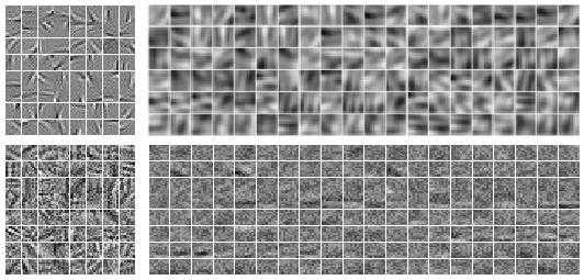
Figure 1: Top Left: first stage filters trained of a $F_{si}$ encoder trained with discriminative predictive sparse decomposition, using FISTA. Top Right: second stage filters trained the same way. Bottom Left: first layer filters in a randomly initialized network trained supervised with with an L1 penalty on the output states. Bottom Right: second stage filters trained the same way. Although the supervised filters are noisier, it is clear they learn structure similar to the unsupervised filters.

For preprocessing, the images were converted to grayscale and downsampled to $151\times 151$, then contrast-normalized with a local $9\times 9$ Gaussian-weighted neighborhood to remove the local mean and scale the neighborhood to unit std producing $143\times 143$ input images.

6.1 Architecture

Stage One: The first stage consist of an $F_{\tanh}$ or $F_{si}$ encoder module with 64 filters of size $9\times 9$ followed by a rectification module ($R_{abs}$, local mean removal and contrast normalization module ($N$), and average pooling module $P_{A}$ with $10\times 10$ pooling window and $5\times 5$ downsampling. The output of this stage consists of $64$ feature maps of size $26\times 26$. This output is used as the input to the second stage.

SIFT-SparseCoding-Pooling-SVM		$\%$
Lazebnik etal  [11]		$64.6\pm.08$
Yang etal  [26]		$73.2\pm 0.5$
Boureau etal  [3]		$75.7\pm 1.1$
ConvNets variants (learned features)		$\%$
Jarrett etal  [7]		$65.6\pm 1.0$
Kavukcuoglu etal  [9]		$66.3\pm 1.5$
Lee etal [14]		$65.4\pm 0.5$
Zeiler etal  [28]		$66.9\pm 1.1$
Ahmed etal  [1]		$67.2\pm 1.0$
Architecture	Protocol	$\%$
(1) $F_{\tanh}-R_{abs}-N-P_{A}^{pyr}$	$\mathbf{R^{+}R^{+}}$	$65.4\pm 1.0$
(2) $F_{\tanh}-R_{abs}-N-P_{A}^{pyr}$	$\mathbf{R^{+}_{L1}R^{+}_{L1}}$	$\textbf{69.0}\pm\textbf{0.2}$
(3) $F_{\tanh}-R_{abs}-N-P_{A}^{pyr}$	$\mathbf{U^{+}U^{+}}$	$66.2\pm 1.0$
(4) $F_{si}-R_{abs}-N-P_{A}$	$\mathbf{R^{+}R^{+}}$	$63.3\pm 1.0$
(5) $F_{si}-R_{abs}-N-P_{A}$	$\mathbf{R^{+}_{L1}R^{+}_{L1}}$	$64.3\pm 1.0$
(6) $F_{si}-R_{abs}-N-P_{A}$	$\mathbf{UU}$	$60.4\pm 0.6$
(7) $F_{si}-R_{abs}-N-P_{A}$	$\mathbf{U^{+}U^{+}}$	$66.4\pm 0.5$
(8) $F_{si}-R_{abs}-N-P_{A}^{pyr}$	$\mathbf{U^{+}U^{+}}$	$67.8\pm 0.4$
(9) $F_{si}-R_{abs}-N-P_{A}$	$\mathbf{DD}$	$66.0\pm 0.3$
(10) $F_{si}-R_{abs}-N-P_{A}$	$\mathbf{D^{+}D^{+}}$	$68.7\pm 0.2$
(11) $F_{si}-R_{abs}-N-P_{A}^{pyr}$	$\mathbf{D^{+}D^{+}}$	$\textbf{70.6}\pm\textbf{0.3}$

Table 1: Recognition accuracy on the Caltech-101 dataset using various architectures and training protocols. $F_{tanh}$ indicates an encoder with a $\tanh$ non-linearity followed by a gain matrix, while $F_{si}$ indicates a soft-shrink non-linearity followed by a trained lateral inhibition matrix $S$. Pyramid average pooling at the penultimate layer is denoted by $P_{A}^{pyr}$. $R$ indicates randomly initialized filters, $R_{L1}$ is random initialization with the additional L1 penalty, $U$ unsupervised pre-training, and $D$ pre-training with a discriminative term. Superscript “+” indicates global supervised fine-tuning.

Stage Two: The second stage is composed of a $F_{\tanh}$ or $F_{si}$ encoder module with 256 output feature maps, each of which combines a randomly-picked subset of 16 feature maps from the first stage using $9\times 9$ kernels. The total number of convolution kernels is $256\times 16=4096$. The size of the feature maps (before pooling) is $18\times 18$. Two types of pooling modules were used: average pooling, and pyramid average pooling. The average pooling used $6\times 6$ with $4\times 4$ downsampling, producing 256 feature maps of size $4\times 4$.

The pyramid average pooling uses multiple pooling window sizes and downsampling ratios. In addition to the 256x4x4 feature maps produced by 6x6 and 4x4 downsampling mentioned above, we added 256x3x3 feature maps produced by 8x8 pooling with 5x5 downsampling, 256x2x2 feature maps produced by 10x10 pooling with 8x8 downsampling, and 256x1x1 feature maps produced by 18x18 pooling. The results of the various pooling sizes are concatenated and fed to the classifier at the next layer.

Classifier Stage: The Stage 2 output (a single set of 256 feature maps, or multiple sets in the case of pyramid pooling) is fed to a classifier stage, which consists in an L1-L2-regularized multinomial logistic regression classifier trained with the cross-entropy loss using stochastic gradient descent. The hyperparameters for the unsupervised and supervised phases of training were selected by cross validation.

6.2 Results

Table 1 summarizes the results for various architectures and training protocols. We also include other published results for comparison. The methods listed use a framework similar to the one presented here. All results are reported as the average accuracy over 5 random splits of the dataset, each with 30 training samples per category. The training protocols are denoted by one letter for single-stage systems and two letters for two-stage systems. The letter $R$ denotes random filters, $U$ denotes unsupervised pre-training, and $D$ pre-training with a discriminative term. Superscript $+$ indicates global training using supervised gradient-descent. Comparisons between the various architectures and training protocols are discussed below. The use of max pooling instead of average pooling was attempted, but resulted in a slight decrease in accuracy of $(\approx 1\%)$.

1. Experiments (8) and (11) show that including the discriminative term in the unsupervised pre-training increases the performance by $\approx 3\%$. Our best method reaches $70.6\%$, which compares favorably with other methods in which the entire feature hierarchy is trained. Methods with better accuracy [26, 3] use SIFT at the first stage and use sparse coding with a large code size at the second stage.

2. Surprisingly, sparse-state supervised training with random initialization achieves $69\%$ with the simpler, $F_{\tanh}$ encoder. This is $1.7\%$ off of our best method with considerably less computation. This method is significantly simpler than every method that outperforms it and only requires a single stage of training. The poor performance, $64.3\%$, while using the $F_{si}$ encoder is likely due to convergence issues with the random initialization of this encoder.

3. Comparing network $(9,6)$ shows that in the absence of supervised fine-tuning, including the discriminative term increases the performance of the network by $6\%$.

4. It is clear from comparing (9,7) that including a discriminative term, either during the unsupervised phase or after (as fine-tuning), results in the same performance. The advantage of including the term in the unsupervised phase is that we can fold all the learning into a single phase, as opposed to two separate phases.

5. Comparing (9,10) shows that even though we have the discriminative term in the unsupervised phase, adding fine-tuning still increases the performance. This is because we have global training with a hierarchical system so that the second layer is able to effect the output feature maps of the first layer. This creates room for improvement which here is $2.7\%$.

6. A comparison of networks $(7,8)$ and $(10,11)$, shows that the pyramid method does increase the performance. For the full network with the discriminative term the increase is nearly $2\%$.

7 Experiments with CIfAR-10

The CIfAR-10 dataset  [10] is a hand-labeled subset of a larger dataset of 80 million $32\times 32$ color images from the web. There are $50,000$ images, $5,000$ per class, with $1,000$ images per class set aside for testing. The low resolution and high level of variability make this a challenging dataset for most recognition systems.

We use the following protocol: The data is composed of $32\times 32$ RGB color images. For preprocessing, the images were converted to YUV (luminance-chrominance). The Y (luminance) channel was locally normalized (with an $N$ module), and the U and V chrominance channels had their global mean subtracted off, and were divided by their global standard deviations.

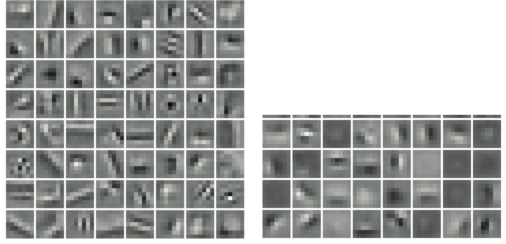
Figure 2: First stage $7\times 7$ filters learned convolutionally on $16\times 16$ color image patches (YUV encoded). The left side shows the 64 filters for the Y luminance channel. The right side shows the 32 filters for the U and V chroma channels. These chroma filters are lower frequency than the Y filters.

7.1 Architecture

Stage One: Results are reported for two separate pipelines. The only differences between the two is the pooling operator (average or max) and whether the normalization layer comes before or after the pooling layer. The best performing network uses max-pooling with an encoder $F_{si}$ trained convolutionally with $7\times 7$ kernels on $16\times 16$ image patches. There are 64 output feature maps and 96 convolution kernels. Y channel (luminance) is connected to all 64 output feature maps and each one of U and V channels is connected to randomly chosen 16 output feature maps. This is followed by an absolute value rectification, a max-pooling over $4\times 4$ windows with with a $2\times 2$ downsampling, and a local mean removal and contrast normalization with a $9\times 9$ window. The average pooling network is identical, except that order of the normalization and pooling operations is reversed. The output of this layer is $64\times 12\times 12$.

It was found empirically that average pooling produces better results when preceded by the normalization module, while max-pooling is better when followed by the normalization module. One possible explanation is that gradient-based supervised learning converges faster and to a better solution when the states of the layers have approximately zero mean and uniform variances. The contrast normalization produces zero-mean and unit variance states. The average pooling modules does not affect the mean, and scales all the variances by the pooling window size. By contrast, the max pooling shifts the means to positive values, and reduces the variances unequally. Placing the normalization module after the max pooling will restore the state to zero mean and uniform variance.

The first stage filters are shown in figure 2. The filters on the Y channel are somewhat more varied than the Caltech-101 filters, because they have been trained convolutionally. Convolutional training avoids the appearance of shifted versions of each filters, since shifted versions are already present due to the convolutions. This causes filters to be considerably more diverse, as shown by [9]. The filters to the right are from the U and V channels. The filters exhibit a clear structure, though they are considerably low frequency than the Y filters.

Stage Two: The output of the 1st stage is the input to the 2nd. The encoder uses $7\times 7$ kernels on $7\times 7$ image patches (patch-based, non-convolutional training). The second stage has 256 output feature maps, each of which combines a random subset of 32 feature maps from the previous stage for a total of 8192 convolution kernels. This is followed by an absolute value rectification, a max pooling with $3\times 3$ window without downsampling, and a local contrast normalization with a $3\times 3$ windows. The average pooling network is identical, but with the order of the normalization and pooling operations reversed. The output of this stage is $256\times 4\times 4$. The hyperparameters for the supervised and unsupervised training were selected by cross validation.

7.2 Results

Method		$\%$
$10000$ linear combinations [24]		$36.0\%$
$10$k GRBM, 1 layer with fine-tuning [10]		$64.8\%$
mcRBM-DBN(11025-8192-8192) [24]		$71.0\%$
PCA(512)-iLCC(4096)-SVM [27]		$\textbf{74.5}\%$
Architecture	Protocol	$\%$
(1) $F_{si}-R_{abs}-P_{M}-N$	$\mathbf{RR}$	$47.5\%$
(2) $F_{tanh}-R_{abs}-P_{M}-N$	$\mathbf{R^{+}R^{+}}$	$70.0\%$
(3) $F_{si}-R_{abs}-P_{M}-N$	$\mathbf{R^{+}R^{+}}$	$70.5\%$
(4) $F_{tanh}-R_{abs}-P_{M}-N$	$\mathbf{R^{+}_{L1}R^{+}_{L1}}$	73.1%
(5) $F_{si}-R_{abs}-P_{M}-N$	$\mathbf{D_{c}^{+}}$	$59.6\%$
(6) $F_{si}-R_{abs}-N-P_{A}$	$\mathbf{D_{c}^{+}}$	$60.0\%$
(7) $F_{tanh}-R_{abs}-P_{M}-N$	$\mathbf{U_{c}^{+}U^{+}}$	$74.7\%$
(8) $F_{si}-R_{abs}-P_{M}-N$	$\mathbf{U_{c}^{+}U^{+}}$	$74.8\%$
(9) $F_{si}-R_{abs}-P_{M}-N$	$\mathbf{D^{+}D^{+}}$	$74.4\%$
(10) $F_{si}-R_{abs}-N-P_{A}$	$\mathbf{D_{c}^{+}D^{+}}$	$75.0\%$
(11) $F_{si}-R_{abs}-P_{M}-N$	$\mathbf{D_{c}^{+}D^{+}}$	77.6%

Table 2: Recognition accuracy on the CIfAR-10 dataset for different architectures, and training procedures. Notations are as in Table 1. Subscript $c$ indicates convolutional pre-training (as opposed to patch-based).

Table 2 shows our method with the current state of the art in the published literature. The effects of various components is broken down in the points below. First of all, our best method yields $77.6\%$ correct recognition, which is the best ever reported in the peer-reviewed literature

1. Lines (8) and (11) show that including the discriminative term increases the performance by about $3\%$. This is similar to the increase seen with Caltech-101. Unsupervised pre-training makes a 4% difference over random initialization and purely supervised training, with convolutional, or non-convolutional discriminative. But the jump is 7% when the pre-training is both convolutional and discriminative.

2. Comparing (4,9) we again see that sparse state supervised training is competitive with patch based discriminative pre-training. The difference grows when convolutional training is used at the first stage (11). We note that this increase in performance from patch to convolutional training was not seen with training Caltech 101.

3. There is a considerable jump of nearly $3\%$ (lines (9) and (11)) obtained from convolutional training. It seems that because the internal feature representation in this CIfAR network has lower dimension (lower spatial resolution), the redundancy reduction afforded by the convolutional training makes a significant difference.

4. Consistent with the findings of [3], comparing (10) and (11) shows that max pooling outperforms average pooling by $2.6\%$. It is surprising that we have not seen this effect with Caltech. Perhaps the high level of variation in Cifar is the reason that max pooling outperforms average on this dataset. It may also be that blurring the feature maps when they are already at such a low resolution removes information necessary to learn good features.

8 Effects of Contrast Normalization

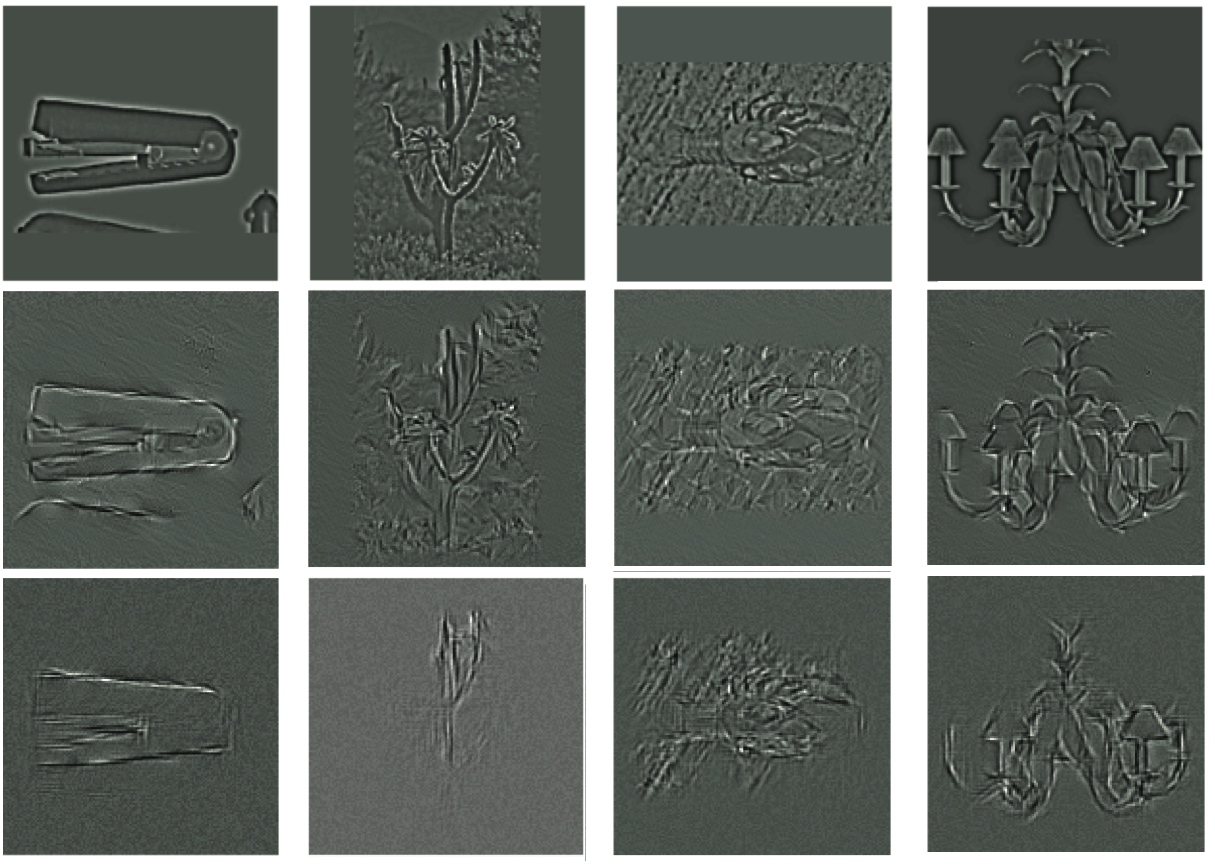
Figure 3: Hallucinated images that produce a given feature representation. Images from the Caltech-101 dataset (shown on the top row) were ran through a two-stage trained ConvNet. The output feature maps were recorded. Hallucinated inputs (middle and bottom rows) were produced by performing steepest descent in input space from a random initial condition so as to produce the same feature maps as the original images. The middle row shows reconstructions for a network with contrast normalization modules ($N$) at both stages, and the bottom row for a network without contrast normalization.

This section looks at the impact of including the local contrast normalization nonlinearity (CN) in the feature extraction process. CN has been applied to areas as diverse as sensory processing [6, 25], image denoising [22], and redundancy reduction [15] to name a few. It is also known to improve performance in higher level tasks such as object recognition [7], though the reasons for this are poorly understood.

The networks described in this section are the same as those used in the Caltech 101 experiments with 3 important differences: 1) the second layer is 128 instead of 256; 2) the number of connections between the two layers is 32 instead of 16; 3) the pooling and downsampling ratios are decreased.

The first layer has 64 $9\times 9$ convolution kernels followed by an absolute value rectification, local CN (or not), and $5\times 5$ pooling window with a $2\times 2$ downsampling step size. The results in feature maps that are $64\times 66\times 66$. These feature maps are the input to the second layer. The second layer has 128 output feature maps that combine a random subset of 32 feature maps from the first layer using $9\times 9$ kernels. This is followed by an absolute value rectification, local CN (or not), and a $4\times 4$ pooling window with a $2\times 2$ downsampling step size. This results in output feature maps that are $128\times 28\times 28$.

The experiments are done on entire images from Caltech 101. First an image is projected through the 2 layer network to produce a set of feature maps that represent the input in feature space. These feature maps are fixed and the input image is randomized. Steepest descent optimization is then used to find the optimal input for that particular set of feature maps. This process is carried out with and without CN.

The results for four different images randomly drawn from Caltech 101 are shown in figure 3. The top row is the original image which has been preprocessed. The center row is the optimal input found when CN is included. The bottom row is the optimal input found without CN. It is clear that the images synthesized using CN are are more similar to the original input images.

Network	Protocol	Accuracy $\%$
$F_{si}-R_{abs}-N-P_{A}$	$\mathbf{DD}$	$64.1\%$
$F_{si}-R_{abs}-P_{A}$	$\mathbf{DD}$	$59\%$

Table 3: The recognition accuracy for the networks used to synthesize the hallucinated images in figures 3.

This suggests that one way CN improves recognition performance is by preserving more information about the input in the feature maps. These richer feature maps provide the classifier with important characteristics of the object class that help to increase discriminability. Table 3 shows the performance of the networks on Caltech 101 $(UU)$. The increase in the networks ability to accurately synthesize the input image is correlated with an increase in its performance on the recognition task.

9 Discussion

This paper presents a thorough exploration of various training procedures for sparse, convolutional feature hierarchies. In our analysis, we introduce 1) a new unsupervised learning algorithm (DPSD) that includes a discriminative term in the sparse coding objective function, 2) a new single phase supervised training procedure that produces results similar to two-phase training methods, 3) a new multiresolution pooling mechanism that reliably increases recognition performance over traditional pooling, and 4) a new nonlinear feedforward encoder that can be trained to approximately predict the optimal sparse codes by using a smooth shrinkage nonlinearity and a cross-inhibition matrix. Additionally, we have shown that convolutional training of this architecture also improves performance. We tested this system on Caltech-101 and CIfAR-10, producing state of the art or comparable results on both datasets. The surprising result is that discriminative unsupervised pre-training with a complex encoder works well, but pure supervised with sparsity is almost as good and much simpler. We feel that these results make the use of complex multi-stage pre-training procedures unnecessary unless convolutional learning proves helpful. Finally we provided evidence indicating that contrast normalization improves recognition performance by preserving more information about the input necessary for discrimination in the feature maps.

References

- [1] A. Ahmed, K. Yu, W. Xu, Y. Gong, and E. Xing. Training hierarchical feed-forward visual recognition models using transfer learning from pseudo tasks. In ECCV, 2008.
- [2] A. Beck and M. Teboulle. A fast iterative shrinkage thresholding algorithm with application to wavelet-based image deblurring. In ISCASSP, 2009.
- [3] Y. Boureau, F. Bach, Y. LeCun, and J. Ponce. Learning mid-level features for recognition. In CVPR, 2010.
- [4] I. Daubechies, M. Defrise, and C. De Mol. An iterative thresholding algorithm for linear inverse problems with a sparsity constraint. Comm. Pure Appl. Math, 2004.
- [5] K. Gregor and Y. LeCun. Learning fast approximations of sparse coding. In ICML, 2010.
- [6] D. J. Heeger. Normalization of cell responses is cat striate cortex. Visual Neuroscience, 9:181–197, 1992.
- [7] K. Jarrett, K. Kavukcuoglu, M. Ranzato, and Y. LeCun. What is the best multi-stage architecture for object recognition? In ICCV, 2009.
- [8] K. Kavukcuoglu, M. Ranzato, and Y. LeCun. Fast Inference in Sparse Coding Algorithms with Applications to Object Recognition. http://arxiv.org/abs/1010.3467v1, 2010.
- [9] K. Kavukcuoglu, P. Sermanet, Y. Boureau, K. Gregor, M. Mathieu, and Y. LeCun. Learning convolutional features hiearchies for visual recognition. In NIPS, 2010.
- [10] A. Krizhevsky. Learning mutliple layers of features from tiny images. Master’s thesis, Dept of Computer Science, University of Toronto, 2009.
- [11] S. Lazebnik, C. Schmid, and J. Ponce. Beyond bags of features: Spatial pyramid matching for recognizing natural scene categories. In CVPR, June 2006.
- [12] Y. LeCun, L. Bottou, Y. Bengio, and P. Haffner. Gradient-based learning applied to document recognition. Proceedings of the IEEE, 86(11):2278–2324, November 1998.
- [13] H. Lee, E. Chaitanya, and A. Y. Ng. Sparse deep belief net model for visual area v2. In NIPS, 2007.
- [14] H. Lee, R. Grosse, R. Ranganath, and A. Y. Ng. Convolutional deep belief networks for scalable unsupervised learning of hierarchical representations. In Proc. ICML, 2009.
- [15] S. Lyu and E. Simoncelli. Nonlinear image representation using divisive normalization. In CVPR, 2008.
- [16] J. Mairal, F. Bach, J. Ponce, and G. Sapiro. Online learning for matrix factorization and sparse coding. Journal of Machine Learning Research, 11:19–60, 2010.
- [17] J. Mairal, F. Bach, J. Ponce, G. Sapiro, and A. Zisserman. Discriminative learned dictionaries for local image analysis. In CVPR, 2008.
- [18] J. Mairal, F. Bach, J. Ponce, G. Sapiro, and A. Zisserman. Supervised Dictionary Learning. NIPS, 21, 2009.
- [19] J. Mairal, F. Bach, and G. Sapiro. Sparse representation for image restoration. In IEEE Transactions of Image Processing, volume 17, pages 53–69, January 2008.
- [20] S. Mallat and Z. Zhang. Matching pursuits with time-frequency dictionaries. IEEE Transactions on Signal Processing, 41(12):3397:3415, 1993.
- [21] B. A. Olshausen and D. J. Field. Sparse coding with an overcomplete basis set: a strategy employed by v1? Vision Research, 37:3311–3325, 1997.
- [22] J. Portilla, V. Strela, M. Wainwright, and E. Simoncelli. Image denoising using scale mixtures of gaussians in the wavelet domain. IEEE Trans. Image Processing, 12(11):1338–1351, 2003.
- [23] M. Ranzato, Y. Boureau, and Y. LeCun. Sparse feature learning for deep belief networks. In NIPS, 2007.
- [24] M. Ranzato and G. E. Hinton. Modeling pixel means and covariances using factorized third order boltzmann machines. In CVPR, 2010.
- [25] E. Simoncelli and D. J. Heeger. A model of neuronal responses in visual area mt. Vision Research, 38:743–761, 1998.
- [26] J. Yang, K. Yu, Y. Gong, and T. Huang. Linear spatial pyramid matching using sparse coding for image classification. In CVPR, 2009.
- [27] K. Yu and T. Zhang. Improved local coordinate coding using local tangents. ICML, 2010.
- [28] M. Zeiler, D. Krishnan, G. Taylor, and R. Fergus. Deconvolutional networks. In CVPR. CVPR, 2010.