Lagrangian Relations and Linear billiards

Abstract.

Motivated by the high-energy limit of the $N$-body problem we construct non-deterministic billiard process. The billiard table is the complement of a finite collection of linear subspaces within a Euclidean vector space. A trajectory is a constant speed polygonal curve with vertices on the subspaces and change of direction upon hitting a subspace governed by “conservation of momentum” (mirror reflection). The itinerary of a trajectory is the list of subspaces it hits, in order. (A) Are itineraries finite? (B) What is the structure of the space of all trajectories having a fixed itinerary? In a beautiful series of papers Burago-Ferleger-Kononenko [BFK] answered (A) affirmatively by using non-smooth metric geometry ideas and the notion of a Hadamard space. We answer (B) by proving that this space of trajectories is diffeomorphic to a Lagrangian relation on the space of lines in the Euclidean space. Our methods combine those of BFK with the notion of a generating family for a Lagrangian relation.

1. Introduction.

.

1.1. Euclidean Data. Point Billiards. Motivating Example.

Consider a Euclidean vector space $E$ endowed with a finite collection ${\mathcal{L}}$ of linear subspaces which we call “collision subspaces”. Write

(1) $$C=\bigcup_{L\in{\mathcal{L}}}L\qquad\text{ (collision locus)}$$

for the collision locus and

(2) $$E^{0}=E\setminus C\qquad\text{ (our billiard table)}$$

for its complement. Play billiards on $E^{0}$ !

A “billiard trajectory” will be a certain type of polygonal curve $q:\mathbb{R}\to\mathbb{E}$ all of whose vertices are collisions, i.e. lie on $C$. When $q$ hits a subspace $L\in{\mathcal{L}}$ it switches directions by bouncing off of $L$ according to the laws of reflection (see equations (4), (5) below). Imagine light rays bouncing off of a finite collection of reflective wires (lines) in $E=\mathbb{R}^{3}$.

1.1.1. Motivating Example: $N$-body billiards

$E=(\mathbb{R}^{d})^{N}$ is the configuration space for the $N$ massive point particles moving in $d$–dimensional Euclidean space $\mathbb{R}^{d}$. Endow $E$ with its mass metric, by which we mean the inner product whose squared norm is twice the kinetic energy. Take ${\mathcal{L}}$ to consist of the $N\choose 2$ binary collision subspaces

(3) $$\Delta_{ab}=\{q=(q_{1},\ldots,q_{N}),q_{i}\in\mathbb{R}^{d}:q_{a}=q_{b}\}\subset E\quad\mbox{ for some pair }a\neq b.$$

We call this class of examples “$N$-body billiards”. See the next section for details.

1.1.2. Billiard Rules.

We now define what it means for a polygonal curve $q:\mathbb{R}\to E$ to be a billiard trajectory. By a collision point for $q$ we mean a time $t$ or the corresponding point $q(t)$ such that $q(t)\in C$. Thus at a collision point $q(t)\in L$ for some $L\in{\mathcal{L}}$. We assume that collision points are discrete. In particular no edge of $q$ lies within an $L$. Every vertex of $q$ is a collision point. The velocities $v_{-},v_{+}$ of $q$ immediately before and after collision with $L\in{\mathcal{L}}$ are well-defined and locally constant. They suffer a jump $v_{-}\mapsto v_{+}$ at collision. Let

$$\pi_{L}:E\to L$$

be orthogonal projection onto $L$. We require each velocity jump to obey the rules:

(4) $$\|v_{-}\|=\|v_{+}\|\qquad\text{ ``conservation of energy''}$$

(5) $$\pi_{L}(v_{+})=\pi_{L}(v_{-})\qquad\text{ ``conservation of momentum''}$$

In N-body billiards (1.1.1) these rules correspond to conservation of energy and momentum. (Note that the rules allow for no jump: $v_{-}=v_{+}$.)

To summarize, a billiard trajectory for $(E,\langle\cdot,\cdot\rangle,{\mathcal{L}})$ is an oriented polygonal curve in $E$ with vertices on collision subspaces, and no edge of which lies within a collision subspace. At each collision the velocity jump $v_{-}\to v_{+}$ obeys the two rules (4, 5) above. Without loss of generality we will assume the curve’s speed is $1$.

1.1.3. Multiple collisions.

The attentive reader will have noticed that the law of reflection (5) is ambiguous if the collision point $q_{*}$ belongs to more than one $L$. This ambiguity is analogous to the problem of trying to define standard billiard dynamics at the corner pocket of a polygonal billiard table in the plane. We get around this ambiguity by agreeing to choose one of the collision subspaces to which $q_{*}$ belongs and then using only that subspace in implementing law (5). Thus we view billiard trajectories with multiple collisions as coming with the extra structure of a labelling of collision points, with each collision point being labelled by one of the $L\in{\mathcal{L}}$ to which it belongs. For more on problems arising with multiple collisions see subsection 2.1 further on.

1.1.4. Dimension and Transversality.

For simplicity of exposition we will henceforth assume that each subspace $L$ has the same codimension $d$ and $d\geq 1$. This assumption excludes various pathologies such as $L_{1}\subset L_{2}$ occuring within our collection ${\mathcal{L}}$ of subspaces.

In addition to being all of the same codimension $d$, the collection (eq (3)) of collision subspaces for N-body billiards are pairwise transversal: ${\rm codim}(L_{1}\cap L_{2})=2d$ for all distinct pairs $L_{1},L_{2}\in{\mathcal{L}}$. We believe such transversality assumptions may be very useful in future work.

1.1.5. Non-deterministic Dynamics.

For a given incoming $v_{-}\in E\setminus 0$ to a $q_{*}\in L$ there is a $(d-1)$–dimensional sphere’s worth of choices for the outgoing $v_{+}$’s, namely the set of all solutions to eq (4, 5) for that fixed $v_{-}$. It follows that the billiard process is non-deterministic: there is no univalued rule that takes us from the past motion to the future motion. However, we do not view our billiard dynamics as a stochastic process. Rather we think of our billiard trajectories as arising as limits of deterministic $N$-body dynamics, and we are interested in what is the set of all possible limits. See section 2 below.

(Even if $d=1$ we do not have deterministic dynamics, since the $0$-sphere consists of two choices. It is standard to turn this case into a deterministic dynamics by requiring transversality: $v_{+}\neq v_{-}$ at each collision. This is what is done for $N$ point particles moving on the line: the dynamics preserves their order on the line. The game is equivalent to playing billiards on a closed polyhedral cone in $\mathbb{R}^{N}$.)

1.2. Basic Questions and Main result.

1.2.1. Fundamental Finiteness Theorem.

QUESTION 1. Is the total number of collisions of a billiard trajectory finite?

The answer is the fundamental theorem of the subject.

Background Theorem 1 ([BFK1, BFK2]).

There is a $K=K(E,\langle\cdot,\cdot\rangle,{\mathcal{L}})$ such that every trajectory has less than or equal to $K$ collisions.

To appreciate the subtlety of the problem of computing the smallest $K$, even in apparently simple deterministic ($d=1$) situations, we strongly urge the reader to take a peek at [Gal].

1.2.2. Itineraries.

Definition 1.

The itinerary of a billiard trajectory is the list of collision subspaces $L\in{\mathcal{L}}$ that it intersects, in their order of occurrence.

By the Background Theorem of BFK just stated, any realized itinerary has length less than or equal to $K$. So if there are a total of $M$ subspaces in ${\mathcal{L}}$, then the set of all realized itineraries is a finite set of length less than $M^{K}$. (Repeats such as $L_{1}L_{1}\ldots$ are not allowed, hence the strict inequality.)

QUESTION 2. What is the finite set of all itineraries which are realized by some billiard trajectory?

This is a hard question about which we have very little to say.

We can observe that beyond $L_{i+1}\neq L_{i}$ there may be other ‘topological’ restrictions on the allowable itineraries. For example, for $N\geq 4$ bodies on the line ($d=1$; $E=\mathbb{R}^{N}$) after the itinerary $(\Delta_{12},\Delta_{34},\Delta_{23})$ particles 1 and 4 can no longer be neighbors, whether or not collisions change the ordering (are transverse). So $(\Delta_{12},\Delta_{34},\Delta_{23},\Delta_{14})$ cannot be realized.

In section 8.1 we give some partial results regarding this question when each $L$ is a line.

1.2.3. Space of trajectories realizing a given itinerary

Suppose a particular itinerary is realized. We can then ask about all of its realizations.

QUESTION 3. What is the structure (dimension, smoothness, symplectic character) of the space of all billiard trajectories having a given itinerary?

Answering Question 3 is the point of our paper. From now on we fix an itinerary $L_{1}L_{2}\ldots L_{k}$, with $L_{i}\in{\mathcal{L}}$.

Defining the space ${\mathcal{B}}$ of point billiard trajectories realizing the itinerary. Write ${\mathcal{B}}(L_{1}\ldots L_{k})$, or simply ${\mathcal{B}}$ for the space of all billiard trajectories realizing the given itinerary. Let us be more precise: a billiard trajectory $q$ is in the subset ${\mathcal{B}}(L_{1}\ldots L_{k})$ if and only if there are exactly $k$ distinct collision times:

(6) $$t_{1}<t_{2}<\ldots t_{k},\qquad q(t_{i}):=q_{i}\in L_{i}.$$

We emphasize that

(7) $$q_{i}\neq q_{i+1},\qquad i=1,2,\ldots,k-1$$

since $|q_{i+1}-q_{i}|=t_{i+1}-t_{i}>0$. Also $q_{i+1}-q_{i},q_{i}-q_{i-1}\notin L_{i}$ since no edge of $q$ lies in the collision locus. Condition (7) does not exclude the possibility of $q_{i}\in L^{\prime}$ for some $L^{\prime}\in{\mathcal{L}}$, $L^{\prime}\neq L_{i},L_{i+1},L_{i-1}$. In this case we label $q_{i}$ with $L=L_{i}$ when applying our ‘conservation of momentum” rule eq (5). We endow ${\mathcal{B}}$ with the compact-open topology.

A trajectory $q\in{\mathcal{B}}(L_{1}\ldots L_{k})$ has an initial ray $r_{-}$ parameterized by the initial segment $(-\infty,t_{1})$ where $q_{1}=q(t_{1})$ is the first collision. Similarly $q$ has a final ray $r_{+}$ parameterized by the final segment $(t_{k},\infty)$ where $q_{k}=q(t_{k})$ is the final collision along $q$. Extend the rays to oriented lines $\ell_{-},\ell_{+}$. We want to think of the fixing of the itinerary as defining a “scattering map”

(8) $$\ell_{+}\mapsto\ell_{+}$$

on the space ${\rm\it LINES}(E)$ of oriented lines in $E$. (We will elucidate the structure of ${\rm\it LINES}(E)$ as a symplectic manifold momentarily.) However, this “scattering map” is almost never a map in that one $\ell_{-}$ may give rise to many $\ell_{+}$’s. See example 1 below. Instead we have “scattering relation”

$${\mathcal{R}}={\mathcal{R}}(L_{1}\ldots L_{k})\subset{\rm\it LINES}(E)\times{\rm\it LINES}(E).$$

Definition 2.

The scattering relation ${\mathcal{R}}={\mathcal{R}}(L_{1}L_{2}\ldots L_{k})$ associated to the chosen itinerary $L_{1}L_{2}\ldots L_{k}$ consists of all pairs $(\ell_{-},\ell_{+})$ of incoming and outgoing lines for billiard trajectories $q\in{\mathcal{B}}(L_{1}\ldots L_{k})$.

We have just defined a continuous map

$${\mathcal{B}}\to{\mathcal{R}}\subset{\rm\it LINES}(E)\times{\rm\it LINES}(E)$$

which sends each trajectory $q\in{\mathcal{B}}(L_{1}\ldots L_{k})$ to its incoming and outgoing (oriented) lines. The image of this map is the scattering relation. The group of time translations acts on the space of billiard trajectories, sending $q(t)$ to $q(t-t_{0})$, for $t_{0}\in\mathbb{R}$, without altering the itinerary or the incoming or outgoing line. Thus our map into the scattering relation induces a map on the quotient domain with the same image. We name this map the scattering projection.

(9) $${\rm\it SCAT}:{\mathcal{B}}/\mathbb{R}\longrightarrow{\mathcal{R}}\subset{\rm\it LINES}(E)\times{\rm\it LINES}(E)$$

We can now state our main result.

Theorem 1.

The scattering relation ${\mathcal{R}}$ is a Lagrangian relation on the symplectic manifold ${\rm\it LINES}(E)$ of oriented lines in $E$. In particular ${\mathcal{R}}$ is a smooth manifold of dimension $2(\dim(E)-1)$. The scattering projection (eq (9)) defines a diffeomorphism between ${\mathcal{B}}/\mathbb{R}$ and ${\mathcal{R}}$. In particular, modulo time translation, a point billiard trajectory realizing the given itinerary is uniquely determined by its incoming and outgoing lines.

For completeness, we recall for the reader the definition of “Lagrangian relation” and the symplectic structure on ${\rm\it LINES}(E)$ in what immediately follows.

1.2.4. Lagrangian relations

Definition 3.

A Lagrangian relation on a symplectic manifold $(P,\omega)$ is a Lagrangian submanifold ${\mathcal{R}}$ of the product symplectic manifold $\bar{P}\times P$, where the bar of “$\bar{P}$” means we endow the product with the symplectic structure $-\omega\oplus\omega$.

Graphs of symplectic maps $P\to P$ are Lagrangian relations. We think of Lagrangian relations as generalized symplectic maps, that is, symplectic maps which are “allowed to go vertical” at various places.

1.2.5. The symplectic structure on the space of lines.

An oriented line $\ell\in{\rm\it LINES}(E)$ can be represented by an initial position $A\in E$ and an initial velocity $v_{A}\in E_{v}\cong E$. (We use the subscript $v$ in “$E_{v}$” to keep track of who is a velocity and who is a position.) The line associated to $(A,v_{A})$ is parameterized as $A+tv_{A}$. We will insist that velocities $v_{A}$ are unit: $|v_{A}|=1$. $(A,v_{A})$ and $(C,v_{C})$ represent the same oriented line if and only if $v_{A}=v_{C}$ and $C=A+sv_{A}$ for some real number $s$. There is a unique point $Q\in\ell$ closest to the origin of $E$. This $Q$ is determined by the algebraic condition $\langle Q,v_{A}\rangle=0$. Choosing $Q$ as the initial position $A$ on $\ell$ sets up a diffeomorphism between the space ${\rm\it LINES}(E)$ of oriented lines in $E$ and the tangent bundle of the unit sphere in $E$:

$${\rm\it LINES}(E)\cong TS(E_{v})=\{(v,Q)\in E_{v}\times E:|v|=1,Q\perp v\}.$$

Use the Euclidean structure to identify $TS(E_{v})$ with $T^{*}S(E_{v})$, thereby giving the space of lines a symplectic structure.

Remark. The diffeomorphism ${\rm\it LINES}(E)\to TS(E_{v})$ reverses the role of positions and velocities. The position $v\in S(E_{v})$ at which the tangent vector $(v,Q)$ is attached represents the velocity vector $v=v_{A}$ of the corresponding line, while the tangent or $Q$-part of $(v,Q)$ represents an initial position point on the line $\ell$, namely the closest point to $0$.

1.2.6. Lines as a reduced space

The space of oriented lines can be recast as a symplectic reduced space. Let $H(A,v)=\frac{1}{2}|v|^{2}$ be the usual Hamiltonian for free particle motion. Here $(A,v)\in E\times E_{v}\cong E\times E^{*}\cong T^{*}E$. The flow of the Hamiltonian vector field for $H$ is $\phi_{t}(A,v_{A})=(A+tv_{A},v_{A})$ which is a symplectic $\mathbb{R}$ action on the full phase space. Its integral curves are lines. The level set $H^{-1}(1/2)$ consists of those initial conditions $(A,v)$ such that $|v|=1$. The space ${\rm\it LINES}(E)$ of oriented lines is thus the sub-quotient $H^{-1}(1/2)/\mathbb{R}$ of $E\times E_{v}$ by this $\mathbb{R}$ action. This sub-quotient construction is precisely the symplectic reduction construction: ${\rm\it LINES}(E)$ with its symplectic structure is an instance of the construction of the “symplectic reduced space”. Write

(10) $$\pi:E\times S(E_{v})\to{\rm\it LINES}(E)$$

for the corresponding quotient map. Thus $\pi(A,v)=\pi(\tilde{A},\tilde{v})$ if and only if $\tilde{v}=v$ and $\tilde{A}=A+tv$ for some $t\in\mathbb{R}$.

1.2.7. The unreduced scattering relation

In order to prove and to better understand our main theorem 1 we must “unreduce” the relation ${\mathcal{R}}$ by working directly with normalized initial conditions $(A,v_{A})\in E\times S(E_{v})$ instead of the associated oriented line $\pi(A,v)=\ell$. If $q(t)$ is a billiard trajectory in ${\mathcal{B}}(L_{1}\ldots L_{k})$ consider again its initial ray $r_{-}\subset\ell_{-}$ and final ray $r_{+}\subset\ell_{+}$. Pick corresponding points $A\in r_{-}$, $B\in r_{+}$ and the corresponding directions $v_{A},v_{B}$. We emphasize that we are saying nothing about the times $t_{A},t_{B}$ at which the points $A,B$ are selected along $q(t)$. In this way we have chosen pairs $(A,v_{A}),(B,v_{B})\in E\times E_{v}$. The unreduced statement of theorem 1 is

Theorem 2.

For each $q\in{\mathcal{B}}$ consider the two-parameter family of pairs of boundary conditions

$$\big{(}(A,v_{A}),(B,v_{B})\big{)}=\big{(}(q(t_{0}),\dot{q}(t_{0})),(q(t_{k+1}),\dot{q}(t_{k+1}))\big{)}$$

lying on the incoming and outgoing rays of $q$. (Here $t_{0}<t_{1}$ and $t_{k+1}>t_{k}$ as per eq (6).) As $q$ varies over ${\mathcal{B}}$ these pairs sweep out a Lagrangian relation $\tilde{\mathcal{R}}=\tilde{\mathcal{R}}(L_{1}\ldots L_{k})$ on $E\times E_{v}$. The projection $((A,v_{A}),(B,v_{B}))\mapsto(A,B)$ maps $\tilde{\mathcal{R}}$ diffeomorphically onto an open subset of $E\times E$. The projection of $\tilde{\mathcal{R}}$ to ${\rm\it LINES}(E)\times{\rm\it LINES}(E)$ by $\pi\times\pi$ (where $\pi$ is as in eq 10) is the relation ${\mathcal{R}}$ of theorem 1.

Remark on algebraicity. Our Lagrangian relations are semi-algebraic varieties: they are defined by algebraic equations together with algebraic inequalities. This fact follows from our proof of the theorem using generating functions.

Remark: Scaling, Symmetries and Conservation Laws. Point billiard trajectories enjoy a scaling symmetry. $N$-body billiards enjoy translational and rotational symmetries and the consequent conserved quantities of linear and angular momentum. Details of these symmetries are discussed in section 7.

2. Motivation : The Gravitational $N$–Body Problem.

We go into some detail regarding our underlying motivation. The basic set-up, $E=(\mathbb{R}^{d})^{N}$ with the collision subspaces being the binary collision subspaces $\Delta_{ab}$ was described above in subsection 1.1.1 and we keep the same notation.

Positive energy solutions to the gravitational two-body problem, viewed in a center-of-mass frame, consist of a pair of coplanar hyperbolas sharing the origin as a focus. Viewed from afar away, these hyperbolas become indistinguishable from their asymptotes: the two bodies come in along their separate rays, bounce off each other, to head back to infinity along different rays.

For the gravitational $N$-body problem the same space-time picture holds when viewed from away from all close encounters. Each body moves nearly on a straight line at nearly constant speed until it comes into very close vicinity of another body at which time it veers off to recede along another near-line at near-constant speed. In the limit , what happens at these close encounters is the bodies “bounce off” each other. The direction of this “bouncing” will look random unless we know detailed specifics of the incoming motion. Without these details, all we can say is that each bounce is an elastic collision : total energy and linear momentum are conserved. These two conservation laws are encoded by our rules of reflection (eq (4, 5).

Thus we expect certain families of positive energy solutions to the graviational $N$-body problem will limit onto $N$-body billiard trajectories as described above (see subsection 1.1.1). In a subsequent paper we will prove this assertion by showing that $N$-body billiard trajectories are “shadowed” by families of trajectories of positive energy solutions to the gravitational $N$-body problem.

2.1. Multiple Collisions and clusters.

A collision between three or more particles (or two or more simultaneous binary collisions) corresponds to a point $q\in(\mathbb{R}^{d})^{N}$ lying in several $\Delta_{ab}$. The paper of Mather and McGehee [McG], and subsequent work on non-collision singularities based on their ideas make suspect the validity of our underlying assumption (4) of conservation of kinetic energy when trying to model such multiple collision events with point billiards. Mather and McGehee establish the existence of a set of initial conditions for 4 bodies (on the line) where the kinetic energy starts out $O(1)$ and in a finite time becomes arbitrarily large, arbitrarily far away from the close encounter region. The infinite negative potential energy well of near-triple collision serves as a source which one of the bodies can extract to make its speed arbitrarily high. We imagine the following caricature of celestial mechanics based on the notion of cluster decompositions [DG], where each clusters represents a subset of close tightly bound particles. Total energy and momentum is preserved for each isolated cluster. But not all energy need be kinetic. We could even allow trajectories to move inside intersections of the $\Delta_{ab}$, corresponding to systems that are bound over some large interval of time. At collisions between clusters, corresponding groups of particles can experience inelastic scattering, potential energy being stored in groups or released from it, and redistributed.

3. Generating Families and the proof.

The chord length between successive impacts of the ball with the table serves as the generating function for the standard billiard map associated to a convex table in the plane. So it is not a great surprise that the path length of finite segments of polygonal paths realizing the given itinerary serves a similar function for our non-deterministic billiard processes. Fix points $A=q_{0}$ on the incoming ray and $B=q_{k+1}$ on the outgoing ray of the billiard trajectory $q\in{\mathcal{B}}$. Let $q_{i}\in L_{i}$ be the intermediate collision points as per eq (6). Then the length of the segment $q([t_{0},t_{k+1}])$ is:

(11) $$S(A,q_{1},\ldots,q_{k},B)=|A-q_{1}|+|q_{1}-q_{2}|+\ldots+|q_{k-1}-q_{k}|+|q_{k}-B|$$

and this is also the travel time of this segment. We turn this observation around to find the billiard trajectories as critical points of $S$.

Minimization Problem.
Fix $A,B\in E\setminus C$. Minimize (11) over all intermediate choices $q_{i}\in L_{i}$.

Write $xy$ for the line segment joining $x$ to $y$, $x,y\in E$, parameterizing $xy$ so as to have unit speed. If $x_{i}\in E$ are a collection of points then by $x_{1}x_{2}x_{3}\ldots x_{n}$ we will mean the polygonal path with $n-1$ edges $x_{i}x_{i+1}$. Let

$$\Lambda=L_{1}\times L_{2}\times\ldots\times L_{k}.$$

Then if $A,B\in E$ and $\lambda=(q_{1},\ldots,q_{k})\in\Lambda$ we write $A\lambda B$ for the piecewise linear segment $Aq_{1}q_{2}\ldots q_{k}B$.

Definition 4.

We will say that $\lambda\in\Lambda$ is “generic” if $q_{1}\notin L_{2},q_{k}\notin L_{k-1}$ and $q_{i}\notin L_{i-1}\cup L_{i+1},1<i<k$.

We will say that $(A,\lambda,B)\in E\times\Lambda\times E$ is ‘generic” if $\lambda$ is generic, if $A,B\in E^{0}$ and if the rays $q_{i}A$ and $q_{k}B$ have no collisions besides their initial points $q_{1},q_{k}$.

We will call the open set of all generic points in $E\times\Lambda\times E$ the “generic set”.

Define

(12) $$S_{A,B}:\Lambda\to\mathbb{R};\quad S_{A,B}(q_{1},q_{2},\ldots,q_{k})=S(A,q_{1},q_{2},\ldots,q_{k},B)$$

by viewing the action (11) to be a function of the intermediate intersection points $q_{i}$ alone, with $A,B\in E$ as parameters.

Proposition 1.

Suppose $(A,\lambda,B)$ is generic in the sense of definition 4. Then the following are equivalent.

• (A) $\lambda$ is a critical point of $S_{A,B}$
  

• (B) $A\lambda B$ is a segment of a billiard trajectory realizing the given itinerary.

If either condition holds then the direction of the incoming line of the associated billiard trajectory is $v_{A}=-\nabla_{A}S(A,\lambda,B)$ while the direction of the outgoing line is $v_{B}=+\nabla_{B}S(A,\lambda,B)$ where $\nabla_{A}S$, $\nabla_{B}S:E^{0}\times\Lambda\times E^{0}\to E$ denote the gradients with respect to the $A,B$ variables.

Example 1.

[Total Collision] Consider the case ${\mathcal{L}}=\{0\}$, so that the only subspace is the 0 subspace. A linear billiard trajectory realizing the itinerary $(0)$ consists of an angle with vertex at $0$. The parameter space $\Lambda$ is the single point $0$. The action is $S(A,0,B)=|A|+|B|$. The intermediate collision point $q_{1}=0$ cannot be varied so the condition $d_{\lambda}S=0$ is vacuous. We compute $\nabla_{A}S=A/|A|,\nabla_{B}S=B/|B|$ consequently the Lagrangian relation of theorem 2 consists of all quadruples $((A,v_{A}),(B,v_{B}))\in TE\times TE$ for which $v_{A}=-A/|A|$ and $v_{B}=B/|B|$, and $A,B\neq 0$. The first pair $(A,-A/|A|)$ represents the initial position and velocity of a line thru the origin, moving towards the origin. The final pair $(B,B/|B|)$ represents the initial position and velocity for a line thru the origin moving away from the origin. Our incoming line and outgoing line both pass through the origin, so their “$Q$ parts” are $0$. (See subsubsection 1.2.5.) Their $v$ parts, $v_{A}$ and $v_{B}$ are arbitrary unit vectors. The Lagrangian relation ${\mathcal{R}}$ of theorem 1 is the product of the two zero sections of $T^{*}S(E)={\rm\it LINES}(E)$.

Proposition 1 asserts that $S$ is a “generating family” (also known as a “Morse family”) for the Lagrangian relation of theorem 2. We recall the notion of a generating family.

Definition 5.

The function $F:E\times\Lambda\times E\to\mathbb{R}$ is a generating family for the Lagrangian relation ${\mathcal{R}}$ on $E\times E_{v}$ if ${\mathcal{R}}$ consists of those quadruples (pairs of pairs) $\big{(}(A,v_{A}),(B,v_{B})\big{)}\in(E\times E_{v})\times(E\times E_{v})$ for which there exists a $\lambda\in\Lambda$ such that

• (i) $(A,\lambda,B)$ is a smooth point of $F$, and

• (ii) $d_{\lambda}F(A,\lambda,B)=0$, $v_{A}=-\nabla_{A}F(A,\lambda,B)$ and $v_{B}=+\nabla_{B}F(A,\lambda,B)$.

Here $\nabla_{A},\nabla_{B}$ are the gradients with respect to these first and last component variables, $A,B$ and $d_{\lambda}F(A,\lambda,B)\in\Lambda^{*}$ is the differential with respect to $\lambda$.

The notion of generating family was formalized by Hörmander in [Hor1] [Hor2, Def. 25.4.3] under the name of “phase function”. Libermann and Marle [LiMa] use the name “Morse family” and we find their treatment exceptionally clear. (See Definition 1.10 in [LiMa, Appendix 7.1].) Paraphrasing: “Let $\pi:B\to N$ be a submersion and $S:B\to{\mathbb{R}}$ be a differentiable function. The function $S$ is called a Morse family (for $N$, or for $R\subset T^{*}N$) if the image of the one-form $dS:B\to T^{*}B$ and the conormal bundle to the fibers of $\pi$, are transverse within $T^{*}B$. This transverse intersection is necessarily smooth and pushes down to $T^{*}N$ where it forms a Lagrangian submanifold $R$, the Lagrangian submanifold for which $S$ is the ‘Morse family’.”

The transversality condition in the definition just given of a Morse family is needed to insure that the corresponding Lagrangian submanifold is smooth. In our case we establish smoothness by establishing:

Proposition 2.

Every critical point $\lambda$ of $S_{AB}$ which is a generic point in the sense of definition 4 is a non-degenerate critical point, so transversality holds as discussed above. Indeed, the Hessian of $S_{A,B}$ at $\lambda$ is positive definite.

3.1. Proof of proposition 1.

For the function $x\mapsto|x|$ we have that $d|x|=\frac{\langle x,dx\rangle}{|x|}$. (The algebraic meaning of ‘$dx$’ here, as per computations found frequently in Chern or Cartan, is that $dx$ is the identity map on $E$, this being the differential of the map $x\mapsto x$. In other words, for $v\in E$ $(d|x|)(v)=\frac{\langle x,v\rangle}{|x|}$.) Similarly if $x_{0}\in E$ is a constant vector then $d|x-x_{0}|=\frac{\langle x-x_{0},dx\rangle}{|x-x_{0}|}=\langle n(x,x_{0}),dx\rangle$, where we write

$$n(x,y)=\frac{x-y}{|x-y|}$$

for the unit vector pointing from $y$ to $x$, assuming $x\neq y$. Now write $d_{i}$ for the differential of $S_{A,B}$ with respect to $q_{i}$, keeping the other $q_{j}$ constant. We have

$$d_{i}S_{A,B}=d_{i}(|q_{i-1}-q_{i}|+|q_{i}-q_{i+1}|)=\langle n(q_{i},q_{i-1}),dq_{i}\rangle+\langle n(q_{i},q_{i+1}),dq_{i}\rangle.$$

Since $n(y,x)=-n(x,y)$, this yields

$$d_{i}S_{A,B}=\big{\langle}n(q_{i},q_{i-1})-n(q_{i+1},q_{i})\ ,\ dq_{i}\big{\rangle}.$$

Now $dq_{i}$ is the identity on $L_{i}$, so this differential is zero if and only if $n(q_{i},q_{i-1})-n(q_{i+1},q_{i})\perp L_{i}$ which is the same as requiring that $\pi_{i}(n(q_{i},q_{i-1})-n(q_{i+1},q_{i}))=0$, where we have written $\pi_{i}$ for $\pi_{L_{i}}$. But if the piecewise linear trajectory $Aq_{1}q_{2}\ldots q_{k}B$ is parametrized by arc length, traveling from $A$ to $B$, then its velocity just before collision with $L_{i}$ is $v_{i,-}=n(q_{i},q_{i-1})$ and its velocity just after collision is $v_{i,+}=n(q_{i+1},q_{i})$, so that our condition of criticality is equivalent to the condition of conservation of momentum (equation (5)) at collision $i$. Finally $dS_{A,B}=0$ if and only if for $i=1,2,\ldots,k$ we have $d_{i}S_{A,B}=0$. $\Box$

We postpone the proof of proposition 2 to section 5.

3.2. Proof of (most of) theorem 2.

Let $q_{0}\in{\mathcal{B}}(L_{1}\ldots L_{k})$ with initial ray $\ell_{in,0}$ and final ray $\ell_{out,0}$. Let $\lambda_{0}=q_{1}^{0},q_{2}^{0},\ldots,q_{k}^{0}$ be its collision points. According to the definition of a billiard trajectory we cannot have $q_{i+1}\in L_{i}$, $1\leq i\leq k-1$ for otherwise segment $q_{i}q_{i+1}\subset L_{i}$ which is forbidden. Similarly $q_{i-1}\notin L_{i}$ for $2\leq i\leq k$. Choose points $A_{0}\in\ell_{in,0}$, $B_{0}\in\ell_{out,0}$. Then $A_{0},B_{0}\notin C$. Thus $(A_{0},\lambda_{0},B_{0})\in E\times\Lambda\times E$ is a generic point. And according to proposition 1, $\lambda_{0}$ is a critical point of $S_{A_{0},B_{0}}$.

Now flip the logic around. Consider the map $E\times\Lambda\times E\to\Lambda^{*}$

(13) $$(A,\lambda,B)\ \longmapsto\ dS_{A,B}(\lambda)\in\Lambda^{*}.$$

Proposition 1 asserts that the zeros $(A,\lambda,B)$ of this map which are generic points (in the sense of definition 4) are precisely the billiard segments for some $q\in{\mathcal{B}}(L_{1},L_{2},\ldots,L_{k})$.

The chosen segment of $q_{0}$ from $A_{0}$ to $B_{0}$ is such a zero. We use Proposition 2 in conjunction with the Implicit Function Theorem to get nearby, smoothly varying, zeros. The derivative of map (13) with respect to $\lambda\in\Lambda$ at $A_{0}\lambda_{0}B_{0}$ is the Hessian of $S_{A_{0},B_{0}}$ with respect to $\lambda$, evaluated at $\lambda_{0}$. Proposition 2 asserts this derivative is invertible. The hypotheses of the Implicit Function Theorem hold. There exist neighborhoods $U_{-}\subset E$ of $A$ and $U_{+}\subset E$ of $B_{0}$ and a smooth function $U_{-}\times U_{+}\to\Lambda$, written $(A,B)\mapsto\lambda(A,B)$ such that $A\lambda(A,B)B$ is a zero of the map (13) and hence potentially part of a billiard segment lying in ${\mathcal{B}}$. We complete this billiard segment to a full trajectory $q:\mathbb{R}\to E$ by extending its initial and final segments $Aq_{1}$ and $q_{k}B$ to rays. We can guarantee that this extended full trajectory has no new collisions by taking a sufficiently small neighborhood $U_{-},U_{+}$ of $A_{0},B_{0}$ and recalling that the generic set is open. This full trajectory is now a billiard trajectory $q\in{\mathcal{B}}$ with these $q$’s smoothly parameterized by their ‘endpoints” by $(A,B)\in U_{-}\times U_{+}$.

We have just described billiards $q\in{\mathcal{B}}$ as locally forming graphs over their ‘endpoints’ $(A,B)$. By direct computation the velocity of the initial ray at $A$ is $v_{A}=(q_{1}-A)/|q_{1}-A|=-\nabla_{A}S$ while the velocity of final ray is $v_{B}=(B-q_{k})/|B-q_{k}|=\nabla_{B}S$. Hence, when viewed in terms of initial and final conditions $((A,v_{A}),(B,v_{B}))$ at points along initial and final rays, the space of billiard trajectories $q\in{\mathcal{B}}$ is realized locally as a Lagrangian relation $\tilde{\mathcal{R}}$ on $E\times E$ which arises from the generating family $S$, and forms locally a graph over some open set in $E^{0}\times E^{0}$.

It remains to prove that these local graphs piece together to a global graph over an open dense subset of the space of endpoints $E^{0}\times E^{0}$. That ‘piecing together’ is precisely the uniqueness assertion of the penultimate sentence of theorem 2 which states that a billiard trajectory $q\in{\mathcal{B}}$ is uniquely determined (modulo time translations) by its endpoints $A,B$. Proving this uniqueness requires a new tool, summarized in theorem 3 below.

The assertion of the last sentence of theorem 2 concerns the relation between the Lagrangian relation of theorem 2 and the relation described by theorem 1. The proof of this assertion is the same as the proof of theorem 1 which now follows. $\Box$

3.3. Proof of theorem 1: Reducing Lagrangian Relations.

We will push the Lagrangian relation $\tilde{\mathcal{R}}$ on $E\times E_{v}$ of theorem 2 down to a Lagrangian relation on ${\rm\it LINES}(E)$ and verify that it is the desired Lagrangian relation ${\mathcal{R}}$.

Recall from subsubsection 1.2.6 that ${\rm\it LINES}(E)$ is the symplectic reduced space of $E\times E_{v}$ by the Hamiltonian flow for the free particle Hamiltonian $H(q,v)=\frac{1}{2}|v|^{2}$. As such ${\rm\it LINES}(E)$ is a subquotient of $E\times E_{v}$ with subquotient map written $\pi:H^{-1}(1/2)\to{\rm\it LINES}(E)$. Observe that $\tilde{\mathcal{R}}\subset H^{-1}(1/2)\times H^{-1}(1/2)$, since whenever $((A,v_{A}),(B,v_{B}))\in\tilde{\mathcal{R}}$ then $v_{A},v_{B}$ have unit length. Regardless of what points $A$, $B$ we pick along the initial ray $\ell_{-}$ and final ray $\ell_{+}$ of a fixed billiard trajectory $q$, we get the same intermediate points $\lambda=q_{1}q_{2}\ldots q_{k}$. In other words, $(A,v_{A};B,v_{B})\in\tilde{\mathcal{R}}$ and $(A+hv_{A},v_{A};B+sv_{B},v_{B})\in\tilde{\mathcal{R}}$ give rise to the same trajectory $q$, modulo translation (provided that $h,s\in\mathbb{R}$ are appropriately restricted so we have not “passed” the first or last collision of the initial or final ray). In other words these different choices of $A,B$ yield the same initial and final rays, and hence the same initial and final lines. But this action of $(h,s)\in\mathbb{R}\times\mathbb{R}$ generates precisely the kernel of the form $-\omega\oplus\omega$ on $(E\times E_{v})\times(E\times E_{v})$ upon restricting this form to $H^{-1}(1/2)\times H^{-1}(1/2)\subset(E\times E_{v})\times(E\times E_{v})$. It follows that $\tilde{\mathcal{R}}\subset H^{-1}(1/2)\times H^{-1}(1/2)$ descends by the quotient map $\pi\times\pi$ to yield our desired Lagrangian relation ${\mathcal{R}}\subset{\rm\it LINES}(E)\times{\rm\it LINES}(E)$. $\Box$.

3.4. Uniqueness. What remains to do.

We have established that our space ${\mathcal{B}}/\mathbb{R}$ of billiard trajectories realizing the given itinerary, modulo time translation, is locally a graph over its initial and final rays. But theorem 2 and theorems 1 asserts that ${\mathcal{B}}/\mathbb{R}$ is globally a graph: there cannot be two billiard trajectories with the given itinerary which share the same initial and final rays. The uniqueness assertion will be established by proving:

Theorem 3.

For $A,B\in E^{0}$ there is a unique global minimum $\lambda\in\Lambda$ for $S_{A,B}$ and no other critical points or local minima.

Caveat. The global minimizer $\lambda\in\Lambda$ of theorem 3 might not yield a trajectory in ${\mathcal{B}}$ because it might suffer multiple collisions of the form $q_{i}=q_{i+1}$ which were explicitly excluded from being paths in ${\mathcal{B}}$. See eq (7). Note that $S_{AB}$ fails to be smooth at such multiple collision points.

The proof of theorem 3 will be given in section 4.

Finishing the proof of the main theorem 1, given theorem 3.
Let $q\in{\mathcal{B}}$ be a billiard trajectory realizing the given itinerary. Choose a point $A$ on its initial ray, $B$ on its final ray, and let $\lambda\in\Lambda$ be the list of collision points ticked off the itinerary. By proposition 1, $\lambda$ is a critical point for $S_{A,B}$. By theorem 3, $\lambda$ is the global minimum of $S_{A,B}$ and its only critical point. By proposition1 again, there are no other billiard trajectories which pass through $A$, tick off the given itinerary through a collision sequence, and then pass through $B$. In particular no other billiard trajectory shares $q$’s itinerary while having the same initial and final ray. This yields the uniqueness assertion of theorem 1 and the diffeomorphism assertion of the penultimate sentence of theorem 2. $\Box$

4. The Gluing of CATs. Proof of theorem 3.

We follow the non-smooth metric geometry ideas and construction in [BFK1] to obtain the proof of theorem 3. (See also [BFK2].)

The main idea comes through clearly by looking into the case of a single subspace ${\mathcal{L}}=\{L\}$, $L\subset E$, which is to say, an itinerary of length one. We form a new metric space $E_{L}$ by gluing two copies of $E$ together along $L$. We call the two copies “sheets” and label them $E_{0},E_{1}$. Thus

$$E_{L}=E_{0}\cup_{L}E_{1};\quad E_{i}\text{ copies of }E.$$

See figure 1 for the case where $L$ is a line in the plane.

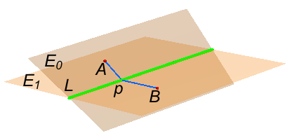
Figure 1. The metric space $E_{L}$

We define the metric on $E_{L}$ in terms of the minimizing geodesics between two points. If the two points lie in the same sheet then the geodesic between them is simply the usual line segment of $E$ which joins them, viewed as lying in their shared sheet. If the two points $A$ and $B$ lie in different sheets, the only way we can travel from $A$ to $B$ is by passing through $L$ to cross from one sheet to another. We are led to the problem of minimizing the distance from $A$ to $B$, in $E$, among all paths which touch $L$ in between. In other words, we must minimize $S_{AB}(p)=|A-p|+|p-B|$ over $p\in L$. As we have seen, there is a unique minimizer $p_{*}\in L$. Then the geodesic $AB$ consists of the union of the line segment $Ap_{*}$ in $A$’s sheet and the segment $p_{*}B$ in $B$’s sheet. The minimization problem is the same problem we encountered earlier. The geodesics in this case are in bijection with the point billiard trajectories having itinerary $(L)$.

This construction of $E_{L}$ is a special case of a general metric gluing procedure which is the subject of a theorem by Reshetnyak. In order to describe Reshetnyak’s theorem we must recall what it means for a metric space to be “CAT(0)” and “Hadamard”.

Let $(X,d)$ be a path-connected metric space. We define the length of a path in $X$ by taking infimums of “polygonal approximations” to the path (see [BBI, Def. 2.3.1.]). $X$ is called a length space if the distance $d(A,B)$ between points $A,B\in X$ is realized as the infimum of the lengths of paths between $A$ and $B$. If $X$ is also complete, then there is a shortest such path, denoted $AB$, and its length is $d(A,B)$. We call $AB$ a geodesic segment. (There may be more than one geodesic segment joining $A$ and $B$.) A triangle $\Delta ABC$ in $X$ is a subset consisting of three points $A,B,C\in X$ together with geodesic segments $AB,AC,BC$ joining them. A Euclidean comparison triangle $\Delta\bar{A}\bar{B}\bar{C}\subset\mathbb{R}^{2}$ for $\Delta ABC$ is a triangle in the Euclidean plane whose sides are congruent to those of $\Delta ABC$: $d(A,B)=\|\bar{A}-\bar{B}\|$, $d(A,C)=\|\bar{A}-\bar{C}\|$ and $d(A,C)=\|\bar{B}-\bar{C}\|$. If $x\in AB$ is a point on side $AB$, then there is a unique comparison point $\bar{x}\in\bar{A}\bar{B}$ defined by $\|\bar{A}-\bar{x}\|=d(A,x)$ , $\|\bar{x}-\bar{B}\|=d(x,B)$.

Definition 6.

[BBI, Defs. 4.1.9, 9.2.1.]) A CAT(0) space – also known as a space with non-positive curvature – is a complete length space $(X,d)$ such that every sufficiently small triangle $\Delta ABC$ in $X$ satisfies the following triangle comparison property. Let $\Delta\bar{A}\bar{B}\bar{C}$ be a Euclidean comparison triangle for $\Delta ABC$. If $x\in AB$ and $\bar{x}\in\bar{A}\bar{B}$ is the comparison point then $d(x,C)\leq\|\bar{x}-\bar{C}\|$.

Definition 7.

[BBI, Defs. 4.1.9, 9.2.1.] A Hadamard space is a simply-connected CAT(0) space.

The CAT(0) condition generalizes the Riemannian geometry condition that all sectional curvatures are non-positive to the case of (possibly) non-smooth metric length spaces. The fiducial example of a Hadamard space is a Euclidean space. Hyperbolic space and metric trees are other examples.

Theorem 4.

(Reshetnyak [BBI, 9.1.21.]) If $X_{1}$ and $X_{2}$ are Hadamard spaces containing isometric copies of the same convex set $K$, then the length space $X_{1}\cup_{k}X_{2}$ constructed by gluing $X_{2}$ to $X_{1}$ along $K$ is again a Hadamard space.

Reshetnyak’s theorem asserts that the output of gluing Hadamard spaces serves as another input! We can iterate. If $L_{1}L_{2}\ldots L_{k}$ is an itinerary we thus form the Hadamard “itinerary” space

$$E_{L_{1}L_{2}\ldots L_{k}}=E_{0}\cup_{L_{1}}E_{1}\cup_{L_{2}}\cup\ldots\cup_{L_{k}}E_{k}.$$

Point billiard trajectories having itinerary $L_{1}L_{2}\ldots L_{k}$ yield geodesics which connect the first sheet $E_{0}$ to the last sheet $E_{k}$.

Caveat. There may be minimizing geodesics in this Hadamard itinerary space which are not point billiard trajectories. These will be minimizers of $S_{AB}$ having either a multiple collision point $q_{i}=q_{i+1}$ or an edge lying within an $L_{i}$.

Proof of theorem 3. When $X$ is Hadamard there is a unique geodesic $AB$ joining any two points $A,B\in X$. See, for example, Theorem 9.2.2 of [BBI]. $\Box$

5. The Hessian

Proof of Proposition 2.

We continue with the same notation used in the proof of Proposition 1 as above (subsection 3.1), except now we add the shorthand:

(14) $$n_{i,j}=n(q_{i},q_{j})\quad;\quad r_{i,j}=|q_{i}-q_{j}|.$$

Write $d^{2}f$ for the Hessian of a function. Returning to the function $|x|$ on $E$, a routine computation shows that

$$d^{2}r=\frac{1}{r}|dx-\langle n,dx\rangle n|^{2};\qquad n=x/r.$$

An application of the chain rule now shows that

$$d^{2}r_{12}=\frac{1}{r_{12}}|(dq_{1}-dq_{2})-\langle n_{12},(dq_{1}-dq_{2})\rangle n_{12}\Big{|}^{2}$$

which simply means that

$$(d^{2}r_{12})_{(q_{1},q_{2})}(\xi_{1},\xi_{2})=\frac{1}{r_{12}}\big{|}(\xi_{1}-\xi_{2})-\langle n_{12},(\xi_{1}-\xi_{2})\rangle n_{12}\big{|}^{2}$$

as a quadratic form on $E\times E$.

It follows that

$$d^{2}S_{A,B}=\sum_{i=0}^{k}\frac{1}{r_{i,i+1}}\big{|}(dq_{i}-dq_{i+1})-\langle(dq_{i}-dq_{i+1}),n_{i,i+1}\rangle n_{i,i+1}\big{|}^{2},$$

provided we set $q_{0}=A$, $q_{k+1}=B$, $dq_{0}=0,dq_{k+1}=0$. In other words

(15) $$d^{2}S_{A,B} = \sum_{i=0}^{k}\frac{1}{r_{i,i+1}}\big{|}(\xi_{i}-\langle\xi_{i},n_{i,i+1}\rangle n_{i,i+1})-(\xi_{i+1}-\langle\xi_{i+1},n_{i,i+1}\rangle n_{i,i+1})\big{|}^{2}$$

is the Hessian $d^{2}S_{A,B}(\xi,\xi)$, a quadratic form in $\xi=(\xi_{0},\xi_{1},\ldots,\xi_{k},\xi_{k+1})$ where we set $\xi_{0}=\xi_{k+1}=0$, and where $\xi_{i}\in L_{i}$, $1\leq i\leq k$.

Expand out this Hessian, focussing on the block diagonal terms:

$$d^{2}S_{A,B}=\sum\frac{|\xi_{i}-\langle\xi_{i},n_{i,i+1}\rangle n_{i,i+1}|^{2}}{r_{i,i+1}}+\frac{|\xi_{i}-\langle\xi_{i},n_{i-1,i}\rangle n_{i-1,i}|^{2}}{r_{i-1,i}}+\text{ off-diagonal blocks}.$$

Since $Aq_{1}\ldots q_{k}B$ is a point billiard trajectory the projections of $n_{i-1,i}$ and $n_{i,i+1}$ onto $L_{i}$ are equal and so

$$|\xi_{i}-\langle\xi_{i},n_{i,i+1}\rangle n_{i,i+1}|^{2}=|\xi_{i}-\langle\xi_{i},n_{i-1,i}\rangle n_{i-1,i}|^{2}=|\xi_{i}|^{2}-\langle\xi_{i},a_{i}\rangle^{2}$$

where we have written:

$$\pi_{i}(n_{i-1,i})=\pi_{i}(n_{i,i+1}):=a_{i}\,.$$

We define this common quadratic form on $L_{i}$ to be:

$$\|\xi_{i}\|_{i}^{2}=|\xi_{i}-\langle\xi_{i},n_{i,i+1}\rangle n_{i,i+1}|^{2}=|\xi_{i}|^{2}-\langle\xi_{i},a_{i}\rangle^{2}$$

and we observe that it defines a new inner product on $L_{i}$. Indeed since $|a_{i}|<1$ (equivalently $n_{i,i+1}$, $n_{i-1,i}$ are unit vectors and are not in $L_{i}$), this quadratic form is indeed that of a positive definite inner product on $L_{i}$. Setting:

$$\beta_{i}=\frac{1}{r_{i-1,i}}+\frac{1}{r_{i,i+1}}$$

we see that

$$d^{2}S_{A,B}=\Sigma\beta_{i}\|\xi_{i}\|_{i}^{2}\ +\text{ off-diagonal}.$$

We proceed to understand the off-diagonal terms. After polarizing the quadratic form $d^{2}S_{A,B}$ to obtain the associated symmetric bilinear form, still denoted $d^{2}S_{A,B}$ we find that the off diagonal blocks are expressed in terms of the bilinear forms

$$Q_{ij}(\xi_{i},\zeta_{j})=\big{\langle}\xi_{i}-\langle\xi_{i},n_{i,j}\rangle n_{i,j}\ ,\ \zeta_{j}-\langle\zeta_{j},n_{i,j}\rangle n_{i,j}\big{\rangle},\quad\text{with}\quad|i-j|=1$$

with $\xi_{i}\in L_{i}$, $\zeta_{j}\in L_{j}$ and so $Q_{ij}$ is an “off-diagonal” bilinear form:

$$Q_{ij}:L_{i}\times L_{j}\to\mathbb{R}.$$

Then the off-diagonal terms of the polarized Hessian are:

$$\text{off-diagonal terms}=-\sum_{|i-j|=1}\frac{1}{r_{ij}}Q_{ij}(\xi_{i},\zeta_{j}).$$

Now, using our $\langle\cdot,\cdot\rangle_{i}$ inner products we have that

$$|Q_{ij}(\xi_{i},\zeta_{j})|\leq\|\xi_{i}\|_{i}\,\|\zeta_{j}\|_{j}$$

according to the usual Cauchy-Schwartz inequality on $E$. It follows that if we define the operators $S_{ij}:L_{j}\to L_{i}$ by

$$Q_{ij}(\xi_{i},\zeta_{j})=\langle\xi_{i},S_{ij}\zeta_{j}\rangle_{i}\,,$$

then the operator norms of the $S_{ij}$ are

(16) $$\|S_{ij}\|\leq 1$$

relative to the norms $\|\cdot\|_{i}$, $\|\cdot\|_{j}$.

Endow $\Lambda=L_{1}\times L_{2}\times\ldots L_{k}$ with the inner product $\langle\cdot,\cdot\rangle_{*}$ whose squared norm is $\Sigma\|\xi_{i}\|_{i}^{2}$. Then we can define a $\langle\cdot,\cdot\rangle_{*}$–symmetric matrix $M:\Lambda\to\Lambda$ in the usual way:

$$d^{2}S(\xi,\zeta)=\langle\xi,M\zeta\rangle_{*}$$

and we find that $M$ is block-tridiagonal with form:

(17) $$M=\left(\begin{array}[]{cccccc}\beta_{1}&-\frac{1}{r_{12}}S_{12}&0&0&\cdots&0\\ -\frac{1}{r_{21}}S_{21}&\beta_{2}&-\frac{1}{r_{23}}S_{23}&0&\cdots&0\\ 0&-\frac{1}{r_{23}}S_{32}&\beta_{3}&-\frac{1}{r_{34}}S_{34}&0&\cdots\\ \vdots&\vdots&\vdots&\vdots&\vdots\\ 0&0&\cdots&0&-\frac{1}{r_{k-1,k}}S_{k,k-1}&\beta_{k}\end{array}\right)\ .$$

In what follows, it is crucial to observe that the coefficients in all the rows but the first and last satisfy a simple linear condition:

$$\frac{1}{r_{i,i-1}}+\frac{1}{r_{i,i+1}}=\beta_{i}.$$

In order to establish that $M$ is invertible and hence $d^{2}S$ is nondegenerate we form

$$P=DM$$

where $D$ is the block-diagonal matrix whose $i$th block is $\frac{1}{\beta_{i}}$. Thus $D$ is the matrix for the invertible transformation $(D\xi)_{i}=\frac{1}{\beta_{i}}\xi_{i}$. Proposition 2 will be established once we establish the following lemma 1. $\Box$

Lemma 1.

$P$ is invertible.

Proof. We compute that

$$P=I-A$$

where $I$ is the identity and $A$ is tridiagonal block matrix with $0$’s on the diagonal and

(18) $$A=\left(\begin{array}[]{cccccc}0&b_{1}S_{12}&0&0&\cdots&0\\ a_{2}S_{21}&0&b_{2}S_{23}&0&\cdots&0\\ 0&a_{3}S_{32}&0&b_{3}S_{34}&0&\cdots\\ \vdots&\vdots&\vdots&\vdots&\vdots\\ 0&0&\cdots&0&a_{k}S_{k,k-1}&{0}\end{array}\right)$$

where $a_{i}=\frac{r_{i,i+1}}{r_{i,i-1}+r_{i,i+1}}$, $b_{i}=\frac{r_{i,i-1}}{r_{i,i-1}+r_{i,i+1}}$ so that

$$0<a_{i},b_{i}<1,\text{ and }a_{i}+b_{i}=1.$$

To prove that $P$ is invertible is equivalent to proving lemma 2 immediately below. $\Box$

Lemma 2.

$1$ is not an eigenvalue of $A$.

remark The argument underlying lemma 2 was inspired by playing with the situation in which all the $S_{i,j}=1$ so that $A$ becomes a tri-diagonal matrix with $0$’s on the diagonal, all other tridiagonal entries positive, and all of its row sums except the first and last being $1$, that is, a Perron-Frobenius matrix.

Proof of lemma 2. Introduce the new norm on $\oplus L_{i}$:

$$\|\xi\|^{*}:=\max_{j}\|\xi_{j}\|_{j}\,.$$

Suppose that $A\xi=\xi$. We must show that $\xi=0$. The eigenvalue equation reads:

$$\xi_{i}=a_{i}S_{i,i-1}\xi_{i-1}+b_{i}S_{i,i+1}\xi_{i+1},\quad 1<i<k$$

together with

$$\xi_{1}=b_{1}S_{1,2}\xi_{2}\quad\mbox{and}\quad\xi_{k}=a_{k}S_{k,k-1}\xi_{k-1}.$$

By way of contradiction, suppose that $\xi\neq 0$ so that $\|\xi\|^{*}>0$. Let $i$ be an index such that

$$\|\xi\|_{i}=\max_{j}\|\xi_{j}\|_{j}:=\|\xi\|^{*}\,.$$

Then $i$ cannot be $1$ or $k$, for if it were, taking norms of the eigenvalue equation for these indices and use eq (16), together with $|b_{1}|,|a_{k}|<1$ we would have $\|\xi\|^{*}<\|\xi\|^{*}$, a contradiction. So $1<i<k$. Taking norms we get

$$\|\xi_{i}\|_{i}\leq a_{i}\|S_{i,i-1}\xi_{i-1}\|_{i}+b_{i}\|S_{i,i+1}\xi_{i+1}\|_{i}\leq a_{i}\|\xi_{i-1}\|_{i-1}+b_{i}\|\xi_{i-1}\|_{i-1}\,.$$

Now $\|\xi_{i\pm 1}\|_{i\pm 1}\leq\|\xi\|_{i}$ and $a_{i}+b_{i}=1$. It follows that unless both $\|\xi_{i-1}\|_{i-1}$ and $\|\xi_{i+1}\|_{i+1}$ are equal to $\|\xi_{i}\|_{i}$ we will have again that $\|\xi\|^{*}<\|\xi\|^{*}$, a contradiction. Thus we have now have that

$$\|\xi\|^{*}=\|\xi_{i}\|_{i}=\|\xi_{i}\|_{i-1}=\|\xi_{i}\|_{i+1}.$$

Continuing in this manner we march up or down the indices until eventually $\|\xi_{1}\|_{1}=\|\xi_{k}\|_{k}=\|\xi\|^{*}$ and we return to our original contradiction.

Finally that the Hessian is positive definite and not simply nondegenerate follows from theorem 3, and hence the CAT(0) ideas of 4. $\Box$

6. Thickening

In this section we thicken each subspace $L\in{\mathcal{L}}$ and in so doing obtain an approximating deterministic dynamics to our point billiard system. We introduce the notion of trajectories being transverse. We prove that every transverse point billiard solution in ${\mathcal{B}}(L_{1}\ldots L_{k})$ is the limit of a family of thickened billiard trajectories as the thickening parameter tends to zero. This limit assertion yields another perspective on point billiards as well as a new proof of the main parts of theorems 1 and 2.

Definition 8.

Choose positive scale factors $\sigma_{L}>0$ for each $L\in{\mathcal{L}}$. For $r>0$ , $L\in{\mathcal{L}}$ set

$$L^{(r)}:=\{q\in E\mid d(q,L)\leq\sigma_{L}r\},$$

$$Z^{(r)}:=\{q\in E\mid d(q,L)=\sigma_{L}r\},\qquad\mbox{and}$$

$$\qquad{\mathcal{M}}^{(r)}:={\rm cl}\big{(}E-\textstyle\bigcup_{L\in{\mathcal{L}}}L^{(r)}\big{)}.$$

An “r-thickened billiard trajectory” is a solution $q^{(r)}$ to the deterministic billiard problem played on the table ${\mathcal{M}}^{(r)}$.

The walls of our table ${\mathcal{M}}^{(r)}$ are the unions of the cylindrical hypersurfaces $Z^{(r)}$ minus certain small ‘corner’ or intersection parts where two or more of the interiors $L^{(r)}$ of these cylinders intersect. Away from these small corners, the $r$-thickened billiard problem is a deterministic dynamics of standard billiard type.

Example 2 (Thickened $N$-body billiards = ideal gas).

The reason behind the scale factors in definition 8 arises here. The formula

(19) $$\sigma_{ab}r_{ab}={\rm dist}_{E}(q,\Delta_{ab});\qquad\sigma_{ab}=\sqrt{\frac{m_{a}+m_{b}}{m_{a}m_{b}}}.$$

relates the usual distance $r_{ab}=|q_{a}-q_{b}|$ between the $a$th and $b$th bodies and the $E$-distance between the corresponding configuration point $q=(q_{1},\ldots,q_{N})\in E=(\mathbb{R}^{d})^{N}$ and the collision subspace $\Delta_{ab}$ (See, for example, the proof of lemma 2 and eq (4.3.15a) in [Mont].) If we take $\sigma_{ab}$ for each $L=\Delta_{ab}$ in definition 8 then the domain ${\mathcal{M}}^{(r)}$ within which the thickened billiard moves is precisely the configuration space of $N$ hard balls with centers $q_{a}$ and radii $r/2$, that is, an ideal gas (but unconfined to a box).

Definition 9.

If $q$ is a point billiard solution then an $r$–family for $q$ is a family of r-thickened billiard trajectories $q^{(r)}:\mathbb{R}\to{\mathcal{M}}^{(r)}$, $r\leq r_{0}$, some $r_{0}>0$, such that $q^{(r)}\to q$ in the compact-open topology as $r\to 0$.

We would like to say that every point billiard trajectory admits an $r$-family. But that is not true. However the exceptional trajectories are quite easy to understand. Our reflection rule (eq 5) allows for point billiard trajectories which pass right through a collision subspace without changing direction: $n_{i-1,i}=n_{i,i+1}$. For deterministic billiards this cannot happen: collisions with walls change direction.

Definition 10.

   
An internal vertex of a polygonal path $q_{0}q_{1}\ldots q_{k}q_{k+1}$ is a vertex $q_{i}$ such that the edges $q_{i-1}q_{i}$ and $q_{i}q_{i+1}$ incident to it form a line segment $q_{i-1}q_{i+1}$ with $q_{i}$ in the interior. A polygonal path is transverse if it has no internal vertices.

Here is the main result of this section.

Proposition 3.

Any transverse point billiard trajectory $q$ admits an $r$–family $q^{(r)}$.

Basic remark. The itineraries of each path in the $r$–family agree with those of their limit $q$, for all $r$ small enough.

Caveat. The set of transverse billiard trajectories need not be dense within the set of all billiard trajectories realizing a given itinerary.

Example 3.

If $L\in{\mathcal{L}}$ has codimension one then ‘half’ of the transverse billiard trajectories colliding with $L$ are scattered back into the same half space of $E\setminus L$ while the other half pass straight thru $L$ without their direction of travel being altered. So the transverse $L$-colliding trajectories are not transverse.

Example 4.

If three consecutive different scattering subspaces $L_{i-1}$, $L_{i}$ and $L_{i+1}$ are coplanar lines then any trajectory which has $L_{i-1}L_{i}L_{i+1}$ as part of its itinerary will have $n_{i-1,i}=n_{i,i+1}$ and hence is not transverse.

Our proof of proposition 3 relies on a minimizing property of thickened billiard trajectories quite similar to that used for our earlier point billiards arguments but with one crucial difference. The difference is the existence of “ghost billiards”. (See lemma 4.)

Thicken our old parameter space to

$$\Lambda^{(r)}=L_{1}^{(r)}\times\cdots\times L_{i}^{(r)}\times\cdots\times L_{k}^{(r)}.$$

and consider the polygonal path length function with $\Lambda^{(r)}$ as the input vertices to form the thickened analogue of $S_{AB}$.

Lemma 3.

For fixed $A,B\in int({\mathcal{M}}^{(r)})$ the minimum of $S_{A,B}$ over $\lambda^{(r)}\in\Lambda^{(r)}$ exists and is unique. Moreover, any local minimizer or critical point for $S_{AB}$ is this global minimizer. If that global minimizer is transverse then it is a solution to the deterministic billiard problem in $int({\mathcal{M}}^{(r)})$. Conversely, any solution to the deterministic billiard problem is a minimum of $S_{AB}$ where $A,B$ are taken on the incoming and outgoing rays of the solution.

Lemma 4 (Ghost Billiards).

There exist non-transverse minimizers. For these, the interior vertex $q_{i}^{(r)}$ is part of a line segment $q_{i-1}q_{i+1}^{(r)}$ which is either tangent to $Z_{i}^{r}$ at $q_{i}^{(r)}$ or (the more important case) which passes through the interior of $L_{i}^{(r)}$ so that $q_{i}^{(r)}$ may be taken to lie in that interior, in which case we say that the minimizer is a “ghost billiard trajectory” in honor of what such a trajectory looks like in the thickened $N$-body billiards case.

Proof of lemma 3. With the exception of the assertion regarding transverse minimizers, the proof of lemma 3 is almost identical to the proof of the minimization property which we gave above in propositions 1 and 2 for point billiard trajectories. A proof can also be found in [BFK1]. The unique global minimization property of $S_{AB}$ is achieved in a manner identical to our proof of theorem 3. We form Hadamard spaces by gluing sheets $E_{i}=E$ together, now along the convex bodies $L_{i}^{(r)}$. To understand the assertion regarding transverse minimizers within the lemma we must understand a bit about the ghost billiards of lemma 4.

Sketch, Proof of lemma 4. Take the case of a single $L$, that is, of an itinerary of length 1. Set $K=L^{(r)}$, a convex body with non-empty interior in $E$. Suppose that the line segment $AB$ passes through the interior of $K$. Put $A\in E_{0}$ and $B\in E_{1}$ in the gluing construction $E_{0}\cup_{K}E_{1}$ of Reshetnyak’s theorem. The geodesic from $A$ to $B$ is now the straight line segment $AB$ passing through the convex body without being deflected and still passing from one sheet to the other. This is our ghost geodesic! Take $q_{1}\in AB\cap K$ when minimizing the thickened $S_{AB}$ to arrive at the non-transverse minimizer $Aq_{1}B$. If, on the other hand, a minimizer is transverse it cannot be a ghost billiard (nor can it be a billiard with a tangency to $K$). Such a transverse minimizer must correspond to an “honest billiard” - a solution to the deterministic billiard system.

Proof of Proposition 3. Let $q$ be a transverse point billiard trajectory with vertices $q_{i}\in L_{i}$ listed in order. Choose points $q_{0}=A$ and $q_{k+1}=B$ on the ingoing and outgoing rays. By a slight abuse of notation, we will also write $q$ for that finite part of $q$ joining $A$ to $B$. Let ${\mathcal{P}}_{0}$ denote the space of polygonal paths $q^{\prime}$ starting at $A$, ending at $B$ and having $k$ vertices $q^{\prime}_{i}\in L_{i}$ in between, listed in order. Then $q\in{\mathcal{P}}_{0}$. According to the set-up from the beginning of section 3, ${\mathcal{P}}_{0}$ is naturally isomorphic to the parameter space $\Lambda$ and $S_{AB}$ is the restriction of the length functional $\ell$ to ${\mathcal{P}}_{0}$. Proposition 1 and theorem 3 assert that $q$ is the global minimum of $S_{AB}$. Write $T=S_{AB}(q)$ for this minimum value. (Thus, since $q$ is parameterized by arclength if $q(0)=A$ we have that $q(T)=B$.)

Claim 1. There is a small positive constant $\delta_{0}$ and a positive constant $K$ with the following significance. If $\delta<\delta_{0}$ and if $q^{\prime}\in{\mathcal{P}}_{0}$ has the property that one of its $k$ corners $q^{\prime}_{i}$ satisfies $|q^{\prime}_{i}-q_{i}|\geq\delta$ then $\ell(q^{\prime})\geq T+K\delta^{2}$.

Write ${\mathcal{P}}(r)$ for the space of polygonal paths starting at $A$, ending at $B$ and having $k$ vertices $q^{\prime\prime}_{i}\in Z_{i}(r)=\partial L_{i}^{(r)}$. For $q^{\prime\prime}\in{\mathcal{P}}(r)$ we write $\pi(q^{\prime\prime})\in{\mathcal{P}}_{0}$ for the polygonal path whose $k$ vertices are $q^{\prime}_{i}=\pi_{i}(q^{\prime\prime}_{i})\in L_{i}$ where $\pi_{i}:E\to L_{i}$ is the orthogonal projection.

Claim 2. Suppose that $\delta,\delta_{0}$ and $K$ are as in Claim 1. Take $r_{0}>0$ such that $2\Sigma\sigma_{i}r_{0}<K\delta^{2}/2$ where $\sigma_{i}=\sigma_{L_{i}}$ are the scale factors attached to $L_{i}$ as per definition 8. If $r<r_{0}$ and $q^{\prime\prime}\in{\mathcal{P}}(r)$ is such that $\pi(q^{\prime\prime})\in{\mathcal{P}}_{0}$ satisfies the hypothesis of claim 1 (i.e. $|q^{\prime}_{i}-q_{i}|\geq\delta$ for some $i$) then $\ell(q^{\prime\prime})>T+K\delta^{2}/2$.

Claim 3. [Curve Shortening] For any $q\in{\mathcal{P}}_{0}$ and any $r$ sufficiently small there is a $q^{\prime\prime}\in{\mathcal{P}}(r)$ with $\ell(q^{\prime\prime})<\ell(q)$.

We now show how the three claims yield the lemma. Afterwards we prove the claims. By lemma 3 for all $r$ there exists a unique length minimizer $q_{*}=q_{*}^{(r)}\in{\mathcal{P}}(r)$. Apply the curve shortening process of Claim 3 to $q$ in order to get a $q^{\prime\prime}\in{\mathcal{P}}(r)$ with $\ell(q^{\prime\prime})<T=\ell(q)$. Thus $\ell(q_{*})\leq\ell(q^{\prime\prime})<\ell(q)=T<T+(K/2)\delta^{2}$. Take $\delta,\delta_{0},r_{0},r$ as per claim 2 to conclude that each vertex $q^{\prime}_{i}$ of the projected polygonal curve $q^{\prime}=\pi(q_{*})\in{\mathcal{P}}_{0}$ satisfies $|q^{\prime}_{i}-q_{i}|<\delta$. But $|q_{*i}-q_{i}|=\sqrt{|q_{*i}-q^{\prime}_{i}|^{2}+|q^{\prime}_{i}-q_{i}|^{2}}=\sqrt{\sigma_{i}^{2}r^{2}+|q^{\prime}_{i}-q_{i}|^{2}}<\sqrt{2}\delta$ where in the first equality we used the fact that $q^{\prime}_{i}=\pi_{i}(q_{*i})$ is the orthogonal projection onto $L_{i}$. Letting $\delta\to 0$ we get that $q_{*i}\to q_{i}$. Since $q$ is transverse, eventually, for $r$ small enough, $q_{*}$ is also transverse, and hence a thickened billiard solution. This proves that the $q_{*}$ form an $r$-family for $q$.

It remains to prove the three claims.

Proof of Claim 1. (i) Since the Hessian of $S_{AB}$ is positive definite at $q$ (proposition 2) we have that there exists a $\delta_{1}>0$ such that whenever $q^{\prime}\in{\mathcal{P}}_{0}$ satisfies $|q^{\prime}_{i}-q_{i}|<\delta_{1}$ for all $i$ then $S_{AB}(q^{\prime})-S_{AB}(q)\geq\Sigma_{i}K|q^{\prime}_{i}-q_{i}|^{2}$. Our $\delta_{0}$ will eventually be less than or equal to $\delta_{1}$.

(ii) Now if $q^{\prime}\in{\mathcal{P}}_{0}$ has any vertex $q^{\prime}_{i}$ such that $|q^{\prime}_{i}-q_{0}|\geq T+K\delta_{1}^{2}$ then $\ell(q^{\prime})>T+K\delta_{1}^{2}$.

(iii) Now restrict the length functional to the compact set of paths $q^{\prime}\in{\mathcal{P}}_{0}$ all of whose vertices $q^{\prime}_{i}$ satisfy $|q^{\prime}_{i}-q_{i}|\leq T+K\delta_{1}^{2}$ and at least one of which satisfies $|q^{\prime}_{i}-q_{i}|\geq\delta_{1}$. This set of polygonal paths is naturally homeomorphic to a compact subset of $\Lambda$, and as such the length functional $S_{AB}$ achieves its minimum value $T_{M}=\ell(q_{M})$ on the set. $T_{M}>\ell(q)=T$ because $q$ is the unique global minimizer of $S_{AB}$ and $q$ is not in our compact set. Write $T_{M}=T+\epsilon_{M}$ to get that $\ell(q^{\prime})>T+\epsilon_{M}$ for all the paths in this compact set. (We have $\epsilon_{M}\leq\delta_{1}$.)

Combining (iii) and (ii) we see that if any path $q^{\prime}\in{\mathcal{P}}_{0}$ has one vertex $q^{\prime}_{i}$ with $|q^{\prime}_{i}-q_{i}|\geq\delta_{1}$ then $\ell(q^{\prime})\geq T+\min\{\epsilon_{M},K\delta_{1}^{2}\}$. Choose $\delta_{0}$ so that $\min\{\epsilon_{M},K\delta_{1}^{2}\}=K\delta_{0}^{2}$. This $\delta_{0}$ will do the needed trick. For let $\delta\leq\delta_{0}$ and suppose that $q^{\prime}$ has one vertex $q^{\prime}_{i}$ with $|q^{\prime}_{i}-q_{i}|\geq\delta$. Let $i$ be an index such that $|q^{\prime}_{i}-q_{i}|$ is maximized and let this maximum value be $m$. Thus $m\geq\delta$. If $m\geq\delta_{1}$, then from the previous paragraph $\ell(q^{\prime})\geq T+\min\{\epsilon_{M},K\delta^{2}\}=T+K\delta^{2}$. Otherwise, $m<\delta_{1}$ and the Hessian bound holds on $q^{\prime}$, yielding $\ell(q^{\prime})\geq T+K\Sigma_{i}|q^{\prime}_{i}-q_{i}|^{2}\geq T+Km^{2}\geq T+K\delta^{2}$. $\Box$.

Proof of Claim 2.

Suppose that $q^{\prime\prime}$ is as in the statement of this claim so that its projection $q^{\prime}$ satisfies the conditions of Claim 1 and thus $\ell(q^{\prime})\geq T+K\delta^{2}$. The difference between the vertices of $q^{\prime\prime}$ and $q^{\prime}$ satisfies $|q^{\prime\prime}_{i}-q^{\prime}_{i}|=\sigma_{i}r^{2}$ since the projection $\pi_{i}$ is orthogonal and $q^{\prime\prime}_{i}\in Z_{i}(r)$. By the triangle inequality $|q^{\prime}_{i}-q^{\prime}_{i+1}|-\sigma_{i}r-\sigma_{i+1}r\leq|q^{\prime\prime}_{i}-q^{\prime\prime}_{i+1}|$ so that

$$T+K\delta^{2}\leq\ell(q^{\prime})-2\Sigma\sigma_{i}r\leq\ell(q^{\prime\prime}).$$

By assumption $2\Sigma\sigma_{i}r\leq(K/2)\delta^{2}$, yielding the desired result,

$$T+(K/2)\delta^{2}\leq\ell(q^{\prime\prime})$$

Proof of Claim 3. For each vertex $q_{i}$ consider the triangle $\Delta_{i}$ whose vertices are $q_{i-1},q_{i},q_{i+1}$. By the transversality condition $\Delta_{i}$ is a nondegenerate triangle and so lies in a unique affine planes $P_{i}\subset E$. The solid cylinder $L_{i}(r)$ intersects $P_{i}$ in a convex domain $K_{i}(r)$ (the interior of an ellipse) containing the vertex $q_{i}$, and for $r$ sufficiently small the other two vertices of our triangle are not in $K_{i}(r)$. See figure 2. $K_{i}(r)\cap\Delta_{i}\subset P_{i}$ is a convex planar domain whose boundary consists of three arcs, two being line segments forming part of the edges of $\Delta_{i}$ and the third curved arc $C_{i}$ (a subarc of the ellipse) lying in the interior of $\Delta_{i}$. Choose any point $q^{\prime\prime}_{i}\in C_{i}$ on this third arc. Then $q^{\prime\prime}_{i}\in Z_{i}(r)$. But $q^{\prime\prime}_{i}$ is in the interior of our triangle, and so by a general property of interior points of triangles we have that $|q_{i-1}-q^{\prime\prime}_{i}|+|q^{\prime\prime}_{i}-q_{i+1}|<|q_{i-1}-q_{i}|+|q_{i}-q_{i+1}|$. See figure 2 again.

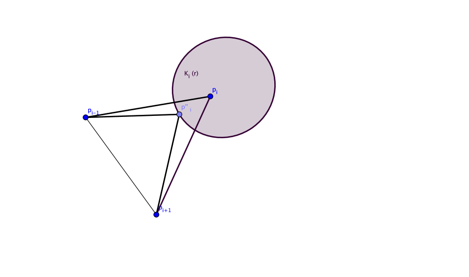
Figure 2. The curve shortening process of Claim 3

It follows that the replacement of vertex $q_{i}$ by $q^{\prime\prime}_{i}$ leaving all other vertices of $q$ unchanged shortens the polygonal path. Indeed, only the edge lengths of the two edges incident to the changed vertex change and the sum of these two decrease. Write this replacement process as $q\mapsto\sigma_{i}(q)$. Apply this polygonal curve shortening process consecutively, vertex-by-vertex, $q\mapsto\sigma_{1}(q)\mapsto\sigma_{2}(\sigma_{1}(q))\mapsto\ldots\mapsto\sigma_{k}(\ldots(\sigma_{1}(q))\ldots))=q^{\prime\prime}$. Each replacement shortens the path. The $k$th application yields a path $q^{\prime\prime}\in{\mathcal{P}}(r)$ all of whose corners $q^{\prime\prime}_{i}$ lie on their respective boundary sets $Z_{i}(r)$ and which is shorter than the original path $q$. $\Box$ (for the proof of Proposition 3).

6.1. Relation to proofs of theorems 1, 2

The $r$-thickened dynamics is deterministic and symplectic. The graph of its time $T$ flow is, morally speaking, a Lagrangian graph. This graph is partitioned up into pieces according to the itineraries of the trajectories. In some sense, which we are purposely vague on, our Lagrangian relations of theorems 1 and 2, are the limits $r\to 0$ and $T\to\infty$ of the pieces of this graph. Among the problems faced in turning this idea into a complete proof is the fact that the flow is not continuous due to the instantaneous velocity changes suffered at collisions.

7. Conservation Laws, Symmetries, and Scaling.

Solutions to the $N$-body problem enjoy conservation of linear and angular momentum. We expect that our $N$-body billiard trajectories to obey these same conservation laws. They do. We show derive the laws from the group invariance of the collision subspaces. We end this section with a remark on a scaling symmetry for billiard trajectories and what it implis for the closures of our Lagrangian relations in theorem 1.

7.1. Momentum maps for free motion and its restrictions.

The usual linear and angular momentum are the components of the momentum map for the group of rigid motions of the underlying Euclidean space. We take, to start with, the full group of rigid motions of our $E$, and later restrict to subgroups mapping the collision spaces to themselves.

The group ${\rm Iso}(E)$ of rigid motions of $E$ splits into translations and rotations. Write ${\rm Lie}({\rm Iso}(E))^{*}$ for the dual of the Lie algebra of this Lie group. Using the inner product on $E$ we have canonical identifications: $T^{*}E=E\times E$ and ${\rm Lie}({\rm Iso}(E))^{*}={\rm Lie}({\rm Iso}(E))=E\oplus\Lambda^{2}E$. The full momentum map is then the map $\Phi=(P,J):E\times E\to E\oplus\Lambda^{2}E$ whose first (translational) factor $P(x,v)=v$ we call the “full” linear momentum and whose second (rotational) factor $J_{\rm rot}(x,v)=x\wedge v$ we call the ‘full’ angular momentum and is that for the full rotation group.

Free (=straight line) motion $(x,v)\mapsto(x+tv,v)$ is a Hamiltonian flow on $E\times E$ which has the full momenta as conserved quantities.

Now restrict attention to the Lie subgroup of those $g\in{\rm Iso}(E)$ such that $g(L)=L$ for each $L\in{\mathcal{L}}$. Being a subgroup of ${\rm Iso}_{+}(E)$, this subgroup also acts symplectically on the phase space $E\times E$ and has its own momentum map which is well-known to be the composition of the previous full momentum map $\Phi$ with the orthogonal projection onto our subgroup’s Lie algebra. In this way we get linear and angular momenta associated to our collision-preserving subgroup. :

$$P_{\rm tr}(x,v)=\pi_{\rm tr}(v)\in L_{\rm tr}$$

and

$$J(x,v)=\pi(x\wedge v)\in{\rm Lie}(H)$$

where $\pi_{\rm tr}:E\to L_{\rm tr}$ projects onto the translational part of our subgroup and $\pi:\Lambda^{2}E\to{\rm Lie}(H)$ projects onto its rotational part. In the next two subsections we compute these projections and derive their conservation consequences.

7.2. Linear Momentum and Translation invariance

The translational part of our collision-preserving subgroup is:

(20) $$L_{\rm tr}=\bigcap_{L\in{\mathcal{L}}}L.$$

In other words, $L_{\rm tr}$ is precisely the subgroup of translations of $E$ which maps each $L$ onto itself. Write $\pi_{\rm tr}:E\to L_{\rm tr}$ for the orthogonal projection onto this subspace, as above, we have:

Proposition 4.

The ‘total linear momentum” $\pi_{\rm tr}(v)$ is constant along each billiard trajectory.

Proof. At each collision we have $\pi_{L}(v_{-})=\pi_{L}(v_{+})$. But $L_{\rm tr}\subset L$ for all $L\in{\mathcal{L}}$. So $\pi_{\rm tr}(v_{-})=\pi_{\rm tr}(v_{+})$ at each collision: the total momentum remains unchanged at each collision and thus $\pi_{\rm tr}(v)$ is constant along any given billiard trajectory. $\Box$

$N$-body billiard momentum conservation In $N$-body billiards the intersection of all of the $\Delta_{ij}$ consists of the $d$-dimensional subspace consisting of all vectors of the form $(z,z,\ldots,z)$, $z\in\mathbb{R}^{d}$. It is the subspace of $E=(\mathbb{R}^{d})^{N}$ generated by the translation group of $\mathbb{R}^{d}$. The projection of a velocity $v\in(\mathbb{R}^{d})^{N}$ onto this subspace, relative to the mass metric, is $(v_{1},\ldots,v_{N})\mapsto\Sigma m_{a}v_{a}$ which co-incides with total linear momentum.

7.3. Angular Momentum and Rotational Invariance

Now we consider the rotational part of our collision-preserving subgroup. Denote this subgroup as $H\subset{\rm O}(E)$ so that $H$ consists of all rotations which map the collision subspaces to themselves. We write $\pi_{H}:\Lambda^{2}E\to{\rm Lie}(H)$ for the orthogonal projection, identifying ${\rm Lie}(H)$ with a linear subspace of $\Lambda^{2}(E)$. Use the naturally induced invariant inner product on $\Lambda^{2}(E)$. On bivectors $v\wedge w$ the squared length for this inner product is

(21) $$\langle v\wedge w,v\wedge w\rangle=\det\left(\begin{array}[]{cc}\langle v,v\rangle&\langle w,v\rangle\\ \langle v,w\rangle&\langle w,w\rangle\end{array}\right)$$

Proposition 5.

The ‘total angular momentum” $\pi_{H}(x,v)$ is constant along each billiard trajectory.

Proof. Let $\xi\in{\rm Lie}(H)$. Thus $e^{t\xi}\in H$ is a one-parameter family of rotations leaving each $L$ invariant. The $\xi$-component of the full angular momentum is

$$J^{\xi}(x,v)=\langle x\wedge v,\xi\rangle$$

where $\langle\cdot,\cdot\rangle$ is the inner product on ${\rm so}(E)\cong\Lambda^{2}E$ just described. Since $x\wedge v$ is constant along straight line motions, $J^{\xi}(x,v)$ remains constant along the straight line segment parts of a billiard trajectory. We must show that it remains unchanged at collisions. The jump in $J^{\xi}$ at a collision with an $L$ at $q\in L$ is:

$$J^{\xi}(q,v_{+})-J^{\xi}(q,v_{-})=\langle q\wedge(v_{+}-v_{-}),\xi\rangle$$

Now from $\pi_{L}(v_{+})=\pi_{L}(v_{-})$ we have that $v_{+}-v_{-}\in L^{\perp}$. Thus $q\wedge(v_{+}-v_{-})\in L\wedge L^{\perp}\subset\Lambda^{2}E$. Our proposition now follows from the computational lemma:

Lemma 5.

If $\xi\in{\rm Lie}(H)$, $q\in L$ and $v\in L^{\perp}$ then $\langle q\wedge v,\xi\rangle=0$.

Proof of lemma. Using bilinearity of the inner product and formula (21) one verifies that for any $\xi\in\Lambda^{2}E$ we have

$$\langle q\wedge v,\xi\rangle=\langle\xi(v),q\rangle$$

where on the right-hand side we view are viewing $\xi$ as a skew symmetric map $\xi:E\to E$ using the canonical identification $\Lambda^{2}(E)\cong{\rm so}(E)$. (Under this identification the bivector $q\wedge v$ becomes the linear transformation $e\mapsto(q\wedge v)(e)=\langle v,e\rangle q-\langle q,e\rangle v$ of $E$.) It follows that we also have

$$\langle q\wedge v,\xi\rangle=-\langle\xi(q),v\rangle$$

Now if $\xi\in{\rm Lie}(H)$ then $e^{t\xi}\in H$ is a one-parameter family of rotations leaving each $L$ invariant. Differentiating, we see that if $q\in L$ then $\xi(q)\in L$. But in the lemma $v\in L^{\perp}$ so that $-\langle\xi(q),v\rangle=0$. $\Box$

$N$ body billiards. The group $H={\rm O}(d)$ acts diagonally on the $N$-body configuration space $(\mathbb{R}^{d})^{N}$ leaving each $\Delta_{ij}$ invariant. The mass-metric projection of $q\wedge v\in{\rm so}((\mathbb{R}^{d})^{N})={\rm so}(E)$ to ${\rm Lie}(H)=\Lambda^{2}\mathbb{R}^{d}$ is $\pi_{H}(q\wedge v)=\Sigma_{a=1}^{N}m_{a}q_{a}\wedge v_{a}\in\Lambda^{2}\mathbb{R}^{d}$, the usual formula for the total angular momentum. We have that total angular momentum is conserved for $N$-body billiards.

7.4. Scaling and the Scattering map as a Legendrian Map.

If $q(t)$ is a billiard trajectory with itinerary $L_{1}L_{2}\ldots L_{k}$ then so is $\lambda q(\frac{t}{\lambda}):=q_{\lambda}(t)$, $\lambda>0$. Letting $\lambda\to 0$ brings all the collision points $q_{i}$ of $q_{\lambda}$ to the origin. In this way we see that the closure of the Lagrangian relation $\mathcal{R}$ for ${\mathcal{B}}(L_{1}L_{2}\ldots L_{k})$ (see theorem 1) contains points lying in the Lagrangian relation for total collision described in example 1 - namely the product of the two zero sections of $T^{*}S(E)={\rm\it LINES}(E)$.

Scaling acts on pairs $(q,v)\in E\times E_{v}$ by $\lambda(q,v)=(\lambda q,v)$. Directions are left unchanged while ‘impact parameters’ $q$ are scaled. Let $\tilde{\mathcal{R}}=\tilde{\mathcal{R}}(L_{1}\ldots L_{k})$ be the “unreduced” Lagrangian relation of theorem 2. The scale invariance of ${\mathcal{B}}(L_{1}L_{2}\ldots L_{k})$ implies that $\tilde{\mathcal{R}}$ is scale-invariant: $(q_{A},v_{A}),(q_{B},v_{B})\in\tilde{\mathcal{R}}\iff((\lambda q_{A},v_{A}),(\lambda q_{B},v_{B}))\in\tilde{\mathcal{R}}$. In other words, the Lagrangian relation is a scale-invariant submanifold of $(E\times E_{v})\times(E\times E_{v})$.

Scaling commutes with reduction, and so induces a scaling action on $T^{*}S(E_{v})\times T^{*}S(E_{v})$ which leaves the Lagrangian relation ${\mathcal{R}}$ of theorem 1 invariant. In terms of the coordinates on $LINES(E)\cong T^{*}S(E_{v})$ discussed in subsection 1.2.6, scaling acts again by $(v,Q)\mapsto(v,\lambda Q)$. Thus we expect to be able to form the quotient by this action to arrive at a submanifold ${\mathcal{R}}/\mathbb{R}^{+}\subset(T^{*}S(E_{v})\times T^{*}S(E_{v}))/\mathbb{R}^{+}$. The latter is a nice manifold provided we delete its zero section before forming the scaling quotient. Indeed, for any manifold $X$, let $Z_{X}\subset T^{*}X$ denote the zero section of its cotangent bundle. Then $(T^{*}X\setminus Z_{X})/\mathbb{R}^{+}=\mathbb{P}(T^{*}X)$ is a canonical contact manifold which fibers over $X$ with fibers $\mathbb{R}\mathbb{P}^{n-1}$’s, $n=dim(X)$. (See [Arnold, Appendix 4].) We apply this observation to $X=S(E_{v})\times(S(E_{v})$, using $T^{*}(S(E_{v})\times T^{*}S(E_{v})=T^{*}(S(E_{v})\times(S(E_{v}))$ to arrive at:

Theorem 5.

If the itinerary has length greater than 1 then the quotient ${\mathcal{R}}/\mathbb{R}^{+}$ of the Lagrangian relation ${\mathcal{R}}$ of theorem 1 by the scaling group $\mathbb{R}^{+}$ is a submanifold of $\mathbb{P}T^{*}(S(E_{v})\times(S(E_{v}))$ of dimension $2dim(E)-3$ which is Legendrian relative to the (nonstandard) contact form

$$\Theta={\vec{Q}_{-}}\cdot d{\vec{v}_{-}}-{\vec{Q}+}\cdot d{\vec{v}_{+}}.$$

The projections to the incoming and outgoing velocity spheres are scale invariant maps and combine to yield the Legendrian fibration

$$\pi_{-}\times\pi_{+}:\mathbb{P}T^{*}(S(E_{v})\times(S(E_{v}))\to S(E_{v})\times S(E_{v})$$

under which the image of ${\mathcal{R}}/\mathbb{R}^{+}$ is a (possibly singular) hypersurface provided it is transverse to the fiber at some point

Proof. We first check that ${\mathcal{R}}$ does not intersect the zero section. If $Q=0$ then $0=q_{1}+tv_{-}$ which is only possible if either $q_{1}=0$ or $v_{-}\in L_{1}$ with $v_{-}=-q_{1}/t$. The latter is impossible since this would imply that the whole incoming line $\ell_{-}\subset L_{1}$. If the itinerary has length 2, the former is also possible, since if $q_{1}=0$, then $q_{1}\in L_{2}$ as well, which is excluded by our definition of belonging to ${\mathcal{B}}$. Thus the quotient ${\mathcal{R}}/\mathbb{R}^{+}$ is a well-defined submanifold of $\mathbb{P}T^{*}(S(E_{v})\times(S(E_{v}))$.

Next we check the Legendrian condition and at the same time work out the contact form. Write $D={\vec{Q}_{-}}{{\partial}\over{\partial\vec{Q}_{-}}}+{\vec{Q}_{-}}{{\partial}\over{\partial\vec{Q}_{-}}}$ for the Euler vector field, this being the vector field whose flow is dilation (with $\lambda=e^{t}$ if $t$ is the flow parameter). Let $\Omega=\omega_{-}-\omega_{+}$ be the symplectic form with respect to which ${\mathcal{R}}$ is Lagrangian. A standard construction from contact and symplectic geometry suggests forming the one-form $\Theta=i_{D}\Omega$ which a direct computation shows that $\Theta$ is the one-form stated in the theorem. Since ${\mathcal{R}}$ is scale invariant, $D$ is tangent to ${\mathcal{R}}$ and consequently $\Theta(v)=\Omega(D,v)=0$ for any other vector $v$ tangent to ${\mathcal{R}}$. This proves that ${\mathcal{R}}/\mathbb{R}^{+}$ is Legendrian relative to $\Theta$.

Finally, if ${\mathcal{R}}/\mathbb{R}^{+}$ is transverse to the fibers of the fibration, then $\pi_{-}\times\pi_{+}$ maps it locally diffeomorphically onto a hypersurface. The projection and ${\mathcal{R}}/\mathbb{R}^{+}$ are both algebraic so if the Legendrian submanifold is transverse at one point it is transverse at almost every point and the image of each component is a singular hypersurface. $\Box$

Remark.

If ${\mathcal{R}}/\mathbb{R}^{+}$ is nowhere transverse to the fiber then it is mapped to a subvariety of codimension greater than 1 within the product of the spheres.

Remark.

We can summarize the discussion of this subsection as saying that the map $q\mapsto(v_{-},v_{+})$ which sends a billiard trajectory to its incoming and outgoing velocities is a “Legendrian map”. Arnol’d [Arnold, Appendix 16, p. 487] calls the restriction of a Legendrian fibration to a Legendrian submanifold a “Legendrian map” and its image a “front” as in “wave-front. So the “scattering map” $\pi_{-}\times\pi_{+}$ restricted to ${\mathcal{R}}/\mathbb{R}^{+}$ is a Legendrian map and its image, the ‘scattering front’ will be an interesting singular hypersurface within the product of the incoming and outgoing velocity spheres. See subsection 8.2 below.

8. Examples

8.1. Origami unfoldings

Suppose that ${\mathcal{L}}$ consists of lines, so that $d=\dim(E)-1$. Let $q\in{\mathcal{B}}(L_{1}L_{2}\ldots L_{k})$ be a trajectory. Then each $q_{i}\in L_{i}$ is nonzero, for otherwise $q_{i}\in L_{i+1}$ which is forbidden. Assume $k>1$. Edge $q_{i}q_{i+1}$ of our $k+1$-gon $q$ joins the rays $\overrightarrow{0q_{i}}$ and $\overrightarrow{0q_{i+1}}$ and hence lies in the plane $P_{i}$ spanned by $0,q_{i},q_{i+1}$. Within this plane the edge lies within the sector $S_{i}$ bounded by these two rays. (By a “sector” we mean a planar convex region bounded by two rays.) Let $\theta_{i}={\rm angle}(q_{i}0q_{i+1})$ denote the opening angle of this sector. Thus the interior part $q_{1}q_{2}...q_{k}$ of our billiard trajectory lies on a polygonal cone within $E$ whose faces are the sectors $S_{1}\ldots S_{k-1}$ glued together along the rays $0q_{i}\subset L_{i}$. We can “unfold” this cone onto a fixed plane, thus forming a big sector which is made of congruent copies of our sectors $S_{1},S_{2},\ldots,S_{k-1}$ joined along their shared rays; see figure 3.

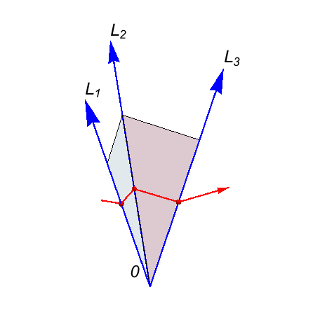
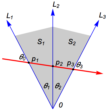
Figure 3. Left: Origami in $E$. Right: Origami unfolded

The opening angle of this big developed sector is

$$\beta=\theta_{1}+\theta_{2}+\ldots\theta_{k-1}.$$

Our billiard trajectory unfolds onto this developing plane as well. The billiard condition (1) is precisely that this unfolded trajectory is a straight line segment on this developing plane. To reiterate,
The billiard segment $q_{1}\ldots q_{k}$ becomes a straight line segment drawn on our big sector which is the flattened polyhedral cone!

Corollary 1.

If $\beta\geq\pi$ the alleged billiard trajectory does not exist.

Proof. For if a straight line enters in to one part of a sector through one ray boundary and leaves through the other ray boundary then the opening angle of the sector cannot be greater than $\pi$. Said differently, the developed sector will not be convex if $\beta>\pi$. $\Box$
Set $\beta_{i}={\rm angle}(L_{i},L_{i+1})$ so that $\beta_{i}$ is the minimum of $\theta_{i}$ and $\pi-\theta_{i}$. Thus $\beta\geq\Sigma\beta_{i}$.

Corollary 2.

Set $\theta_{\min}=\min({\rm angle}(L,M))$, the minimum taken over all $L,M\in{\mathcal{L}}$, $L\neq M$. There are no itineraries of length greater than $1+\lfloor\pi/\theta_{\min}\rfloor$.

Proof. Indeed since $\beta_{i}\geq\theta_{\min}$ we have that $\beta\geq(k-1)\theta_{\min}$ so that $\pi\geq(k-1)\theta_{\min}$ and thus the number of intersection $k$ satisfies $(\pi/\theta_{\min})\geq k-1$ . $\Box$
Projecting the incoming and outgoing velocities onto our developing plane we get information on their angles from the unfolded figure.

Corollary 3.

Consider the angle $\theta_{0}$ between the incoming ray (direction $v_{A}$) and the line $L_{1}$, the angle oriented so as to be the angle between $q_{1}$ and $-v_{A}$. Similarly consider the angle $\theta_{k}$ between the final collision line $L_{k}$ and the outgoing ray (direction $v_{B}$), that angle oriented so as to be between the vector $q_{k}$ and vector $v_{B}$. Then:

$$\theta_{0}+\beta+\theta_{k}=\pi;\qquad{i.e.}\quad\Sigma_{i=0}^{k}\theta_{i}=\pi.$$

Proof. Indeed, add on open planar sectors with the plane $AL_{1}$ and $L_{k}B$ to the polygonal figure described above, and flatten it. Our billiard trajectory is a straight line on the resulting plane and the angle sum, simply the opening angle of a line, is $\pi$. $\Box$
We can now give a precise description of the Lagrangian relation $\tilde{\mathcal{R}}(L_{1}\ldots L_{k})$. For the relation to be nonempty we require $\Sigma\beta_{i}<\pi$. For each $i$ we consider two possible angles, $\beta_{i}$ and $\pi-\beta_{i}$. In all then, we have a collection of $2^{k-1}$ angles $\theta_{i}$, each $\theta_{i}$ being either $\beta_{i}$ or $\pi-\beta_{i}$. Among all these angle selections $\theta_{1},\theta_{2},\ldots,\theta_{k-1}$ we only consider those for which $\beta:=\Sigma\theta_{i}<\pi$. Now fix such a selection. If our incoming line hits $L_{1}$ at an angle $\theta_{0}$, as defined in the corollary, then our outgoing line must leave at angle $\theta_{k}=\pi-\beta-\theta_{1}$. Let $q_{1},q_{k}$ be the points where the incoming line hits $L_{1}$ and where the outgoing line leaves $L_{k}$ and let $v_{1},v_{k}$ be the corresponding velocities. We identify the lines $(\ell_{-},\ell_{+})\in{\mathcal{R}}$ according to their boundary conditions $(q_{1},v_{1})$, $(q_{k},v_{k})$. We have shown that

$$\theta_{0}+\beta+\theta_{k}=\pi$$

Referring to figure 3 we have, by the law of sines:

$$|q_{1}|/\sin(\theta_{k})=|q_{k}|/\sin(\theta_{0}).$$

These two relations, together with the specification of $\beta$, then determine our Lagrangian relation.

Generalizations.

Take now an arbitrary collection ${\mathcal{L}}$ of subspaces of the same dimension.

Let $Aq_{1}q_{2}\ldots q_{k}B$ be any billiard trajectory. Then Cor. 1 and Cor.  3 hold, with the angles $\theta_{i}$ now being ${\rm angle}(q_{i},q_{i+1})$. Indeed, just take the $L_{i}$ to be the rays $\overrightarrow{0q_{i}}$ and proceed as before!

Cor.  2 generalizes to the case in which ${\mathcal{L}}$ is comprised of higher-dimensional subspaces, instead of lines, provided these subspaces enjoy the property that the intersection of any two of them is zero. For two subspaces $L,M$ whose intersection is zero, the notion of the minimal angle between them makes sense: $\theta(L,M)=\min_{v,w}{\rm angle}(v,w)$ with the minimum taken over all nonzero pairs $v\in L,w\in M$. Now, in this setting we define $\theta_{\min}$ as above. Corollary 2 holds exactly as stated.

8.2. A Scattering Surface

This example illustrates the use of symmetry and scaling (section 7) and the complexity of the scattering relation even for apparently simple itineraries. Working out this example inspired the discovery of theorem 5.

Consider 3-body billiards for three equal masses moving in the plane $\mathbb{R}^{2}=\mathbb{C}$. Write $q=(q_{1},q_{2},q_{3})\in\mathbb{C}^{3}$ for the positions of the masses and $v=(v_{1},v_{2},v_{3})\in\mathbb{C}^{3}$ for velocities. We set the linear mometum equal to zero: $v_{1}+v_{2}+v_{3}=0$ and assume that the center of mass is also zero. In this way, the underlying Euclidean space $E$ becomes real 4 dimensional (or complex 2-dimensional) linear subspace of $\mathbb{C}\times\mathbb{C}\times\mathbb{C}$. Our collision subspaces are the $\Delta_{ij}$ intersected with this $E$.

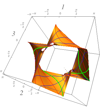
Figure 4. A slice $\pi_{+}(\pi_{-}^{-1}(v))$ of the scattering surface.

Fix the itinerary to be $\Delta_{12}\Delta_{13}$: first 1 and 2 collide, then 1 and 3. We will explore a small part of the corresponding translation-reduced scattering relation ${\mathcal{R}}={\mathcal{R}}(\Delta_{12}\Delta_{23})$. The space of lines in $\mathbb{R}^{4}$ being 6 dimensional, ${\mathcal{R}}$ forms a 6-dimensional Lagrangian relation, so a 6-dimensional submanifold of $T^{*}S^{3}\times T^{*}S^{3}$.We will fix the incoming direction $v_{-}$ of the incoming ray $\ell_{-}$ but we leave the “impact parameter’ $Q_{-}$ free. For specificity, let us fix the incoming direction $v_{-}\in E_{v}$ by supposing that the three masses come in from infinity with their directions equally spaced to form the vertices of an equilateral triangle: $(v_{1-},v_{2-},v_{3-})=(1,exp(2\pi i/3),exp(4\pi i/3)$. (Take the equal masses to be $m_{1}=m_{2}=m_{3}=1/3$ so that $v_{-}$ is unit length.) We computed all possible outgoing velocities $v_{+}=(v_{1}^{+},v_{2}^{+},v_{3}^{+})$. The results are depicted in 4. These outgoing velocities form a 2-dimensional surface within the 3-sphere $S(E_{v})$ of all possible unit length velocities in $E$. We have coordinatized this surface by projecting $v_{+}$ to its three component vectors $v_{i}^{+}\in\mathbb{C}$ and then plotting the argument of that complex number.

As described in theorem 5, the quotient of ${\mathcal{R}}$ by scaling forms a 5-dimensional Legendrian submanifold ${\mathcal{R}}/\mathbb{R}^{+}$ inside the projectivized cotangent bundle of the product of our incoming and outgoing velocity spheres. The Legendrian map $\pi_{-}\times\pi_{+}$ of theorem 5 takes the relation onto a 5 dimensional hypersurface (probably with singularities) within the product of the incoming and outgoing velocity 3-spheres By freezing the value of $v_{-}$ we have depicted in figure 4 a single two-dimensional ‘slice’ of this hypersurface, namely the surface $\pi_{+}(\pi_{-}^{-1}(v_{-}))$.

Here are details of the computation leading to the figure. After the 1st collision of 1 with 2, the 3rd particle’s velocity is unchanged. Write $v^{m}=(v_{1}^{m},v_{2}^{m},v_{3}^{m})$ for this intermediary velocity, between $\Delta_{12}$ and $\Delta_{23}$. Then $v_{3}^{m}=v_{3}^{-}$ and there is a vector $w\in\mathbb{R}^{2}$ such that $v_{1}^{m}={\textstyle\frac{1}{2}}(v_{1}^{-}+v_{2}^{-})+w$, $v_{2}^{m}={\textstyle\frac{1}{2}}(v_{1}^{-}+v_{2}^{-})-w$ with $|w|={\textstyle\frac{1}{2}}|v_{1}^{-}-v_{2}^{-}|=\frac{3}{2}$ and the direction of $w$ arbitrary.

After collision of particle number 1 and 3, we get our final velocity $v^{+}=(v_{1}^{+},v_{2}^{+},v_{3}^{+})$ with $v_{2}^{+}=v_{2}^{m}$, $v_{1}^{+}={\textstyle\frac{1}{2}}(v_{1}^{m}+v_{3}^{m})+u$, $v_{3}^{+}={\textstyle\frac{1}{2}}(v_{1}^{m}+v_{3}^{m})-u$ with $|u|={\textstyle\frac{1}{2}}|v_{3}^{m}-v_{1}^{m}|$. Use $v_{1}+v_{2}+v_{3}=0$ so that $v_{1}^{m}=-{\textstyle\frac{1}{2}}v_{3}^{-}+w$ to rewrite $v_{3}^{m}-v_{1}^{m}=\frac{3}{2}v_{3}^{-}-w$ so that $|u|=|\frac{3}{2}v_{3}^{-}-w|$.

9. Open Problems

9.1. On the closure of the Lagrangian relations.

Question 1. What are the closures of the Lagrangian relations of theorem 1?

Recall that these relations are denoted ${\mathcal{B}}(L_{1}\ldots L_{k})$ where $L_{1}L_{2}\ldots L_{k}$ is the itinerary.

Example 5.

Let us suppose the codimension $d>1$ and that ${\mathcal{B}}(L_{1}L_{2})\neq\emptyset$. Then it must be that ${\mathcal{B}}(L_{1})\neq\emptyset$ and moreover ${\rm cl}({\mathcal{B}}(L_{1}))\cap{\mathcal{B}}(L_{1}L_{2})\neq\emptyset$. For suppose that $q\in{\mathcal{B}}(L_{1}L_{2})$. Then $q$ has an edge $q_{1}q_{2}$ joining $L_{1}$ to $L_{2}$. We can perturb the endpoint $q_{2}$ slightly, off into $E$, and insure that the resulting ray $\overrightarrow{q_{1}q_{2}}$ never intersect $C$ again.

Question 2. What algebraic or combinatorial relationships hold between our Lagrangian relations?

Lagrangian relations are built to be composed. (See for example [GS] on composing linear Lagrangian relations.) How and when can we compose our Lagrangian relations? Concatenation of polygonal paths suggests that their should be some type of composition law

$${\mathcal{B}}(L_{1}L_{2}\ldots L_{k})\times{\mathcal{B}}(L_{k_{1}}L_{k+2}L_{k+s})\to^{?}{\mathcal{B}}(L_{1}L_{2}\ldots L_{k}L_{k+1}\ldots L_{k+s})$$

This “law” is nonsense if taken literally. Indeed it is doomed to failure by the background theorem, theorem 1.2.1 which implies that concatenations between relations cannot be arbitrarily long for their target is then empty.

It seems there does exist, however, some kind of “decomposition”. Write $I=L_{1}L_{2}\ldots L_{1}L_{2}\ldots L_{k},J=L_{k+1}\ldots L_{k+s}$ for two itineraries. Suppose we have a path $q\in{\mathcal{B}}(IJ)$. Moving forward in time along $q$, at each collision point $q_{i}\in L_{i}$ we have a continuous choice of new outgoing directions. In particular, at the $k$th step we could make this choice so that the new outgoing ray never intersects $C$ again. In this way we would achieve, by perturbing $q$ at the $k$th collision, a $\tilde{q}\in{\mathcal{B}}(L_{1}\ldots L_{k})$. Thus there appears to be a well-defined map: $\pi:{\mathcal{B}}(IJ)\times U\to{\mathcal{B}}(I)$ where $U$ are ‘perturbation parameters” describing how we perturbed the final outgoing ray from $L_{k}$ so as to sail off to infinity. Presumably $U\subset S^{d-1}$. Viewing this same perturbation ‘process” backwards in time, we could vary the incoming direction to $L_{k}$ at $q_{k}$ to arrive at a $\tilde{q}_{-}\in{\mathcal{B}}(J)$, and so arrive at a ‘decomposition map” ${\mathcal{B}}(IJ)\times\tilde{U}\to{\mathcal{B}}(I)\times{\mathcal{B}}(J)$.

SUBQUESTION: Is there a well-defined decomposition “morphism” ${\mathcal{B}}(IJ)\to{\mathcal{B}}(I)\times{\mathcal{B}}(J)$ ?

QUESTION 3. List all the possible itineraries $I$ with nonempty realizations ${\mathcal{B}}(I)$?

We know by the background theorem 1.2.1 that this list is finite. This last question seems to be the simplest, hardest question we have asked so far.

Acknowledgement 1.

RM would like to thank Alan Weinstein for early interest in this work, Mikhail Kapovich for discussions of CAT(0), and Bruno Nachtergaele for a crucial question leading to the section on conservation laws. RM thankfully acknowledges support by NSF grant DMS-20030177.

References

- [Arnold] V.I. Arnol’d, Mathematical Methods in Celestial Mechanics, Graduate Texts in Mathematics, 60, Springer-Verlag, 2nd edition, 1989.
- [BFK1] D. Burago, S. Ferleger and A. Kononenko, Uniform estimates on the number of collisions in semi-dispersing billiards. Annals of Mathematics 147 (1998), 695–708
- [BFK2] D. Burago, S. Ferleger and A. Kononenko, A geometric approach to semi-dispersing billiards (Survey). Ergodic Theory and Dynamical Systems 18, (1998), 303–319
- [BBI] D. Burago, Y. Burago, S. Ivanov, A course in metric geometry. Graduate Studies in Mathematics, 33. American Mathematical Society, Providence, RI, 2001.
- [DG] J. Dereziński, C. Gérard: Scattering Theory of Classical and Quantum -Particle Systems. Texts and Monographs in Physics. Berlin: Springer 1997
- [Gal] G. Galperin, Playing pool with (the number from a billiard point of view) Regular and Chaotic Dynamics, 8 No. 4 , (2003), 375–394.
- [GS] V. Guillemin, S. Sternberg, The moment map revisited. J. Diff. Geom. 69, no. 1 (2005), 137 162.
- [Hor1] L. Hörmander, Fourier integral operators I. Acta Math. 127 (1971), 79–183.
- [Hor2] L. Hörmander, The analysis of linear partial differential operators, vol. IV. Springer (1984)
- [LiMa] P. Libermann, Ch.-M. Marle, Symplectic Geometry and Analytical Mechanics. Dordrecht: Reidel, 1987
- [McG] R. McGehee, Triple Collision in the Collinear Three-Body Problem. Inventiones mathematicae 27 (1974), 191–227.
- [Mont] R. Montgomery, Infinitely many syzygies, Archives for Rational Mechanics and Analysis, v. 164, no. 4, 311-340, 2002.