A Fundamental Line of Black Hole Activity

Abstract

Black hole systems with outflows are characterized by intrinsic physical quantities such as the outflow beam power, $L_{j}$, the bolometric accretion disk luminosity, $L_{bol}$, and black hole mass or Eddington luminosity, $L_{Edd}$. When these systems produce compact radio emission and X-ray emission, they can be placed on the fundamental plane (FP), an empirical relationship between compact radio luminosity, X-ray luminosity, and black hole mass. We consider a fundamental line (FL) of black hole activity written in terms of dimensionless intrinsic physical quantities: $\rm{log}(L_{j}/L_{Edd})=A~{}\rm{log}(L_{bol}/L_{Edd})+B$ or equivalently $\rm{log}(L_{j}/L_{bol})=(A-1)~{}\rm{log}(L_{bol}/L_{Edd})+B$, and show that the FP may be written in the form of the FL. The FL has a smaller dispersion than the FP suggesting the FP derives from the FL. Disk-dominated and jet-dominated systems have consistent best fit FL parameters suggesting they are governed by the same physics. There are sharp cutoffs at $L_{bol}/L_{Edd}\simeq 1$ and $L_{j}/L_{Edd}\simeq 0.2$, and no indication of a strong break as $L_{bol}/L_{Edd}\rightarrow 1$. Consistent values of $A$ are obtained for numerous samples including FRII sources, LINERS, AGNs with compact radio emission, and Galactic black holes, which indicate a weighted mean value of $A\simeq 0.45\pm 0.01$. The results suggest that a common physical mechanism related to the dimensionless bolometric luminosity of the disk controls the jet power relative to the disk power. The beam power $L_{j}$ can be obtained by combining FP best-fit parameters and compact radio luminosity for sources that fall on the FP.

1 Introduction

The fundamental plane (FP) of black hole activity was introduced and studied extensively by Merloni, Heinz, & Di Matteo (2003) and Falcke, Körding, & Markoff (2004). Subsequently, the FP has been studied with additional sources by many groups including Körding, Falcke, & Corbel (2006), Gültekin et al. (2009), Bonchi et al. (2013), Saikia, Körding, & Falcke (2015), and Nisbet & Best (2016), hereafter NB16. The FP encapsulates the relationship between compact radio luminosity, X-ray luminosity, and black hole mass for black hole systems and provides a good description of the data over a very large range of black hole mass. As has been discussed by many authors, such as Heinz & Sunyaev (2003), Merloni et al. (2003), Falcke et al. (2004), Körding, Fender, & Migliari (2006), Merloni & Heinz (2007), Fender (2010), de Gasperin et al. (2011), and Saikia, Körding, & Falcke (2015), to name a few, the radio luminosity, $L_{R}$, obtained by combining the radio flux density and the radio frequency, is likely to be related to the beam power or luminosity in directed kinetic energy powering the outflow, $L_{j}$. And, the X-ray luminosity, $L_{X}$, is likely to be related to the bolometric luminosity, $L_{bol}$ of the accretion disk. The relationships frequently discussed in the literature including the papers noted above are $L_{j}\propto L_{R}^{\alpha}$, where the beam power of the outflow is defined as the energy per unit time, $L_{j}\equiv dE/dt$, ejected by the source in the form of kinetic energy, and $L_{bol}\propto L_{X}(2-10\hbox{ keV})$. In addition, Saikia et al. (2015) introduce the bolometric FP that replaces $L_{X}$ with $L_{bol}$ where $L_{bol}$ is obtained from the OIII luminosity of sources. This allows sources with accretion disk luminosities determined with tracers other than X-ray luminosity to be placed on the fundamental plane.

It is important to understand the relationship between the intrinsic physical variables that describe black hole systems to determine whether they are all governed by the same physics or whether there are a variety of mechanisms that produce collimated outflows. As discussed above, given that many different types of sources with outflows fall on the FP and that the FP covers such a broad range of black hole mass, it is expected that the underlying physics governing the properties of the sources is similar. However, the precise relationship between the underlying intrinsic source parameters and empirically determined FP parameters has not been fully characterized. Here, we suggest an ansatz that allows a determination of the connection between the underlying intrinsic source quantities ($L_{j}$, $L_{bol}$, and $L_{Edd}$), and the quantities used to define the FP ($L_{R}$, $L_{X}$, and black hole mass). This also allows the relationships between intrinsic physical variables to be obtained and studied, and compared with model preditions, which are typically cast in terms of intrinsic source quantities. This ansatz is presented in section 2.

In addition, many black hole systems have empirical estimates of the bolometric accretion disk luminosity obtained with tracers other than X-ray emission or beam power estimates obtained with tracers other than compact radio emission, and thus can not be placed directly on the FP. For these sources, it is important to compare their properties with those of sources on the FP to determine whether they are governed by similar or different physical mechanisms. Such a comparison has important implications for the physics of the outflows and the accretion disk properties relative to the black hole masses for different types of sources. To determine whether the relationship between outflow properties, accretion disk properties, and black hole mass or Eddington luminosity are consistent with those indicated by the FP, it is helpful to see if the FP may be rewritten in terms of other quantities such as Eddington normalized beam power and Eddington normalized bolometric luminosity. The fact that the FP is valid over a very large black hole mass range suggests that it can be written in terms of these dimensionless luminosities. With this representation, more sources can be compared, and the range of values of dimensionless beam power and dimensionless bolometric luminosity and the relationship between these quantities can be studied. In section 2, it is shown that the FP is likely the empirical manifestation of an underlying relationship between the dimensionless beam power and dimensionless bolometric accretion disk luminosity. Applications to data sets are presented in section 3. The results and implications are discussed in section 4, and summarized in section 5.

2 Analysis

The FP may be written in the form of eq. (1), where the units and precise definitions of $L_{R}$, $L_{X}$, and $M$ vary from paper to paper, and a, b, and c are empirically determined constants. Using the different definitions of $L_{R}$, $L_{X}$, and the black hole mass $M$ in each paper, it is possible to convert these definitions to a common scale, which was done by NB16. Here, we follow the definitions presented by NB16:

$$\rm{log}~{}L_{R}=a~{}\rm{log}~{}L_{X,42}+b~{}\rm{log}~{}M_{8}+c~{},$$ (1)

where $L_{R}$ is the 1.4 GHz radio power of the compact radio source in $\hbox{erg s}^{-1}$, $L_{X,42}$ is the (2 - 10) keV X-ray luminosity of the source in units of $10^{42}\hbox{ erg s}^{-1}$, and $M_{8}$ is the black hole mass in units of $10^{8}M_{\odot}$; conversions to and from other wavebands are discussed by NB16. NB16 present results obtained with a sample of 576 LINERS and summarized the results of Merloni et al. (2003), Körding et al. (2006), Gültekin et al. (2009), Bonchi et al. (2013), and Saikia et al. (2015).

Sources with a huge range of black hole mass, about nine orders of magnitude, follow the functional form of eq. (1), suggesting that the relationship between the intrinsic physical quantities $L_{j}$, $L_{bol}$, and black hole mass $M$ (or $L_{Edd}$) scale in such a way that the overall relationship is maintained. If the equation that describes the relationship between intrinsic physical variables is written in terms of dimensionless quantities then it is scale-invariant and we expect the relationship between intrinsic variables to remain valid for all scales. The simplest equation written in terms of dimensionless quantities with a form similar to that of the fundamental plane is

$$\rm{log}\left({L_{j}\over L_{Edd}}\right)=A~{}\rm{log}\left({L_{bol}\over L_{Edd}}\right)+B,$$ (2)

where $L_{Edd}$ is the Eddington luminosity, $L_{Edd}\simeq 1.3\times 10^{46}M_{8}~{}\hbox{erg s}^{-1}$, and $A$ and $B$ are constants. So, the goal is to determine whether eq. (1) can be written in the dimensionless and Eddington-normalized form of eq. (2).

As described in section I, it is convenient to write the bolometric luminosity of the accretion disk as

$$L_{bol}=\kappa_{X}~{}L_{X}(2-10\hbox{ keV})$$ (3)

where $\kappa_{X}$ is a constant, and the beam power $L_{j}$ as

$$\rm{log}L_{j}=C~{}\rm{log}~{}L_{R}+D~{},$$ (4)

where $C$ and $D$ are constants, and $L_{bol}$, $L_{X}(2-10\hbox{ keV})$, $L_{j}$, $L_{R}$, and $L_{Edd}$ have units of $\hbox{erg s}^{-1}$. Substituting eqs. (3) and (4) into eq. (1) indicates that

$$\rm{log}\left({L_{j}\over L_{Edd}}\right)=aC~{}\rm{log}L_{bol}-(1-bC)~{}\rm{log}L_{Edd}+\kappa$$ (5)

where $\kappa=D+C(c-42~{}a-46.11~{}b-a~{}\rm{log}\kappa_{X})$.

Eq. (5) may be written in the form of eq. (2) when $aC=(1-bC)$; that is, when $C=(a+b)^{-1}$. Thus, if it turns out that $C=(a+b)^{-1}$ then the FP, given by eq. (1), may be rewritten in the mass-scale-invariant form given by eq. (2). In this case, it is easy to show that $A=a/(a+b)$ and $B=\kappa$.

Three approaches are used to determine whether the value of $C$ is equal to $(a+b)^{-1}$. First, $C$ is computed using $C=(a+b)^{-1}$, and the values obtained for different data sets are shown to be consistent. The values are compared with those indicated by independent theoretical studies and independent studies of radio sources, and it is shown that there is good agreement between the empirical values, $C=(a+b)^{-1}$, theoretically predicted values, and values based on independent studies of radio sources. Second, the values of $aC$ and $(1-bC)$ are computed using the value of $C$ indicated by independent theoretical studies and independent studies of radio sources, and the difference between $aC$ and $(1-bC)$ is shown to be consistent with zero. And, third, again using the value of $C$ indicated by independent theoretical studies and independent studies of radio sources, the ratio of $aC$ to $(1-bC)$ is computed and is shown to be consistent with unity. These results indicate that $aC$ is equal to $(1-bC)$, thus $C$ does equal $(a+b)^{-1}$, implying that eq. (1) may be written in the form of eq. (2). Details of the three analyses just described are presented in section 2.1 and are summarized in section 2.2.

Table 1: Study of the Parameters Discussed in Section 2

(1)	(2)	(3)	(4)	(5)	(6)	(7)	(8)	(9)
Sample	$C={1\over(a+b)}$	$aC$	$(1-bC)$	$aC-(1-bC)$	${aC\over(1-bC)}$	$A={a\over(a+b)}$	$B=\kappa$	$D$
NB16(1)	$0.75\pm 0.07$	$0.46\pm 0.05$	$0.51\pm 0.07$	$-0.05\pm 0.09$	$0.90\pm 0.18$	$0.49\pm 0.05$	$-1.87\pm 2.09$	$14.93\pm 2.61$
M03	$0.72\pm 0.08$	$0.43\pm 0.08$	$0.45\pm 0.07$	$-0.02\pm 0.11$	$0.95\pm 0.25$	$0.43\pm 0.05$	$-2.80\pm 1.99$	$15.86\pm 3$
K06	$0.72\pm 0.26$	$0.45\pm 0.28$	$0.47\pm 0.21$	$-0.02\pm 0.36$	$0.96\pm 0.75$	$0.46\pm 0.19$	$-2.70\pm 2.03$	$15.76\pm 10.1$
K06	$0.74\pm 0.11$	$0.40\pm 0.05$	$0.45\pm 0.13$	$-0.04\pm 0.14$	$0.91\pm 0.30$	$0.42\pm 0.06$	$-2.52\pm 1.96$	$15.58\pm 4.03$
G09	$0.69\pm 0.14$	$0.48\pm 0.09$	$0.45\pm 0.19$	$0.03\pm 0.21$	$1.07\pm 0.51$	$0.46\pm 0.10$	$-3.90\pm 2.04$	$16.96\pm 5.43$
G09	$0.69\pm 0.06$	$0.44\pm 0.07$	$0.42\pm 0.06$	$0.02\pm 0.09$	$1.05\pm 0.25$	$0.43\pm 0.05$	$-3.88\pm 1.98$	$16.94\pm 2.38$
B13	$0.93\pm na$	$0.28\pm 0.04$	$0.52\pm na$	$-0.24\pm na$	$0.54\pm na$	$0.36\pm na$	$5.07\pm 1.86$	$7.99\pm na$
S15	$0.80\pm 0.29$	$0.45\pm 0.28$	$0.57\pm 0.14$	$-0.11\pm 0.32$	$0.80\pm 0.54$	$0.51\pm 0.18$	$na\pm na$	$na\pm na$
S15	$0.61\pm 0.13$	$0.59\pm 0.21$	$0.42\pm 0.14$	$0.17\pm 0.26$	$1.41\pm 0.71$	$0.50\pm 0.11$	$-7.58\pm 2.11$	$20.64\pm 5$

2.1 Details of the Analysis

The values of $C=1/(a+b)$ are listed in Table 1 for the values of $a$ and $b$ summarized in Table 3 of NB16. The nine values of $C$ obtained are all consistent; they range from about 0.61 to 0.93 with a median value of 0.72 and unweighted mean value of $0.74$; all of the sources are within one sigma of these mean and median values, as expected based on the consistency of the values of $a$ and $b$ listed by NB16. As discussed below, the mean and median values of $C$ are consistent with theoretical predictions and independent studies of radio sources.

Theoretical studies such as those by Heinz & Sunyaev (2003) and Merloni & Heinz (2007) indicate that the value of $C$ is expected to be $12/17\simeq 0.71$ when the radio spectral index of the compact radio source is close to zero and the radio emission is not affected by Doppler beaming and boosting due to bulk motion. This agrees with the value of $0.71\pm 0.03$ indicated by the independent studies of radio sources, discussed below. The fact that the values of $C$ indicated by the best fit values of $a$ and $b$ (see column 2 of Table 1) are consistent with that predicted theoretically and indicated by independent studies of radio sources suggests that relativistic beaming is likely to have a small effect on the compact radio emission for most of the sources used to construct the fundamental plane.

An independent estimate of $C$, and an independent estimate of $D$, may be obtained by considering independent studies of radio sources. Using the empirically determined relation between core radio luminosity and extended radio luminosity for radio galaxies presented by Yuan & Wang (2012) and applying the conversion of extended radio luminosity to beam power presented by Willott et al. (1999), we obtain $C=0.71\pm 0.03$ and $D=14.2\pm 1.0$. Note that this is only used to confirm in general terms that $C$ is consistent with $(a+b)^{-1}\simeq 0.7$; the results of Willott et al. (1999) are not used to compute the beam power for any of the sources presented in this paper.

To further test whether eq. (5) can be written in the form of eq. (2), the values of $aC$ and $(1-bC)$ and their difference and ratio are computed and listed in columns (3), (4), (5), and (6) of Table 1, where the value of $C$ indicated above of $0.71\pm 0.03$ is used to compute values for columns (3) through (6). The difference listed in column (5) is consistent with zero for all of the samples. And, the ratio $aC/(1-bC)$ listed in column (6) is consistent with unity. Thus, eq. (1) can be written in the form of eq. (2).

2.2 Summary of the Analysis

These considerations indicate that eq. (1) may be written in the form of eq. (2), where $A=a/(a+b)$, $C=1/(a+b)$, and $B=\kappa$. In terms of understanding the physics of the sources and constraining models that describe the sources, $A$ is the most important parameter since eq. (2) implies that $L_{j}\propto L_{bol}^{A}~{}M^{(1-A)}$ $\propto L_{bol}^{A}~{}L_{Edd}^{(1-A)}$. The parameter $A$ may be obtained using best fit parameters $a$ and $b$, or by fitting to the fundamental line (FL) given by eq. (2). The value of $A$ obtained from the best fit values of $a$ and $b$ are listed in column (7) of Table 1 for nine samples of sources, and all values are consistent within the uncertainties. Values of $A$ obtained from eq. (2) by fitting directly to Eddington normalized luminosities are discussed in section 3.

The y-intercept of the FL is described by $B$. The value of $B$ may be obtained from $B=\kappa$, which requires values of $C$, $D$, $\rm{log}\kappa_{X}$ as well as best fit values of $a$, $b$, and $c$. To compute $B$, the value of $C$ listed in column (2) of Table 1 is used, as is $D=14.2\pm 1.0$ obtained as described above. To obtain an estimate for $\rm{log}\kappa_{X}$, the bolometric luminosity of each source with a measured (2-10 keV) X-ray luminosity listed by Merloni et al. (2003) was obtained using eq. (21) from Marconi et al. (2004); this indicates a mean value of $\rm{log}\kappa_{X}=1.18\pm 0.03$, or $\kappa_{X}\simeq 15.1$, which is in good agreement with the value obtained by Ho (2009). It is easy to show that propagating the uncertainties of all parameters, the uncertainty of $c$ has an insignificant impact on the uncertainty of $B$, so this term is not included in computing the uncertainty of $B$. With these values, $B$ is obtained and listed in column (8) of Table 1.

In addition, we may write $D=B-C(c-42~{}a-46.11~{}b-a~{}\rm{log}\kappa_{X})$ so that a value of $D$ may be obtained for each sample if an estimate of the value of $B$ is available, given the value $\rm{log}\kappa_{X}$ described above and the value of $C$ listed in column (2) of Table 1. Daly (2016) studied a sample of 97 FRII AGN for which beam powers, bolometric luminosities, and Eddington luminosities were available and fitting to eq. (6) obtained a value of $B=-1.14\pm 0.06$. Values of $D$ obtained with this value of $B$ are listed in column (9) of Table 1. It is easy to show that propagating the uncertainties of all parameters, the uncertainty of $c$ has an insignificant impact on the uncertainty of $D$, so this term is not included in computing the uncertainty of $D$.

Table 2: Best-fit Parameters to Eq. (2), as Described in Section 3

(1)	(2)	(3)	(4)	(5)	(6)
Sample	N	A	B	Dispersion of FL	Dispersion of FP
NB16	576 LINERS	$0.43\pm 0.02$	$-1.08\pm 0.08$	0.47	0.73
M03	80 AGN + 36 GBH	$0.45\pm 0.03$	$-0.94\pm 0.10$	0.65	0.88
M03	80 AGN	$0.41\pm 0.04$	$-1.34\pm 0.14$	0.71
D16	97 FRII AGN	$0.44\pm 0.05$	$-1.14\pm 0.06$	0.38
S15	102 GBH	$0.47\pm 0.02$	$-1.37\pm 0.04$	0.19
S15	102 GBH ($\kappa_{X}=5$)	$0.47\pm 0.02$	$-1.15\pm 0.04$	0.19
Combined Sample	855 sources	$0.41\pm 0.01$	$-1.19\pm 0.04$	0.47
Combined Sample	855 sources	$0.39\pm 0.01$	$-1.27\pm 0.04$	0.48

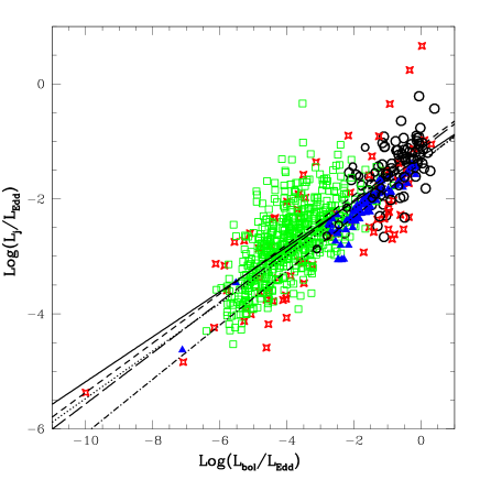
Figure 1: The log of the Eddington normalized beam power is shown versus the log of the Eddington normalized bolometric accretion disk luminosity for 576 LINERS (open green squares), 80 AGN (open red stars), 102 GBH measurements (solid blue triangles), and 97 powerful extended radio sources (open black circles); values of quantities are obtained as described in Section 3. The best fit lines are: medium dashed line (576 LINERS); dotted line (80 AGN); dot-dash line (102 GBH); long-dashed line (97 FRII AGN); and solid line (all 855 measurements). These symbols are used throughout the paper. Best fit parameters to eq. (2) for the quantities shown here are listed in Table 2 and discussed in Section 3.

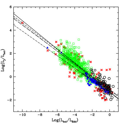
Figure 2: The log of the ratio of beam power to bolometric accretion disk luminosity is shown versus the log of the Eddington normalized bolometric luminosity for the sources shown in Fig. 1. See eq. (6) and the discussion in section 4.

3 Applications

The FL, given by eq. (2) or (6), may be studied when values of $L_{j}$, $L_{bol}$, and $L_{Edd}$ are available for sources. There are numerous well-studied methods to estimate the latter two, but there are only a few methods to estimate $L_{j}$. The results presented in section 2 indicate that the beam power $L_{j}$ may be obtained using eq. (4) for sources that lie on the FP and have best-fit FP parameters a, b, and c determined, since both $C$ and $D$ in eq. (4) depend upon the best-fit FP for that type of source. That is, each type of source may have different best fit FP parameters and hence different values of $C$ and $D$; once the best fit FP parameters are determined for that type of source, eq. (4) may be used to solve for the beam power of individual sources of that type. For example, given the source types compiled and studied by NB16, the value of $C$ is listed in column 2, and that of $D$ is listed in column 9 of Table 1. In addition, there are many types of sources that have beam power determinations that do not have compact radio emission and hence can not be placed on the FP. For example, O’Dea et al. (2009) used multi-frequency radio images to determine the beam power of powerful classical double (FRII) radio sources by applying the equations of strong shock physics and showed that this method allows a determination of the beam power that is very insensitive to assumptions. Notably, the beam power obtained does not depend upon assumptions related to the distribution of energy between relativistic particles and magnetic fields since the offsets from minimum energy conditions cancel out when the beam power is written in terms of empirically determined quantities. Results obtained for FRII sources for which values of $Lj$ were obtained using this method will be discussed below, and the results of fits to eqs. (2) and (6) are described in detail by Daly (2016).

To obtain and study $L_{j}/L_{Edd}$ and $L_{bol}/L_{Edd}$ for sources with best fit FP parameters, samples were selected from the list of NB16 in such a way as to avoid duplicate measurements of any given source while maintaining the integrity of each sample. That is, some sources are common to different samples, and rather than removing sources from samples, representative samples were selected such that the samples do not have observations in common. The samples considered include the 576 LINERS presented by NB16, the 80 AGNs, which are all compact radio sources, presented by Merloni et al. (2003), and the 102 measurements of Galactic black holes (GBH) that are X-ray binaries presented by Saikia et al. (2015). The value of $L_{bol}$ is obtained for each source using eq. (3) with the value of $\rm{log}~{}\kappa_{X}$ described above (one additional value is considered for the GBH), black hole mass is converted to $L_{Edd}$ with the relation listed above, and $L_{j}$ is obtained using eq. (4) given the values of $C$ and $D$ listed in columns (2) and (9) of Table 1. A value of $D$ is not available for the Saikia et al. (2015) fit that included GBH (see row 8 of Table 1), but the fit of NB16(1) has values of $a$ and $b$ that are consistent with those of Saikia et al. (2015) and this fit goes right through the GBH points, so the NB16(1) values of $C$ and $D$ are applied to that sample; in addition, a value of $\kappa_{X}=5$ suggested by Saikia et al. (2015) is also considered for the GBH. All values of $L_{R}$ are scaled to 1.4 GHz using the conversion factors of NB16. In addition, 97 FRII AGN from Daly (2016) are included; independent values of $L_{j}$, $L_{bol}$, and $L_{Edd}$ are available for these sources. These samples allow a comparison between sources of various types.

Results obtained with these four samples and the combined sample are shown in Fig. 1 and are summarized in Table 2; the results shown in Fig. 1 are obtained for $\rm{log}\kappa_{X}=1.18\pm 0.03$ (i.e. $\kappa_{X}\simeq 15.1$) for all sources, and the values of $L_{bol}$ decrease by about a factor of 3 for the GBH for $\kappa_{X}\simeq 5$. All fits are unweighted. To estimate the dispersion of $y=\rm{log}(L_{j}/L_{Edd})$, $\sigma_{y}$, we assume that all of the dispersion in the fit is due to the uncertainty in $y$, and following Merloni et al. (2003) and Gültekin et al. (2009), we assume the uncertainty is the same for each point. Setting the reduced $\chi^{2}$ to unity then provides an estimate of $\sigma_{y}$. If there are additional sources of error, such as errors in $x=\rm{log}(L_{bol}/L_{Edd})$, then $\sigma_{y}$ will decrease since the total dispersion $\sigma_{T}^{2}=\sigma_{y}^{2}+\sigma_{x}^{2}$. For example, if $\sigma_{x}=\sigma_{y}$, then the dispersion will decrease by a factor of $1/\sqrt{2}$ from the values listed in column (5) of Table 2.

The values of the dispersion of the FL listed in column (5) of Table 2 can be compared with values of the dispersion of the FP, which are available for two of the samples studied, and these are listed in column (6) of Table 2. The fundamental line (FL) described by eq. (2) has a smaller dispersion than the FP. This is another indication that eq. (2) provides a good description of the data. Indeed, it suggests that the FL, which is closely tied to intrinsic source properties, leads to the FP, which is closely tied to empirical source properties. That is, it suggests that the FP derives from or is the result of the FL.

The results presented in Table 2 for the combined sample support the idea (Saikia et al. 2015) that the conversion factor $\kappa_{X}$ is about three times larger for AGN than it is for GBH since the dispersion of the combined sample is a bit smaller when the value of $\kappa_{X}$ is larger for AGN than it is for GBH.

Fig. 1 indicates that eq. (2) provides a good description of the data over about 10 orders of magnitude in $L_{bol}/L_{Edd}$, from about $10^{-10}$ to about $1$, and over about 5 orders of magnitude in $L_{j}/L_{Edd}$, from about $10^{-5.5}$ to about $0.3$. Interestingly, the relationship seems to remain valid all the way up to values of $L_{bol}/L_{Edd}\rightarrow 1$. Within uncertainties, the relationship between the dimensionless parameters indicated by the FL is the same for all types of sources studied including LINERS, AGNs that are compact radio sources, GBH, and FRII AGNs. In addition, the values of $A$ indicated by best-fit fundamental plane parameters a and b, listed in column (7) of Table 1, are consistent with those obtained by a direct fit to the data, listed in Table 2.

4 Discussion

The FL, given by equation (2), may be re-written as

$$\rm{log}\left({L_{j}\over L_{bol}}\right)=(A-1)~{}\rm{log}\left({L_{bol}\over L_{Edd}}\right)+B.$$ (6)

This may be interpreted as the efficiency of the beam power relative to accretion disk power as a function of Eddington normalized disk luminosity. It is interesting to consider the range of values of this parameter, and results obtained with the samples discussed above are shown in Fig. 2. Here $y=\rm{log}(L_{j}/L_{bol})$, and the dispersion of this parameter for each sample and for the combined sample is the same as those quoted in Table 2 for $y=\rm{log}(L_{j}/L_{Edd})$; best fit values of the slope $(A-1)$, shown in Fig. 2, can easily be obtained from the values of $A$ listed in Table 2.

Values of $L_{j}/L_{bol}$ extend over about 7 orders of magnitude from about $10^{-2}-10^{5}$, and the relationship between $L_{j}/L_{bol}$ and $L_{bol}/L_{Edd}$ is similar for all classes of objects studied.

The transition from sources with $L_{j}>L_{bol}$, considered to be “jet dominated,” to those with $L_{j}<L_{bol}$, considered to be “disk dominated,” occurs at about $L_{bol}/L_{Edd}\sim 10^{-2}$, which agrees with the results obtained by Best & Heckman (2012) and NB16. This is consistent with previous results that find that “jet dominated” sources have low values of $L_{bol}/L_{Edd}$, while those that are “disk dominated” have high values of this parameter (e.g. see the summaries of Fender 2010; Best & Heckman (2012); Heckman & Best 2014; Yuan & Narayan 2014; and NB16).

There is no change or break in the relationship between the ratio $L_{j}/L_{bol}$ and $L_{bol}/L_{Edd}$ at $L_{j}/L_{bol}\sim 1$; that is sources with $L_{j}/L_{bol}<1$ and those with $L_{j}/L_{bol}>1$ have the same relationship between $L_{j}/L_{bol}$ and $L_{bol}/L_{Edd}$. This indicates that there is little or no difference between the physics of “disk dominated” and “jet dominated” sources for the types of radio loud sources studied here. These results suggest that they are governed by the same physics and are described by the same equations.

As noted above, there appears to be a rather sharp cut-off of sources at $L_{bol}/L_{Edd}\sim 1$ indicating that sources with outflows that fall on the FP and FL do not have super-Eddington luminosities. In addition, there does not seem to be a strong change in the relationship between $L_{j}/L_{bol}$ and $L_{bol}/L_{Edd}$ as $L_{bol}/L_{Edd}\rightarrow 1$.

The relationship obtained between $L_{j}/L_{bol}$ and $L_{bol}/L_{Edd}$ for the FRII AGN studied by Daly (2016) is the same as that obtained here for many other types of sources. Daly (2016) showed that this relationship is consistent with models in which the outflow is powered by the spin of the black hole, such as the Blandford-Znajek mechanism (Blandford & Znajek 1977). The same reasoning applies here, which implies that outflows from the other types of systems studied here, including LINERS, AGNs that are compact radio sources, and GBH have outflow and disk properties that are also consistent with models in which the outflow is powered by the spin of the black hole. That is, the value of $A$ obtained here is consistent with predictions in models with $L_{bol}\propto\epsilon~{}\dot{M}\propto\epsilon~{}\dot{m}~{}M$, and $L_{j}\propto\dot{m}~{}M~{}f(j)$, where $\dot{M}$ is the mass accretion rate, $\dot{m}\equiv\dot{M}/\dot{M}_{Edd}$ is the dimensionless mass accretion rate, $\dot{M}_{Edd}\equiv L_{Edd}c^{-2}$ is the Eddington accretion rate, $\epsilon$ is a dimensionless efficiency factor, and $f(j)$ is a function of black hole spin (see Daly 2016). These equations imply that for a value of $A$ of 0.5, $\epsilon\propto\dot{m}$, and for a value of $A$ of 0.45, $\epsilon\propto\dot{m}^{1.2}$ (see Daly 2016 for a detailed discussion). The equation for $L_{j}$ is that expected in the Blandford-Znajek (1977) model of spin energy extraction if the magnetic field $B$ is given by $B^{2}\propto(\dot{m}/M)$, and this is expected to be the case for several types of accretion disks, such as ADAF and MAD accretion disks (e.g. Tchekhovskoy et al. 2010; Yuan & Narayan 2014). Note that these results are consistent with those obtained by Fender, Gallo, & Jonker (2003), who find $L_{j}\propto L_{X}^{0.5}$.

Even though the maximum value of $L_{bol}/L_{Edd}$ is close to one, the maximum value of $L_{j}/L_{Edd}$ is about (0.1 - 0.3) (see Fig. 1). Still, this is a large value for $L_{j}/L_{Edd}$, indicating very powerful outflows relative to the Eddington luminosity. The fact that this is less than one and in the range of 0.1 to 0.3 may be related to the limit that, at most, 29 % of the mass-energy of a black hole can be due to the spin energy of the hole, so at most 29 % of the mass-energy can be extracted electromagnetically or with any other mechanism (e.g. Blandford 1990).

5 Summary

The fact that the FP is manifestly scale invariant suggests that it represents a relationship between the Eddington normalized beam power and Eddington normalized bolometric luminosity of the black hole system. In section 2 it is shown that the dimensionless representation given by eq. (2) is consistent with independent emipirical and theoretical studies of radio sources (see columns 2, 5, and 6 of Table 1). Given that eq. (1) may be written in the form of eq. (2), the value of $A$ may be written in terms of the best fit FP parameter values $a$ and $b$: $A=a/(a+b)$, and these values are listed in Table 1. Another way to determine the value of $A$ is described in section 3: the beam power $L_{j}$ of a source may be determined using eq. (4) given the values of $C$ and $D$ listed in Table 1 for sources of that type, and the value of $L_{bol}$ may be obtained using eq. (3). A direct fit to eq. (2) is then possible since it is easy to convert black hole mass to $L_{Edd}$. The values of $A$ obtained by a direct fit to the data are presented in Table 2.

In terms of understanding the physics of the sources and constraining models that describe the sources, $A$ is of paramount importance since eq. (2) implies that $L_{j}\propto L_{bol}^{A}~{}M^{(1-A)}$. All nine samples studied are consistent with a single value of $A$ and yield a mean value of $0.45\pm 0.02$ (see column (7) of Table 1); this is consistent with the value of $0.44\pm 0.05$ obtained by Daly (2016) for FRII AGN. The mean value of $A$ for the four samples that make up the “combined sample” listed in Table 2 is $0.45\pm 0.01$. However, the fit to the combined sample indicates a smaller value of $A$, which is likely due to the different y-intercepts of the samples causing offsets that modify the value of $A$ for the fit to the combined sample.

Two equivalent forms of the FL, given by eqs. (2) and (6), are studied directly using four data sets that include LINERS, AGNs that are compact radio sources, GBH, and FRII AGN. All categories of source have consistent best fit values of $A$ and $B$ (see Figs. 1 and 2 and Table 2), and the FL has a smaller dispersion than the FP, supporting the longstanding interpretation of the FP as arising from a relationship between the intrinsic physical variables that describe black hole systems. This representation allows a study of the range of values of $L_{j}/L_{Edd}$, $L_{bol}/L_{Edd}$, and $L_{j}/L_{bol}$, and the relationships between these parameters. For the sources studied $L_{j}/L_{Edd}$ ranges from about $10^{-5.5}$ to about 0.3; $L_{bol}/L_{Edd}$ ranges from about $10^{-10}$ to about 1; and $L_{j}/L_{bol}$ ranges from about $10^{-2}$ to about $10^{5}$. These results indicate that the sources transition from jet dominated to disk dominated, which is defined to occur at $L_{j}/L_{bol}\sim 1$, at a value of $L_{bol}/L_{Edd}\sim 10^{-2}$, which is consistent with the value obtained by others (e.g., Best & Heckman 2012; NB16). Interestingly, the relationships between the dimensionless parameters $L_{j}/L_{bol}$ or $L_{j}/L_{Edd}$ and $L_{bol}/L_{Edd}$ seem to remain valid over the full range of values of $L_{bol}/L_{Edd}$ studied, including $L_{bol}/L_{Edd}\sim 1$, and over the full range of values from $L_{j}/L_{bol}<<1$ to $L_{j}/L_{bol}>>1$. The values of $A$ and $B$, particularly $A$, describe the physics of the sources and have implications for models of black hole systems. The fact that one dimensionless equation, eq. (2) or eq. (6), describes all sources, including sources that do not have compact radio emission, over such large ranges of dimensionless parameters, suggests that a common physical mechanism set primarily by $L_{bol}/L_{Edd}$ regulates the beam power relative to the accretion disk power in these systems. Note that this includes the possibility that $L_{bol}/L_{Edd}$ may be impacted by $L_{j}/L_{Edd}$ through feedback mechanisms.

References

- Best & Heckman (2012) Best, P. N., & Heckman, T. M. 2012, MNRAS, 421, 1569
- Blandford (1990) Blandford, R. D. 1990, in Active Galactic Nuclei, ed. T. J. L. Courvoisier & M. Mayor (Berlin: Springer), 161
- Blandford & Znajek (1977) Blandford, R. D., & Znajek, R. L. 1977, MNRAS, 179, 433
- Bonchi et al. (2013) Bonchi A., La Franca F., Melini G., Bongiorno A., & Fiore F., 2013, MNRAS, 429, 1970
- Daly (2016) Daly, R. A. 2016, MNRAS 458, L24
- de Gasperin et al. (2011) de Gasperin, F., Merloni, A., Sell, P., Best, P., Heinz, S., & Kauffmann, G. 2011, MNRAS, 415, 2910
- Falcke et al. (2004) Falcke, H., Körding, E., & Markoff, S. 2004, A&A, 414, 895
- Fender (2010) Fender, R. 2010, in The Jet Paradigm, Lecture Notes in Physics. Springer-Verlag Berlin, 794, 115
- Fender et al. (2003) Fender, R. P., Gallo, E., & Jonker, P. G. 2003, MNRAS, 343, L99
- Gültekin et al. (2009) Gültekin K., Cackett E. M., Miller J. M., Di Matteo T., Markoff S., & Richstone D. O., 2009, ApJ, 706, 404
- Heckman & Best (2014) Heckman, T. M., & Best, P. N. 2014, ARA&A, 52, 589
- Heinz & Sunyaev (2003) Heinz S. & Sunyaev R. A., 2003, MNRAS, 343, L59
- Ho (2009) Ho, L. C. 2009, ApJ, 699, 626
- Körding et al. (2006) Körding E. G., Falcke H., & Corbel S., 2006, A&A, 456, 439
- Körding et al. (2006b) Körding, E. G., Fender, R. P., & Migliari, S. 2006, MNRAS, 369, 1451
- Marconi et al. (2004) Marconi, A., Risaliti, G., Gilli, R., Hunt, L. K., Maiolino, R., & Salvati, M. 2004, MNRAS, 351, 169
- Merloni & Heinz (2007) Merloni A. & Heinz S., 2007, MNRAS, 381, 589
- Merloni et al. (2003) Merloni A., Heinz S., & di Matteo T., 2003, MNRAS, 345, 1057
- Nisbet & Best (2016) Nisbet, D. M., & Best, P. N. 2016, MNRAS, 455, 2551
- O’Dea et al. (2009) O’Dea, C. P., Daly, R. A., Freeman, K. A., Kharb, P., & Baum, S. 2009, A&A, 494, 471
- Saikia et al. (2015) Saikia P., Körding E., & Falcke H., 2015, MNRAS, 450, 2317
- Tchekhovskoy, Narayan, & McKinney (2010) Tchekhovskoy, A., Narayan, R., McKinney, J. C. 2010, ApJ, 711, 50
- Willott et al. (1999) Willott, C. J., Rawlings, S., Blundell, K. M., & Lacy, M. 1999, MNRAS, 309, 1017
- Yuan & Narayan (2014) Yuan, F., & Narayan, R. 2014, ARA&A, 52, 529
- Yuan & Wang (2012) Yuan, Z., & Wang, J. 2012, ApJ, 744:84, 1