State Space Path Integrals for Electronically Nonadiabatic Reaction Rates

Abstract

We present a state-space-based path integral method to calculate the rate of electron transfer (ET) in multi-state, multi-electron condensed-phase processes. We employ an exact path integral in discrete electronic states and continuous Cartesian nuclear variables to obtain a transition state theory (TST) estimate to the rate. A dynamic recrossing correction to the TST rate is then obtained from real-time dynamics simulations using mean field ring polymer molecular dynamics. We employ two different reaction coordinates in our simulations and show that, despite the use of mean field dynamics, the use of an accurate dividing surface to compute TST rates allows us to achieve remarkable agreement with Fermi’s golden rule rates for nonadiabatic ET in the normal regime of Marcus theory. Further, we show that using a reaction coordinate based on electronic state populations allows us to capture the turnover in rates for ET in the Marcus inverted regime.

1 Introduction

Condensed-phase electron transfer (ET) reactions drive a wide range of energy conversion and catalytic pathways in biological systems^{1, 2, 3} and renewable energy devices.^{4, 5, 6} Developing theoretical methods capable of accurately calculating rate constants for these reactions is an ongoing challenge and a crucial step towards the design of materials with desirable charge and energy transfer properties. While numerous mixed quantum-classical ^{7, 8, 9} and semiclassical methods^{10, 11, 12, 13, 14} for simulating ET reactions in the condensed phase have been developed over the years, they are limited by either computational complexity or the use of dynamics that fail to preserve detailed balance. Alternatively, methods based on imaginary-time path integrals (PIs) such as centroid molecular dynamics (CMD)¹⁵ and ring polymer molecular dynamics (RPMD) ¹⁶ that employ classical trajectories to capture quantum dynamics effects have emerged as promising methods for the computation of condensed-phase reaction rates.^{17, 18, 19, 20} RPMD in particular has been successfully employed to study a variety of chemical reactions^{21, 22, 23, 24, 25} and was shown to accurately predict thermal rate constants for ET in the normal and activationless regimes of Marcus theory.²¹ More recently, extensions of RPMD to systems with multiple coupled electronic states have been developed;^{26, 27, 28, 29} notably, the kinetically constrained (KC)-RPMD method²⁸ accurately describes the ET reactions of two-level systems both in the normal and inverted regimes of Marcus theory.

In this paper, we present a simple and accurate method to calculate rate constants for nonadiabatic ET reactions. We first evaluate the transition state theory (TST) rate estimate using an exact state space path integral (SS-PI) to compute the probability of reaching the transition state (dividing surface) from the reactant state. The dynamic recrossing factor to correct the TST rate is then computed using mean field (MF)-RPMD,³⁰ with trajectories initialized to the dividing surface. This approach generalizes the standard RPMD implementation to multi-state, multi-electron systems with very little additional complexity and retains all the desirable features of RPMD including, most notably, the conservation of detailed balance. We obtain quantitatively accurate rates in the normal regime of ET using two different reaction coordinates, and we capture the qualitative rate turnover in the inverted regime. Despite the use of MF-RPMD, the choice of TST dividing surface allows us to obtain numerically accurate reaction rates for ET over the full range of electronic coupling strengths spanning six orders of magnitude.

This paper is organized as follows: In Section 2 we review general reaction rate theory, the state space path integral discretization of the quantum partition function, and the MF-RPMD formulation. In Section 3, we discuss our approach to reaction rates for multi-state systems and introduce the different reaction coordinates. We present the details of the simulation used to obtain the TST rate estimate and the details of the MF-RPMD simulation used to obtain the dynamic recrossing factor in Section 4. In Section 5, we specify the model systems employed here that explore a range of driving forces and electronic coupling strengths. Finally, we discuss our results in Section 6 and conclude in Section 7.

2 Methods

2.1 Reaction Rate Theory

We start by reviewing the general theory of reaction rates and introduce the specific formulation relevant to our simulation protocol. As with other RPMD-based methods, our SS-PI formulation allows us to exploit standard techniques for calculating classical reaction rates. The reaction rate constant can be written in terms of a flux-side correlation function, ^{31, 32}

$$k=\lim_{t\to\infty}\frac{\left\langle\delta\left(\xi\left(\mathbf{y}_{0}\right)-\xi^{\ddagger}\right)\dot{\xi}_{0}\;h\left(\xi\left(\mathbf{y}_{t}\right)-\xi^{\ddagger}\right)\right\rangle}{\left\langle h\left(\xi^{\ddagger}-\xi\left(\mathbf{y}_{0}\right)\right)\right\rangle},$$ (1)

where the angular brackets indicate canonical ensemble averages, $h$ represents the Heaviside function, and $\delta$ is the Dirac delta function. In Eq. (1), we use a general reaction coordinate, $\xi(\mathbf{y})$, that is a function of nuclear and electronic state variables, $\mathbf{y}=\left\{\mathbf{R},n\right\}$, and that distinguishes between reactants and products via the dividing surface defined as $\xi(\mathbf{y})=\xi^{\ddagger}$. Throughout, we use bold notation to indicate multi-dimensional vectors. Following the Bennett-Chandler approach,³³ Eq. (1) can be factored into a purely statistical TST rate estimate, $k_{\text{TST}}$, and a time-dependent coefficient, $\kappa(t)$, that accounts for dynamic recrossing at the dividing surface:

$$k=\frac{\left\langle\dot{\xi}_{0}\;h\left(\dot{\xi}_{0}\right)\right\rangle_{c}\left\langle\delta\left(\xi\left(\mathbf{y}_{0}\right)-\xi^{\ddagger}\right)\right\rangle}{\left\langle h\left(\xi^{\ddagger}-\xi\left(\mathbf{y}_{0}\right)\right)\right\rangle}\times\lim_{t\to\infty}\frac{\left\langle\delta\left(\xi\left(\mathbf{y}_{0}\right)-\xi^{\ddagger}\right)\dot{\xi}_{0}\;h\left(\xi\left(\mathbf{y}_{t}\right)-\xi^{\ddagger}\right)\right\rangle}{\left\langle\dot{\xi}_{0}\;h\left(\dot{\xi}_{0}\right)\right\rangle_{c}\left\langle\delta\left(\xi\left(\mathbf{y}_{0}\right)-\xi^{\ddagger}\right)\right\rangle},$$ (2)

where $\left\langle\cdots\right\rangle_{c}$ indicates an ensemble average with the system constrained to the TS corresponding to a particular reaction coordinate.

2.2 State Space Path Integral Discretization

Next, we review the imaginary-time SS-PI discretization used to obtain the TST rate estimate. Consider the Hamiltonian for a general $K$-level system with $d$ nuclear degrees of freedom (dofs) in the diabatic representation:

$$\hat{H}=\sum_{j=1}^{d}\frac{\hat{P}_{j}^{2}}{2M_{j}}+\sum_{n,m=1}^{K}|n\rangle V_{nm}(\hat{\mathbf{R}})\langle m|,$$ (3)

where $\hat{\mathbf{R}}$ and $\hat{\mathbf{P}}$ represent nuclear position and momentum operators, respectively, $M$ is nuclear mass, {$|n\rangle$} are diabatic electronic states, and {$V_{nm}(\mathbf{R})$} are diabatic potential energy matrix elements. PI discretization of the quantum canonical partition function in the product space of diabatic electronic states and nuclear position gives

$$Z=\text{Tr}\left[e^{-\beta\hat{H}}\right]=\int\left\{d\mathbf{R}_{\alpha}\right\}\sum_{\left\{n_{\alpha}\right\}=1}^{K}\prod_{\alpha=1}^{N}\langle\mathbf{R}_{\alpha},n_{\alpha}|e^{-\frac{\beta}{N}\hat{H}}|\mathbf{R}_{\alpha+1},n_{\alpha+1}\rangle,$$ (4)

where $\beta\!~{}=~{}\!1/k_{B}T$, $T$ is temperature, $N$ is the number of imaginary time slices or “beads,” $(\mathbf{R}_{\alpha},n_{\alpha})$ refers to the nuclear position and electronic state of the $\alpha^{th}$ bead, $(\mathbf{R}_{N+1},n_{N+1})=(\mathbf{R}_{1},n_{1})$, and we use the notations $\int\left\{d\mathbf{R}_{\alpha}\right\}=\int d\mathbf{R}_{1}\int d\mathbf{R}_{2}\ldots\int d\mathbf{R}_{N}$ and $\sum_{\left\{n_{\alpha}\right\}=1}^{K}=\sum_{n_{1}=1}^{K}\sum_{n_{2}=1}^{K}\ldots\sum_{n_{N}=1}^{K}$.

Applying the standard short-time approximations^{34, 32} to evaluate the matrix elements in Eq. (4) and setting $\hbar=1$, we obtain the expression

$$Z\propto\lim_{N\to\infty}\int\left\{d\mathbf{R}_{\alpha}\right\}e^{-\frac{\beta}{N}V_{N}\left(\{\mathbf{R}_{\alpha}\}\right)}\text{Tr}\left[\Gamma\right],$$ (5)

where the proportionality sign indicates pre-multiplicative constants have been omitted for simplicity. In Eq. (5),

$$V_{N}=\sum_{j=1}^{d}\sum_{\alpha=1}^{N}\left[\frac{M_{j}N^{2}}{2\beta^{2}}(R_{j,\alpha}-R_{j,\alpha+1})^{2}\right],$$ (6)

$$\Gamma=\prod_{\alpha=1}^{N}\textbf{M}(\mathbf{R}_{\alpha}),$$ (7)

and the $K\times K$-dimensional interaction matrix M has elements

$$\textbf{M}_{n_{\alpha}n_{\alpha+1}}(\mathbf{R}_{\alpha})=\begin{cases}e^{-\frac{\beta}{N}V_{n_{\alpha}n_{\alpha}}(\mathbf{R}_{\alpha})}&n_{\alpha}=n_{\alpha+1}\\ -\frac{\beta}{N}V_{n_{\alpha}n_{\alpha+1}}(\mathbf{R}_{\alpha})\;e^{-\frac{\beta}{N}V_{n_{\alpha}n_{\alpha}}(\mathbf{R}_{\alpha})}&n_{\alpha}\neq n_{\alpha+1}.\\ \end{cases}$$ (8)

We note that the trace of $\Gamma$ will be, in general, positive for all $K$-level systems when the off-diagonal diabatic coupling matrix elements are positive.

The canonical ensemble average of an observable in the SS-PI framework can be written as

$$\left\langle\hat{A}\right\rangle=\frac{1}{Z}\text{Tr}[e^{-\beta\hat{H}}A(\hat{\mathbf{R}})]=\frac{\int\left\{d\mathbf{R}_{\alpha}\right\}e^{-\frac{\beta}{N}V_{N}\left(\{\mathbf{R}_{\alpha}\}\right)}\text{Tr}\left[\Gamma\right]A\left(\{\mathbf{R}_{\alpha}\}\right)}{\int\left\{d\mathbf{R}_{\alpha}\right\}e^{-\frac{\beta}{N}V_{N}\left(\{\mathbf{R}_{\alpha}\}\right)}\text{Tr}\left[\Gamma\right]}$$ (9)

and can be evaluated using standard Monte Carlo (PIMC) or molecular dynamics (PIMD) methods that converge to the exact result in the limit $N\rightarrow\infty$.

2.3 Mean Field RPMD

The dynamic recrossing factor (second term in Eq. (2)) is calculated using MF-RPMD, briefly reviewed here. Exponentiating the trace in Eq. (5) and multiplying by normalized Gaussian momentum integrals for the nuclear degrees of freedom allows us to write the quantum partition function in terms of a classical ring polymer Hamiltonian:

$$Z\propto\lim_{N\to\infty}\int\left\{d\mathbf{R}_{\alpha}\right\}\int\left\{d\mathbf{P}_{\alpha}\right\}e^{-\frac{\beta}{N}H_{N}\left(\{\mathbf{R}_{\alpha}\},\{\mathbf{P}_{\alpha}\}\right)},$$ (10)

where

$$H_{N}=\sum_{j=1}^{d}\sum_{\alpha=1}^{N}\left[\frac{M_{j}N^{2}}{2\beta^{2}}(R_{j,\alpha}-R_{j,\alpha+1})^{2}+\frac{P_{j,\alpha}^{2}}{2M_{j}}\right]-\frac{N}{\beta}\text{ln}\left(\text{Tr}\left[\Gamma\right]\right).$$ (11)

The dynamic recrossing factor in the MF-RPMD framework is written as

$$\kappa_{\text{MF-RPMD}}\left(t\right)=\lim_{t\to\infty}\lim_{N\to\infty}\frac{\left\langle\dot{\xi}_{0}\;h\left(\xi_{t}-\xi^{\ddagger}\right)\right\rangle_{c}}{\left\langle\dot{\xi}_{0}\;h\left(\dot{\xi}_{0}\right)\right\rangle_{c}},$$ (12)

where $\xi\equiv\xi\left(\{\mathbf{R}_{\alpha}\},\{n_{\alpha}\}\right)$. In Eq. (12), values of the reaction coordinate at time $t$ are obtained from classical trajectories generated by the Hamiltonian in Eq. (11).

3 Reaction Rate Theory Using SS-PIs and MF-RPMD

The TST rate (the first term in Eq. (2)) is the product of the average positive velocity of the reaction coordinate at the TS barrier and the probability of the system reaching TS configurations, $\xi^{\ddagger}$, from its initial reactant state configurations. For a system where electronic states are coupled to nuclear dofs, we define $\xi^{\ddagger}$ in terms of a simultaneous restraint on the nuclear and electronic state configurations. The TST rate, $k_{\text{TST}}$, can then be expressed as

$$k_{\text{TST}}=\left\langle\dot{\xi}_{0}\;h\left(\dot{\xi}_{0}\right)\right\rangle_{c}\times\text{P}\left(\mathbf{R}^{\ddagger},n^{\ddagger}\right).$$ (13)

In this section, we discuss the definition of the transition state dividing surface in the SS-PI representation, and we introduce the corresponding choice of reaction coordinate employed in real-time MF-RPMD simulations. For clarity, we discuss the choice of reaction coordinate in the context of standard system-bath models for ET where a multi-state system is coupled to a dissipative bath via a single collective solvent coordinate, but the ideas presented here are easily generalized.

3.1 The Solvent Coordinate

The first reaction coordinate we employ for the MF-RPMD dynamic recrossing factor in Eq. (12) is the solvent coordinate, defined as the center of mass (COM) of the solvent ring polymer: $\xi\equiv\overline{\mathbf{R}}=\sum_{\alpha=1}^{N}\mathbf{R}_{\alpha}/N$. We then define the corresponding TS as follows: We restrain $\overline{\mathbf{R}}$ to the point of degeneracy between the two diabatic potential energy surfaces, denoted by $\mathbf{R}^{\ddagger}$. In addition, we limit electronic RP configurations to those where at least one bead is in a different electronic state than the others. With this definition of the TS, the reactant state is defined by electronic RP configurations where at least one electronic bead is in the reactant state and, for ET in the normal regime, $\overline{\mathbf{R}}\leq\mathbf{R}^{\ddagger}$.

The probability of reaching the TS from reactants, $\text{P}\left(\mathbf{R}^{\ddagger},n^{\ddagger}\right)$ in Eq. (13), is defined as

$$\text{P}\left(\mathbf{R}^{\ddagger},n^{\ddagger}\right)=\frac{\int\left\{d\mathbf{R}_{\alpha}\right\}e^{-\frac{\beta}{N}V_{N}\left(\{\mathbf{R}_{\alpha}\}\right)}\text{Tr}\left[\Gamma_{\text{Kinks}}\right]\delta\left(\overline{\mathbf{R}}-\mathbf{R}^{\ddagger}\right)}{\int_{-\infty}^{\mathbf{R}^{\ddagger}}d\mathbf{R}^{\prime}\int\left\{d\mathbf{R}_{\alpha}\right\}e^{-\frac{\beta}{N}V_{N}\left(\{\mathbf{R}_{\alpha}\}\right)}\text{Tr}\left[\Gamma\mathbb{P}_{1}\right]\delta\left(\overline{\mathbf{R}}-\mathbf{R}^{\prime}\right)},$$ (14)

where $V_{N}$ is the ring polymer potential, $\Gamma$ is the nuclear-electronic state interaction term, both previously defined in Eqs. (6) and (7), and the projection operator $\mathbb{P}_{1}=|1\rangle\langle 1|$ projects the $N^{th}$ electronic ring polymer bead onto state 1.

The full $\Gamma$ term in Eq. (7) accounts for all possible electronic state configurations; these include ring polymer configurations for which all electronic beads are in the same state as well as “kinked” configurations where at least one bead is in a different electronic state than the others. The term $\Gamma_{\text{Kinks}}$ in the numerator of Eq. (14) refers to the subset of $\Gamma$ that includes only these kinked configurations, and the term $\Gamma\mathbb{P}_{1}$ in the denominator accounts for ring polymer configurations where all beads are in the reactant electronic state as well as kinked configurations. As illustrated in Fig. 1, the cyclicity of the ring polymer ensures that kinks appear in pairs, so the phrase “kink-pairs” is often used when describing these types of configurations. Physically, kink-pair configurations represent tunneling states or instantons, and their thermal weight is greatest for nuclear configurations at which diabatic potentials are degenerate.^{35, 36, 37, 38, 39}

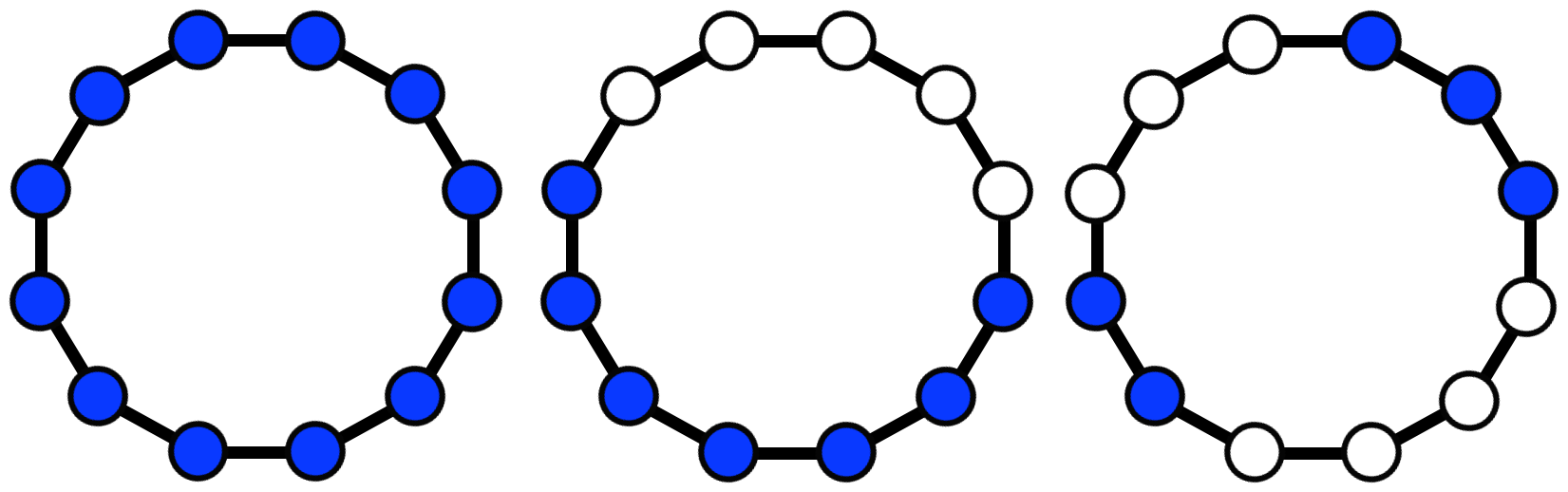
Figure 1: An illustration of ring polymer configurations with zero (left), one (center), and two (right) kink-pairs in a two-state system. The colors blue and white represent the two states of the system.

Restraining individual electronic ring polymer beads to a particular state space configuration is accomplished in the SS-PI framework by inserting appropriate projection matrices $\mathbb{P}_{n_{\alpha}}$ between the M matrices in Eq. (7), where the subscript $n_{\alpha}$ in $\mathbb{P}_{n_{\alpha}}$ refers to the state onto which we project the $\alpha^{th}$ bead:

$$\Gamma_{\left\{n_{\alpha}\right\}}=\Gamma_{n_{1},n_{2},\ldots,n_{N}}=\prod_{\alpha=1}^{N}\textbf{M}(\mathbf{R}_{\alpha})\mathbb{P}_{n_{\alpha}}.$$ (15)

We then define $\Gamma_{\text{Kinks}}$ as the sum over all possible combinations of ${\left\{n_{\alpha}\right\}}$ that correspond to kinked configurations. The specifics of generating these configurations and calculating the quantities in Eq. (14) as well as the dynamic recrossing factor are described in the implementation details section.

3.2 The Population Coordinate

Defining the TS for ET in terms of the solvent position with a weak constraint on allowed electronic state configurations is typically insufficient to describe ET models with high asymmetry (near activationless through inverted regimes of Marcus theory). To overcome this challenge, we define a TS that enforces equal populations in the electronic states at solvent configurations where the reactant and product electronic state energies are equal. The corresponding MF-RPMD dynamic recrossing factor in Eq. (12) is then computed for a normalized population-based reaction coordinate,

$$\xi\equiv\Delta\mathbb{P}=\frac{\text{Tr}[\Gamma\mathbb{P}_{2}]-\text{Tr}[\Gamma\mathbb{P}_{1}]}{\text{Tr}[\Gamma\mathbb{P}_{2}]+\text{Tr}[\Gamma\mathbb{P}_{1}]},$$ (16)

that distinguishes between reactant, TS, and product configurations in all regimes of ET:

$$\Delta\mathbb{P}=\left\{\begin{array}[]{cl}-1&\text{reactant minimum}\\ 0&\text{transition state}\\ 1&\text{product minimum}.\\ \end{array}\right.$$ (17)

For the population coordinate, the probability of reaching the TS from the reactant state in Eq.(13) is defined as

$$\text{P}\left(\mathbf{R}^{\ddagger},n^{\ddagger}\right)=\frac{\int\left\{d\mathbf{R}_{\alpha}\right\}e^{-\frac{\beta}{N}V_{N}\left(\{\mathbf{R}_{\alpha}\}\right)}\text{Tr}\left[\Gamma_{\Delta\mathbb{P}=0}\right]\delta\left(\overline{\mathbf{R}}-\mathbf{R}^{\ddagger}\right)}{\int\left\{d\mathbf{R}_{\alpha}\right\}e^{-\frac{\beta}{N}V_{N}\left(\{\mathbf{R}_{\alpha}\}\right)}\text{Tr}\left[\Gamma_{\Delta\mathbb{P}=-1}\right]},$$ (18)

where $\Gamma_{\Delta\mathbb{P}=0}$ includes only kinked configurations with an equal number of ring polymer beads in either state, $\Gamma_{\Delta\mathbb{P}=-1}$ includes only configurations where all the ring polymer beads are in the reactant state, and, in the numerator, the nuclear COM is restrained to the position at which the two electronic states are degenerate.

4 Implementation Details

4.1 Solvent Reaction Coordinate

In practice, it is easiest to evaluate the probability of forming configurations corresponding to the TS in Eq. (14) by splitting it into two terms:

$$\text{P}\left(\mathbf{R}^{\ddagger},n^{\ddagger}\right)=\text{P}\left(\mathbf{R}^{\ddagger}\right)\times\text{P}\left(n^{\ddagger}|\mathbf{R}^{\ddagger}\right),$$ (19)

where

$$\text{P}\left(\mathbf{R}^{\ddagger}\right)=\frac{\int\left\{d\mathbf{R}_{\alpha}\right\}e^{-\frac{\beta}{N}V_{N}\left(\{\mathbf{R}_{\alpha}\}\right)}\text{Tr}\left[\Gamma\mathbb{P}_{1}\right]\delta\left(\overline{\mathbf{R}}-\mathbf{R}^{\ddagger}\right)}{\int_{-\infty}^{\mathbf{R}^{\ddagger}}d\mathbf{R}^{\prime}\int\left\{d\mathbf{R}_{\alpha}\right\}e^{-\frac{\beta}{N}V_{N}\left(\{\mathbf{R}_{\alpha}\}\right)}\text{Tr}\left[\Gamma\mathbb{P}_{1}\right]\delta\left(\overline{\mathbf{R}}-\mathbf{R}^{\prime}\right)}$$ (20)

represents the probability of the system reaching the nuclear TS, $\overline{\mathbf{R}}=\mathbf{R}^{\ddagger}$, from reactants and

$$\text{P}\left(n^{\ddagger}|\mathbf{R}^{\ddagger}\right)=\frac{\int\left\{d\mathbf{R}_{\alpha}\right\}e^{-\frac{\beta}{N}V_{N}\left(\{\mathbf{R}_{\alpha}\}\right)}\text{Tr}\left[\Gamma_{\text{Kinks}}\right]\delta\left(\overline{\mathbf{R}}-\mathbf{R}^{\ddagger}\right)}{\int\left\{d\mathbf{R}_{\alpha}\right\}e^{-\frac{\beta}{N}V_{N}\left(\{\mathbf{R}_{\alpha}\}\right)}\text{Tr}\left[\Gamma\mathbb{P}_{1}\right]\delta\left(\overline{\mathbf{R}}-\mathbf{R}^{\ddagger}\right)}$$ (21)

represents the conditional probability of the system forming the electronic TS (kink-pair configurations) given that the solvent COM is at $\mathbf{R}^{\ddagger}$.

We evaluate Eq. (20) by generating a free energy profile along $\overline{\mathbf{R}}$ using umbrella sampling⁴⁰ and the weighted histogram analysis method (WHAM),⁴¹ where a harmonic restraint on $\overline{\mathbf{R}}$ is used to center simulation windows at different values $\mathbf{R}_{i}$ throughout the reactant and TS regions. In each window, nuclear configurations are generated by MC importance sampling using the weighting function

$$W_{1}=e^{-\frac{\beta}{N}V_{N}-0.5k_{c}\left(\overline{\mathbf{R}}-\mathbf{R}_{i}\right)^{2}}\text{Tr}\left[\Gamma\mathbb{P}_{1}\right].$$ (22)

In a separate simulation, Eq. (21) is evaluated by importance sampling using the weighting function

$$W_{2}=e^{-\frac{\beta}{N}V_{N}},$$ (23)

and the delta function $\delta\left(\overline{\mathbf{R}}-\mathbf{R}^{\ddagger}\right)$ is enforced by shifting the nuclear ring polymer COM to $\mathbf{R}^{\ddagger}$ for each MC step. The terms $\text{Tr}\left[\Gamma_{\text{Kinks}}\right]$ and $\text{Tr}\left[\Gamma\mathbb{P}_{1}\right]$ are evaluated at each step, and the ratio of their final averages yields $\text{P}\left(n^{\ddagger}|\mathbf{R}^{\ddagger}\right)$.

In order to calculate $\text{Tr}\left[\Gamma_{\text{Kinks}}\right]$, we must account for all combinations of the set $\left\{n_{\alpha}\right\}$ in Eq. (15) that correspond to kinked configurations. Consider a two-state system ($K=2$) for simplicity. A particular electronic configuration $\left\{n_{\alpha}\right\}~{}\equiv~{}\left\{j,w,m\right\}$ is characterized by the number of beads in state 1 which we denote as $j$, the number of kink-pairs present which we denote as $w$, and $m$ which represents the particular electronic configuration in the subset of configurations that have the same values of $j$ and $w$. Combinations for which there exist at least one kink-pair correspond to values of $j$ equal to $1$ through $N-1$, and the number of possible kink-pairs ranges from 1 to $w_{\text{tot}}$, where $w_{\text{tot}}=j$ for $j\leq N/2$ and $w_{\text{tot}}=N-j$ for $j>N/2$; values for $m$ range from 1 to $m_{\text{tot}}$, where $m_{\text{tot}}$ depends on the particular values of $j$ and $w$. For a given nuclear configuration the exact thermal weight of kink-pair configurations is

$$\text{Tr}\left[\Gamma_{\text{Kinks}}\right]=\text{Tr}\left[\sum_{j=1}^{N-1}\sum_{w=1}^{w_{\text{tot}}\left(j\right)}\sum_{m=1}^{m_{\text{tot}}\left(j,w\right)}\Gamma_{\left\{j,w,m\right\}}\right].$$ (24)

For a large number of ring polymer beads, we acheive an efficient implementation by evaluating Eq. (24) once at the beginning of the simulation to determine $m_{\text{tot}}\left(j,w\right)$. We then choose a “representative configuration” $\left\{n_{\alpha}\right\}~{}\equiv~{}\left\{j,w\right\}^{\prime}$ for every combination of $j$ and $w$. This allows us to evaluate $\text{Tr}\left[\Gamma_{\text{Kinks}}\right]$ at each MC step as a sum over representative combinations weighted by $m_{\text{tot}}\left(j,w\right)$,

$$\text{Tr}\left[\Gamma_{\text{Kinks}}\right]=\text{Tr}\left[\sum_{j=1}^{N-1}\sum_{w=1}^{w_{\text{tot}}\left(j\right)}m_{\text{tot}}\left(j,w\right)\Gamma_{\left\{j,w\right\}^{\prime}}\right],$$ (25)

which, on average, yields the same result as Eq. (24). In the weak coupling regime, sampling can be limited to configurations with $w=1$ that dominate the sum; however, in the present work we do not find it necessary to impose this limit on the number of kink-pairs. Finally, in order to evaluate $\text{Tr}\left[\Gamma\mathbb{P}_{1}\right]$ in Eq. (21) for a given nuclear configuration, we simply add to $\text{Tr}\left[\Gamma_{\text{Kinks}}\right]$ a term that corresponds to all the RP beads being in electronic state 1 ($j=N$ and $w=0$).

The average forward velocity term that appears in the numerator of the TST estimate and the denominator of the dynamic recrossing factor can be analytically obtained by evaluating a Gaussian integral in the solvent momentum:

$$\left\langle\dot{\overline{\mathbf{R}}}_{0}\;h\left(\dot{\overline{\mathbf{R}}}_{0}\right)\right\rangle_{c}=\left(\frac{1}{2\pi\beta M}\right)^{d/2}.$$ (26)

Initial configurations for MF-RPMD trajectories are generated by importance sampling using the weighting function

$$W_{3}=e^{-\frac{\beta}{N}V_{N}}\text{Tr}\left[\Gamma_{\text{Kinks}}\right],$$ (27)

and the delta function $\delta\left(\overline{\mathbf{R}}-\mathbf{R}^{\ddagger}\right)$ is enforced by shifting the nuclear COM to $\mathbf{R}^{\ddagger}$ after each MC step. Here, the term $\text{Tr}\left[\Gamma_{\text{Kinks}}\right]$ is evaluated using Eq. (25). MF-RPMD trajectories are evolved in time using the classical ring polymer Hamiltonian in Eq. (11); averaging the expression $\left(\dot{\overline{\mathbf{R}}}_{0}\;h\left(\overline{\mathbf{R}}_{t}-\mathbf{R}^{\ddagger}\right)\right)$ over all trajectories and dividing by Eq. (26) yields a value for $\kappa_{\text{MF-RPMD}}$.

4.2 Population Reaction Coordinate

As with the solvent reaction coordinate, we evaluate the probability of forming configurations corresponding to the population coordinate TS in Eq. (18) by splitting it into two terms, where

$$\text{P}\left(\mathbf{R}^{\ddagger}\right)=\frac{\int\left\{d\mathbf{R}_{\alpha}\right\}e^{-\frac{\beta}{N}V_{N}\left(\{\mathbf{R}_{\alpha}\}\right)}\text{Tr}\left[\Gamma_{\Delta\mathbb{P}=-1}\right]\delta\left(\overline{\mathbf{R}}-\mathbf{R}^{\ddagger}\right)}{\int\left\{d\mathbf{R}_{\alpha}\right\}e^{-\frac{\beta}{N}V_{N}\left(\{\mathbf{R}_{\alpha}\}\right)}\text{Tr}\left[\Gamma_{\Delta\mathbb{P}=-1}\right],}$$ (28)

and

$$\text{P}\left(n^{\ddagger}|\mathbf{R}^{\ddagger}\right)=\frac{\int\left\{d\mathbf{R}_{\alpha}\right\}e^{-\frac{\beta}{N}V_{N}\left(\{\mathbf{R}_{\alpha}\}\right)}\text{Tr}\left[\Gamma_{\Delta\mathbb{P}=0}\right]\delta\left(\overline{\mathbf{R}}-\mathbf{R}^{\ddagger}\right)}{\int\left\{d\mathbf{R}_{\alpha}\right\}e^{-\frac{\beta}{N}V_{N}\left(\{\mathbf{R}_{\alpha}\}\right)}\text{Tr}\left[\Gamma_{\Delta\mathbb{P}=-1}\right]\delta\left(\overline{\mathbf{R}}-\mathbf{R}^{\ddagger}\right)}.$$ (29)

Eq. (28) is evaluated with the same techniques used for Eq. (20), but here we employ the weighting function

$$W_{4}=e^{-\frac{\beta}{N}V_{N}-0.5k_{c}\left(\overline{\mathbf{R}}-\mathbf{R}_{i}\right)^{2}}\text{Tr}\left[\Gamma_{\Delta\mathbb{P}=-1}\right],$$ (30)

where

$$\text{Tr}\left[\Gamma_{\Delta\mathbb{P}=-1}\right]=\text{Tr}\left[\Gamma_{\left\{N,0\right\}^{\prime}}\right].$$ (31)

We evaluate Eq. (29) using an approach similar to Eq. (21), but in this case we only include kinked configurations with equal numbers of beads in each state:

$$\text{Tr}\left[\Gamma_{\Delta\mathbb{P}=0}\right]=\text{Tr}\left[\sum_{w=1}^{N/2}m_{\text{tot}}\left(N/2,w\right)\Gamma_{\left\{N/2,w\right\}^{\prime}}\right].$$ (32)

Initial configurations for the MF-RPMD simulation are generated by importance sampling using the weighting function

$$W_{5}=e^{-\frac{\beta}{N}V_{N}}\text{Tr}\left[\Gamma_{\Delta\mathbb{P}=0}\right],$$ (33)

and again we implement $\delta\left(\overline{\mathbf{R}}-\mathbf{R}^{\ddagger}\right)$ by shifting the nuclear COM to $\mathbf{R}^{\ddagger}$. Trajectories initially constrained to this TS distribution are evolved using the Hamiltonian in Eq. (11), and the average initial velocity of the population coordinate is determined by computing the rate of change of $\Delta\mathbb{P}$ for each trajectory using a finite difference approximation at very short times and averaging over the ensemble. The average forward velocity computed using this technique is then multiplied by $\text{P}\left(\mathbf{R}^{\ddagger},n^{\ddagger}\right)$ to obtain the TST rate estimate.

4.3 Rate Theories for Adiabatic and Nonadiabatic Electron Transfer

The Marcus theory (MT) rate for a nonadiabatic ET reaction with a classical solvent is ¹

$$k_{\text{MT}}=\frac{2\pi}{\hbar}{|\Delta|}^{2}\sqrt{\frac{\beta}{4\pi\lambda}}e^{-\beta\left(\lambda-\varepsilon\right)^{2}/4\lambda},$$ (34)

where $\lambda$ is the solvent reorganization energy, $\varepsilon$ is the asymmetry between the reactant and product state energies at their respective minima, and $\Delta$ is the coupling between the reactant and product diabatic electronic states.

The nonadiabatic ET rate with a quantized solvent can be calculated using Fermi’s golden rule (FGR). For systems in which the reactant and product diabatic potential energy surfaces are displaced harmonic oscillators with frequency $\omega_{s}$, FGR rates take the simple analytical form^{42, 43}

$$k_{\text{FGR}}=\frac{2\pi}{\hbar\omega_{s}}{|\Delta|}^{2}e^{vz-S\;\text{coth}\left(z\right)}I_{v}\left(S\;\text{csch}\left(z\right)\right),$$ (35)

where $z=\beta\omega_{s}/2$, $v=\varepsilon/\omega_{s}$, $S=M_{s}\omega_{s}V_{d}^{2}/2\hbar$, $M_{S}$ is the solvent mass, $I_{v}$ is a modified Bessel function of the first kind, and $V_{d}$ is the horizontal displacement of the diabatic potential energy functions.

Reaction rates for ET in the adiabatic limit with a quantum solvent can be estimated using Kramers theory (KT), ⁴⁴

$$k_{\text{KT}}=\left(\sqrt{1+\left(\frac{\gamma}{2\omega_{b}}\right)^{2}}-\frac{\gamma}{2\omega_{b}}\right)\frac{\omega_{s}}{2\pi}e^{-\beta G^{\ddagger}_{\text{cl}}},$$ (36)

where $\omega_{b}$ is the frequency that confines the barrier top, $G^{\ddagger}_{\text{cl}}$ is the solvent FE barrier when the solvent is treated classically, $\gamma~{}=~{}\eta/M_{S},$⁴⁵ and $\eta$ is the strength of coupling to a dissipative bath.

5 Model Systems

Table 1:  Parameters for ET models. Unless otherwise specified, values are reported in atomic units.

Parameter	Value Range
$A$	$4.772\times 10^{-3}$
$B$	$2.288\times 10^{-2}$
$\varepsilon$	0 - 0.2366
$\Delta$	$6.69\times 10^{-7}$ - $1.20\times 10^{-2}$
$M_{S}$	1836.0
$M_{B}$	1836.0
$f$	12
$\omega_{c}$	$2.28\times 10^{-3}$
$\eta/M\omega_{c}$	1.0
$T$	300 K

Numerical results are presented for condensed-phase ET systems with potential energy functions of the form^{46, 28}

$$V\left(\hat{\mathbf{R}}\right)=V_{S}\left(\hat{\mathbf{R}}\right)+\mathbb{1}V_{B}\left(\hat{\mathbf{R}}\right),$$ (37)

where $\mathbb{1}$ is the identity matrix and $\mathbf{R}=\left\{s,\mathbf{Q}\right\}$ represents the full set of nuclear coordinates, including both a solvent polarization coordinate, $s$, and bath coordinates, $\mathbf{Q}$. The diabatic potential energy matrix for each system, constructed along the solvent coordinate, has the form

$$V_{S}\left(\hat{\mathbf{R}}\right)=\begin{bmatrix}A\hat{s}^{2}+B\hat{s}+\varepsilon&\Delta\\ \Delta&A\hat{s}^{2}-B\hat{s}\end{bmatrix},$$ (38)

and the solvent coordinate, with associated mass $M_{S}$, is linearly coupled to a set of $f$ harmonic oscillators, with mass $M_{B}$, through the potential

$$V_{B}\left(\hat{\mathbf{R}}\right)=\sum_{j=1}^{f}\left[\frac{1}{2}M_{B}\omega^{2}_{j}\left(\hat{Q}_{j}-\frac{c_{j}\hat{s}}{M_{B}\omega^{2}_{j}}\right)^{2}\right].$$ (39)

The spectral density of the bath is Ohmic,

$$J\left(\omega\right)=\eta\omega e^{-\omega/\omega_{c}},$$ (40)

with cutoff frequency $\omega_{c}$ and dimensionless parameter $\eta$ that determines the friction strength of the bath. Following the scheme developed in Ref. 47, we discretize the spectral density into $f$ oscillators with frequencies

$$\omega_{j}=-\omega_{c}\;\text{ln}\left(\frac{j-1/2}{f}\right)$$ (41)

and coupling strengths

$$c_{j}=\omega_{j}\left(\frac{2\eta M_{B}\omega_{c}}{f\pi}\right)^{1/2},$$ (42)

where $j=1...f$. We test a range of driving force values, $\varepsilon$, as well as a range of electronic coupling strengths, $\Delta$, from the nonadiabatic to adiabatic limit. In all cases considered, we quantize all degrees of freedom with $N=32$ ring polymer beads. All other parameters are reported in Table 1.

6 Results and Discussion

We calculate nonadiabatic reaction rates for the model ET systems described in Section 5 over a wide range of driving forces, electronic coupling strengths, and with different reaction coordinates.

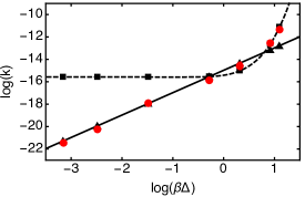
Figure 2: ET rate constants computed using the solvent reaction coordinate for a range of electronic coupling constants, $\Delta$, for the symmetric model, $\varepsilon=0$. MF-RPMD values are shown in red dots, FGR rate constants are shown in black triangles and a solid black line, and Kramers theory rate constants are shown in black squares and a black dashed line. Both axes are in atomic units.

First, we present our results for ET reaction rates using the solvent reaction coordinate for the symmetric case, Model I ($\varepsilon=0$), with different electronic coupling values. For all calculations that employ the solvent reaction coordinate, TST results are obtained using a force constant $k_{c}=200$ a.u. in umbrella sampling, and MF-RPMD results are obtained by averaging over $24,000$ trajectories evolved using a time step $dt=0.1$ a.u. In Fig. 2, we compare our results against the Kramers theory rates for adiabatic ET and FGR for nonadiabatic ET, and we show that our calculated rates exhibit quantitative agreement with the applicable theory across six orders of magnitude in the electronic coupling. Numerical values for the rate constants are reported in Table 2, along with the TST rate. We see that, despite the limitations of MF-RPMD, the accuracy of the TST rate in this regime is sufficient for good numerical agreement.

Table 2:  ET rates for a range of electronic coupling strengths, $\Delta$, for the symmetric model, $\varepsilon=0$, computed using the solvent reaction coordinate. From left to right, the four rightmost columns report the TST estimate to the rate constant, the full MF-RPMD rate constant, Fermi’s golden rule values, and Kramers theory rate constants, respectively. The numbers in parentheses represent the statistical uncertainty in the last digit reported, and all values are reported in atomic units.

$\Delta$	$\text{log}\left(k_{\text{TST}}\right)$	$\text{log}\left(k_{\text{MF-RPMD}}\right)$	$\text{log}\left(k_{\text{FGR}}\right)$	$\text{log}\left(k_{\text{KT}}\right)$
$6.69\times 10^{-7}$	-21.47	-21.47(8)	-21.28	-15.57
$3.16\times 10^{-6}$	-20.22	-20.2(2)	-19.93	-15.58
$3.16\times 10^{-5}$	-17.95	-17.9(2)	-17.93	-15.58
$5.01\times 10^{-4}$	-15.84	-15.8(1)	-15.53	-15.54
$2.00\times 10^{-3}$	-14.55	-14.6(3)	-14.33	-15.02
$7.94\times 10^{-3}$	-12.51	-12.55(4)	-13.13	-12.60
$1.20\times 10^{-2}$	-11.30	-11.3(2)	-12.77	-11.11

Next, we present the rate of ET calculated using the solvent coordinate for weak-coupling Models I-VI that explore a range of driving forces in the normal regime. Fig. 3 compares our MF-RPMD rates to FGR rates. The exact values of these rate constants are also reported in Table 3, along with the state space TST estimates. We also show the dynamic recrossing factor as a function of time in Fig. 4.

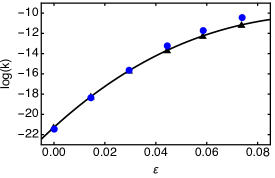
Figure 3: ET rate constants computed using the solvent reaction coordinate for a range of driving force values, $\varepsilon$, with constant coupling $\Delta=6.69\times 10^{-7}$. MF-RPMD results are shown in blue dots, and FGR rate constants are shown in black triangles and a solid black line. Both axes are in atomic units.

We find that our MF-RPMD implementation proves quantitatively accurate for ET in the normal regime. The high values of $\kappa$, particularly for the symmetric and near-symmetric models of ET, demonstrate the accuracy of our TST rate for these models. As the models become more asymmetric, $\kappa_{\text{MF-RPMD}}$ decreases, and eventually, as seen in Model VI (blue curve), at longer times we no longer observe plateau behavior (we use the value of $\kappa_{\text{MF-RPMD}}$ at $t=8000$ a.u. to obtain the reported rate constant for this model). MF-RPMD with the solvent reaction coordinate becomes inapplicable beyond Model VI–this is expected since the solvent coordinate is no longer able to distinguish between reactant and product states.

Table 3:  ET rates computed using the solvent reaction coordinate for a range of driving forces, $\varepsilon$, with constant coupling $\Delta=6.69\times 10^{-7}$. From left to right, the three rightmost columns report the TST estimate to the rate constant, the full MF-RPMD rate constant, and the Fermi’s golden rule values, respectively. The numbers in parentheses represent the statistical uncertainty in the last digit reported, and all values are reported in atomic units.

Model	$\varepsilon$	$\text{log}\left(k_{\text{TST}}\right)$	$\text{log}\left(k_{\text{MF-RPMD}}\right)$	$\text{log}\left(k_{\text{FGR}}\right)$
I	0.0000	-21.47	-21.47(8)	-21.28
II	0.0146	-18.35	-18.349(6)	-18.23
III	0.0296	-15.65	-15.670(5)	-15.66
IV	0.0446	-13.18	-13.22(1)	-13.65
V	0.0586	-11.60	-11.69(1)	-12.23
VI	0.0738	-10.18	-10.47(8)	-11.15

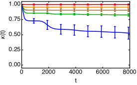
Figure 4: Plots of the dynamical recrossing term, $\kappa_{\text{MF-RPMD}}(t)$, computed using the solvent reaction coordinate as a function of time for Models I-VI (black, red, orange, brown, green, and blue, respectively) from top to bottom. Both axes are in atomic units.

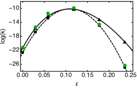
Figure 5: ET rate constants computed using the population reaction coordinate for a range of driving force values, $\varepsilon$, with constant coupling $\Delta=6.69\times 10^{-7}$. MF-RPMD results are shown in green dots, FGR rate constants are shown in black triangles and a solid black line, and MT results are shown in black squares and a black dashed line. Both axes are in atomic units.

Finally, we present our results for ET rates calculated using the population coordinate in Models I, III, and V (normal regime) and in Models VII-IX (activationless and inverted regimes). For these simulations, TST results are obtained using a force constant $k_{c}=200$ a.u. in umbrella sampling. MF-RPMD results are obtained by averaging over $30,000$ trajectories evolved using a time step $dt=0.1$ a.u., and numerical derivatives used to compute the initial $\Delta\mathbb{P}$ velocities are calculated by averaging $\left(\Delta\mathbb{P}\left(n\times dt\right)-\Delta\mathbb{P}\left(0\right)\right)/\left(n\times dt\right)$ for $n=20,30,$ and $40$. Fig. 5 shows that rates obtained using the population coordinate, like the solvent coordinate, are quantitatively accurate, agreeing with FGR rates in the normal regime. Additionally, we are able to move past Model VI to the activationless and inverted regimes (Models VII-IX), where the population coordinate remains a good reaction coordinate. The numerical values of our calculated rates, along with the TST rates, are reported in Table 4. Further, Fig. 6 shows $\kappa(t)$ for the different models; as in the previous case, $\kappa$ is approximately 1 for the symmetric model and decreases as the driving force increases.
We note that in the inverted regime our results are qualitatively reasonable and capture the predicted Marcus turnover in rates. However, we do not find quantitative agreement with FGR; instead, our results agree more closely with Marcus theory rates. We attribute this to the fact that our definition of $k_{\text{TST}}$ does not allow kinked configurations of the ring polymer to form except at solvent configurations corresponding to the point of degeneracy between the two diabats. ²⁸ We expect that either using a better formulation for the TS that can explicitly account for solvent tunneling or employing dynamics beyond mean field will improve our numerical results in the inverted regime.

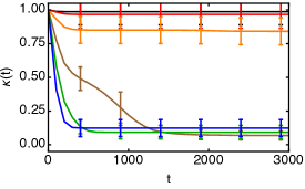
Figure 6: Plots of the dynamical recrossing term, $\kappa_{\text{MF-RPMD}}(t)$, computed using the population reaction coordinate as a function of time for Models I, III, V, and VII-IX (black, red, orange, brown, green, and blue, respectively). Both axes are in atomic units.

Table 4:   ET rates computed using the population coordinate for a range of driving forces, $\varepsilon$, with constant coupling, $\Delta=6.69\times 10^{-7}$. From left to right, the four rightmost columns report the TST estimate to the rate constant, the full MF-RPMD rate constant, Fermi’s golden rule values, and Marcus theory rate constants, respectively. The numbers in parentheses represent the statistical uncertainty in the last digit reported, and all values are reported in atomic units.

Model	$\varepsilon$	$\text{log}\left(k_{\text{TST}}\right)$	$\text{log}\left(k_{\text{MF-RPMD}}\right)$	$\text{log}\left(k_{\text{FGR}}\right)$	$\text{log}\left(k_{\text{MT}}\right)$
I	0.0000	-21.18(8)	-21.19(9)	-21.28	-22.65
III	0.0296	-15.34(4)	-15.36(6)	-15.66	-16.79
V	0.0586	-11.37(5)	-11.45(7)	-12.23	-12.83
VII	0.1186	-8.72(5)	-9.9(2)	-10.26	-10.19
VIII	0.1776	-13.50(5)	-14.5(2)	-13.20	-14.91
IX	0.2366	-25.44(7)	-26.3(2)	-19.63	-26.89

7 Concluding Remarks

We show that combining TST rates computed using a state space path integral formulation with dynamic correction factors computed using MF-RPMD yield quantitatively accurate rates for ET over a wide range of electronic coupling strengths and driving forces. This implementation is general for multi-electron, multi-state systems, and we expect the simple protocol described here to work well for large scale atomistic simulations. Moving forward, we anticipate that the state space TST implementation described here, in combination with nonadiabatic RPMD methods such as mapping variable (MV)-RPMD,²⁷ will prove extremely useful in the study of photo-induced charge transfer reactions.

References

- Marcus and Sutin 1985 R. A. Marcus and N. Sutin, Biochim. Biophys. Acta, 1985, 811, 265–322.
- Gray and Winkler 1996 H. B. Gray and J. R. Winkler, Annu. Rev. Biochem., 1996, 65, 537–561.
- Reece and Nocera 2009 S. Y. Reece and D. G. Nocera, Annu. Rev. Biochem., 2009, 78, 673–699.
- Cukier and Nocera 1998 R. I. Cukier and D. G. Nocera, Annu. Rev. Phys. Chem., 1998, 49, 337–369.
- Lewis and Nocera 2006 N. S. Lewis and D. G. Nocera, Proc. Natl. Acad. Sci. U.S.A., 2006, 103, 15729–15735.
- Feldt et al. 2013 S. M. Feldt, P. W. Lohse, F. Kessler, M. K. Nazeeruddin, M. Grätzel, G. Boschloo and A. Hagfeldt, Phys. Chem. Chem. Phys., 2013, 15, 7087–7097.
- Tully 1990 J. C. Tully, J. Chem. Phys., 1990, 93, 1061–1071.
- Kapral 2006 R. Kapral, Annu. Rev. Phys. Chem., 2006, 57, 129–157.
- Jain and Subotnik 2015 A. Jain and J. E. Subotnik, J. Chem. Phys., 2015, 143, 134107.
- Cao et al. 1995 J. Cao, C. Minichino and G. A. Voth, J. Chem. Phys., 1995, 103, 1391–1399.
- Cao and Voth 1997 J. Cao and G. A. Voth, J. Chem. Phys., 1997, 106, 1769–1779.
- Ananth et al. 2007 N. Ananth, C. Venkataraman and W. H. Miller, J. Chem. Phys., 2007, 127, 084114.
- Cotton and Miller 2013 S. J. Cotton and W. H. Miller, J. Phys. Chem. A, 2013, 117, 7190–7194.
- Lee et al. 2016 M. K. Lee, P. Huo and D. F. Coker, Annu. Rev. Phys. Chem., 2016, 67, 27.1–27.31.
- Cao and Voth 1994 J. Cao and G. A. Voth, J. Chem. Phys., 1994, 100, 5093–5105.
- Craig and Manolopoulos 2004 I. R. Craig and D. E. Manolopoulos, J. Chem. Phys., 2004, 121, 3368–3373.
- Craig and Manolopoulos 2005 I. R. Craig and D. E. Manolopoulos, J. Chem. Phys., 2005, 123, 034102.
- Hele and Althorpe 2013 T. J. H. Hele and S. C. Althorpe, J. Chem. Phys., 2013, 138, 084108.
- Althorpe and Hele 2013 S. C. Althorpe and T. J. H. Hele, J. Chem. Phys., 2013, 139, 084115.
- Hele 2016 T. J. H. Hele, Mol. Phys., 2016, 114, 1461–1471.
- Menzeleev et al. 2011 A. R. Menzeleev, N. Ananth and T. F. Miller, III, J. Chem. Phys., 2011, 135, 074106.
- Habershon et al. 2013 S. Habershon, D. E. Manolopoulos, T. E. Markland and T. F. Miller, III, Annu. Rev. Phys. Chem., 2013, 64, 387–413.
- Wilkins et al. 2015 D. M. Wilkins, D. E. Manolopoulos and L. X. Dang, J. Chem. Phys., 2015, 142, 064509.
- Kowalczyk et al. 2015 P. Kowalczyk, A. P. Terzyk, P. A. Gauden, S. Furmaniak, K. Kaneko and T. F. Miller, III, J. Phys. Chem. Lett., 2015, 6, 3367–3372.
- Kretchmer and Miller 2016 J. S. Kretchmer and T. F. Miller, III, Inorg. Chem., 2016, 55, 1022–1031.
- Richardson and Thoss 2013 J. O. Richardson and M. Thoss, J. Chem. Phys., 2013, 139, 031102.
- Ananth 2013 N. Ananth, J. Chem. Phys., 2013, 139, 124102.
- Menzeleev et al. 2014 A. R. Menzeleev, F. Bell and T. F. Miller, III, J. Chem. Phys., 2014, 140, 064103.
- Duke and Ananth 2015 J. R. Duke and N. Ananth, J. Phys. Chem. Lett., 2015, 6, 4219–4223.
- MF1 The mean field RPMD approximation is not a new idea and has been used previously to benchmark nonadiabatic PI methods by D. E. Manolopoulos, T. F. Miller III, N. Ananth, J. C. Tully, and I. R. Craig. See, for instance, “An electronically non-adi The mean field RPMD approximation is not a new idea and has been used previously to benchmark nonadiabatic PI methods by D. E. Manolopoulos, T. F. Miller III, N. Ananth, J. C. Tully, and I. R. Craig. See, for instance, “An electronically non-adiabatic generalization of ring polymer molecular dynamics,” T. J. H. Hele, MChem thesis, Exeter College, University of Oxford, 2011.
- Miller et al. 1983 W. H. Miller, S. D. Schwartz and J. W. Tromp, J. Chem. Phys., 1983, 79, 4889–4898.
- Chandler 1987 D. Chandler, Introduction to Modern Statistical Mechanics, Oxford University Press, New York, 1987.
- Frenkel and Smit 2002 D. Frenkel and B. Smit, Understanding Molecular Simulation, Academic Press, California, 2nd edn., 2002.
- Trotter 1959 H. F. Trotter, Proc. Amer. Math. Soc., 1959, 10, 545–551.
- Chandler and Wolynes 1981 D. Chandler and P. G. Wolynes, J. Chem. Phys., 1981, 74, 4078–4095.
- Kuki and Wolynes 1987 A. Kuki and P. G. Wolynes, Science, 1987, 236, 1647–1652.
- Marchi and Chandler 1991 M. Marchi and D. Chandler, J. Chem. Phys., 1991, 95, 889–894.
- Ceperley 1995 D. M. Ceperley, Rev. Mod. Phys., 1995, 67, 279–355.
- Richardson and Althorpe 2011 J. O. Richardson and S. C. Althorpe, J. Chem. Phys., 2011, 134, 054109.
- Torrie and Valleau 1977 G. M. Torrie and J. P. Valleau, J. Comput. Phys., 1977, 23, 187–199.
- Kumar et al. 1992 S. Kumar, J. M. Rosenberg, D. Bouzida, R. H. Swendsen and P. A. Kollman, J. Comput. Chem., 1992, 13, 1011–1021.
- Ulstrup and Jortner 1975 J. Ulstrup and J. Jortner, J. Chem. Phys., 1975, 63, 4358–4368.
- Ulstrup 1979 J. Ulstrup, Charge Transfer Processes in Condensed Media, Springer Verlag, Berlin, 1979.
- Henriksen and Hansen 2008 N. E. Henriksen and F. Y. Hansen, Theories of Molecular Reaction Dynamics, Oxford University Press, New York, 2008.
- Makri 1996 N. Makri, J. Chem. Phys., 1996, 106, 2286–2297.
- Topaler and Makri 1994 M. Topaler and N. Makri, J. Chem. Phys., 1994, 101, 7500–7519.
- Craig and Manolopoulos 2005 I. R. Craig and D. E. Manolopoulos, J. Chem. Phys., 2005, 122, 084106.