The Physics of Biofilms – An Introduction

Abstract

Biofilms are complex, self-organized consortia of microorganisms that produce a functional, protective matrix of biomolecules. Physically, the structure of a biofilm can be described as an entangled polymer network which grows and changes under the effect of gradients of nutrients, cell differentiation, quorum sensing, bacterial motion, and interaction with the environment. Its development is complex, and constantly adapting to environmental stimuli. Here, we review the fundamental physical processes the govern the inception, growth and development of a biofilm. Two important mechanisms guide the initial phase in a biofilm life cycle: (i) the cell motility near or at a solid interface, and (ii) the cellular adhesion. Both processes are crucial for initiating the colony and for ensuring its stability. A mature biofilm behaves as a viscoelastic fluid with a complex, history-dependent dynamics. We discuss progress and challenges in the determination of its physical properties. Experimental and theoretical methods are now available that aim at integrating the biofilm’s hierarchy of interactions, and the heterogeneity of composition and spatial structures. We also discuss important directions in which future work should be directed.

I Introduction

Biofilms are among the most ancient evidence of life on Earth: they appear as fossils of microbial mats and stromatolites from western Australia dating back to about 3.5 billion years ago noffkeAstrobiology2013 ; VanKranendonkPreRea2008 . Thus, it should come as no surprise that biofilms are the most widespread form of life flemmingNatRM2010 . They form extremely diverse and complex structures, are capable of colonizing almost every environment, and have evolved a vast arsenal of biological responses to environmental stimuli. Today we know that all three domains of life can produce biofilms: bacteria hallNatRM2004 , archaea orellARMB2013 , microalgae Leadbeater1992 and fungi fanningPLOSPATHOG2012 ; ramageCRMB2009 all produce biofilms. But the understanding that most microorganisms live in aggregates rather than in a planktonic state has only recently emerged. Antonie van Leeuwenhoek observed “animalcules” in the plaque of his own teeth under a microscope of his fabrication. His report in $1676$ marks the discovery of biofilms porterBacterRev1976 . However, only in the first half of the twentieth century with the work of Henrici henriciJBacter1933 and Zobel zobellJBacter1943 was the import of biofilms really appreciated by the scientific community, and finally the word biofilm was first used in 1981 mccoyCanJMB1981 , which marks the recognition of its function and organization.

Biofilms are structured, self-organized communities of microorganisms that synthesize a protective matrix and adhere to each other and/or to an interface otooleARMB2000 ; vertPAChem2012 . They can be populated by a single species but more often multiple species are present. The level of complexity and specialization present in biofilms brings to mind the analogy to a large, bustling city watnickJBacter2000 with different levels of organization berkScience2012 . Biofilms can grow on solid surfaces in the presence of water virtually anywhere, for example on pebbles in a river bed (the periphyton), in deep-sea hydrothermal systems reysenbachTrendsMB2001 and vents taylorAEMB1999 , or on boat hulls; biofilms can also grow at the air-water interface of limnic or marine environments wotton2005surface . Like the inhabitants of a city, the microorganisms in a biofilm can modify their surroundings. Cellular metabolism can either increase the porosity of geologic media by the dissolution of minerals, or reduce the porosity by precipitating secondary minerals or by clogging the pores with biomass. Microbial activity can change the electrochemical properties, surface roughness, elastic moduli, stiffness, as well as seismic and magnetic properties of minerals through the precipitation of bacterial magnetosomes. In general, biofilms play a role in so many geophysical processes that a new discipline is now emerging: biogeophysics atekwanaRGeophysics2009 .

Biofilms play a role also in human activities. Their growth has an enormous impact in biomedical sciences SihorkarPharmaReas2001 . Microbial ecosystems can grow on the surface of teeth and on open wounds; they can infest the respiratory mucous and the airways of patients with cystic fibrosis pneumonia. Pseudomonas aeruginosa, for example, lives normally (and harmlessly) on our skin but if it enters the blood circulation of immunocompromised individuals it can infect organs of the urinary and respiratory system, bones and joints. Medical devices such as catheters, prosthetic heart valves, cardiac pacemakers, skull implants, cerebrospinal fluid shunts and orthopedic devices can harbor pathogens pavithraBiomedMaterials2008 ; hallNatRM2004 , and due to the intimate contact of these medical tools with the human body biofilms can grow and trigger virulent infections.

Biofilms cause billions of dollars in damage to metal pipes in the oil and gas industry, and metal structures in water treatment plants. Sulfate-reducing bacteria, for example members of the Acidithiobacillus genus, transforms molecular hydrogen into hydrogen sulfide which, in turn, produces sulfuric acid that corrodes metal surfaces causing catastrophic failures haoCREST1996 ; hamiltonAnnRevMB1985 ; muyzerNatRevMB2008 .

Biofilms have, however, also found useful employment in environmental biotechnology. They are used in a well-established technique for wastewater treatment nicolellaJBiotech2000 ; duBiotechAdv2007 ; DeBeer2013 , or for in situ immobilization of heavy metals in soil dielsRevEnvSciTech2002 ; gaddGeoder2004 . Biofilms allow to process large volumes of liquids, and they naturally grow by converting organic materials. Furthermore, microorganisms (typically bacteria and fungi) can be used for microbial leaching, that is, as a way to extract metals from ores sandApplMBBiotech1995 ; suzukiBiotechAdv2001 . Copper, uranium and gold are examples of metals commercially recovered by microorganisms boseckerFEMSMBRev1997 .

Figure 1: (a) Pictorial representation of a biofilm produced by a community of microorganisms. Different cellular shapes represent different species of microorganisms coexisting in the same biofilm, while different colors represent phenotypic variations within the same species. (b) Zoomed-in view of the main components of a biofilm, underlying the complexity of its physico-chemical properties: the extracellular polymeric substance and cells. We highlight (i) the cellular membrane, (ii) proteins embedded in the membrane, (iii) pili, (iv) extracellular DNA, (v) polysaccharides, (vi) proteins, (vii) lipids. Inspired by a sketch in Ref. flemmingNatRM2010 .

Numerous experimental studies have determined that biofilms have a heterogeneous structure and composition lawrenceJBact1991 ; caldwellJApplBact1993 ; costertonJBact1994 ; gjaltemaBiotechBioeng1994 ; stoodleyBiotechBioeng1999 ; stoodleyAnnRevMB2002 ; blauertBiotechBioeng2015 which vary greatly among different species. But we also know that they share some fundamental elements. Microorganisms colonizing an interface produce a mass of biopolymers, collectively termed extracellular polymeric substance (EPS), that provides protection and structural stability to the cells. The EPS also performs numerous functions specific to the biofilm state, such as creating its three-dimensional architecture, protection against physical, chemical and biological agents, providing an external digestive system, facilitating cell-cell signaling and horizontal gene transfer madsenFEMSImmun2012 .

The EPS matrix represents up to $90\%$ of the dry mass of the biofilm (the remaining being the cells) and is composed of polysaccharides, proteins, humic acids, DNA, lipids, and remnants of lysed cells flemmingNatRM2010 . (However, there are exceptions: some strains of Staphylococcus epidermidis and Staphylococcus aureus produce smaller amounts of EPS.) Figure 1 shows a sketch of a biofilm with its primary elements. Below, we briefly describe these components and highlight their functions in the biofilm.

$\cdot$ Polysaccharides are long, linear or branched, polymeric chains that are ubiquitously found in biofilms, and represent their largest component wingenderMEthEnzym2001 ; flemmingJBact2007 . The number and diversity of these molecules is stunning. Very little can be said in general about them as the number of chemical and structural possibilities is virtually infinite christensenJBiotech1989 ; sutherland1977 . Gram-negative bacteria typically produce polyanionic polysaccharides, or in some cases neutral ones, due to the presence of uronic acids or ketal-linked pyruvates; some chemical linkages ($1,3$- or $1,4$-${\beta}$-linked hexose) provide backbone rigidity to the polymers, while other linkages produce more flexible polymers sutherlandMB2001 .

Diverse microscopy methods wingender2012 ; lawrenceAEMB2003 show that polysaccharides form a complex network of fine strands linking cells to each other and to the substratum. Polysaccharides are involved in most processes that take place in a biofilm flemmingNatRM2010 : (i) adhesion; for example, the polysaccharides Pel and Psl (named after the operons involved in pellicle formation and polysaccharide synthesis locus, respectively ryderCurrOpMB2007 ) are essential for the adhesion of Pseudomonas aeruginosa to a variety of substrata and they provide redundant mechanisms for this task colvinEnvirMB2012 ; maJBacter2006 ; cooleySoftMatt2013 . (ii) Structural stability and cohesion; the polysaccharides of algae form rigid structures because the binding (chelation) of Ca²⁺ or Sr²⁺ ions forms cross-linked polymer networks donlanEID2002 ; sutherlandMB2001 . Because bacterial polysaccharides are often acetylated, the interaction between polymers is reduced and so is the resulting network-forming ability sutherlandMB2001 ; for example, Pseudomonas fluorescens requires an acetylated form of cellulose for the effective colonization of the air-liquid interface spiersMolMB2003 , and N-acetylglucosamines are crucial for intercellular adhesion in the biofilm of Staphylococcus epidermidis gotzMolMB2002 ; mackJBacter1996 , a major cause of nosocomial infections. (iii) Hydration; polysaccharides can bind water molecules (for example, hyaluronic acid can bind the considerable amount of $1$ kg of water per $1$ g of saccharide sutherlandMB2001 ; however, most molecules will probably bind less). Because the polysaccharides form an entangled polymer network they are subject to an osmotic pressure $\Pi$ such that will swell with water until the shear modulus of the network $G\approx\Pi$ seminaraPNAS2012 ; wilkingMRS2011 ; rubinstein2003 . A hydraulic decoupling between unsaturated soil bacteria and the vadose zone has been hypothesized to protect the cells from cycles of wetting and drying events orVadose2007 . (iv) Storage of nutrients; both the polysaccharide network itself and absorbed organic matter serve as a source of carbon during periods of nutrient deprivation freemanLimnolOcean1995 . (v) Protection from toxic ions; the exopolysaccharides can adsorb toxic ions such as Cd, Zn, Pb, Cu, and Sr norbergBiotechBioeng1984 ; wingender2012 ; for example, Pseudomonas aeruginosa in a biofilm is up to $600$ times more resistant to Zn, CU and Pb than in the planktonic state teitzelApplEnvMB2003 . (vi) Antibiotic protection; Pseudomonas aeruginosa infecting cystic fibrosis patients can change to a mucoid phenotype characterized by increased production of the polysaccharide alginate, but the biofilm contains also Pel and Psl. All three components have been found to have a protective role against antibiotics hentzer2001alginate ; colvinPLOS2011 ; billingsPLOS2013 . (vii) Reservoir of enzymes; enzymes are stored, accumulated and stabilized by the polysaccharide network wingender1999 ; for example, it has been suggested lockOikos1984 that epilithic biofilms of microorganisms growing on river beds (a highly changeable environment) benefit from the accumulation of enzymes because, firstly, the products of enzymatic activity are readily available to the cells, secondly, they may additionally trigger new enzymatic activity in adjacent cells, and, thirdly, new generations do not need to spend energy on enzyme synthesis. (viii) Sink for excess carbon; when supplied with excess C, the production of polysaccharides is greatly enhanced oteroJPhyco2004

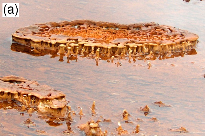
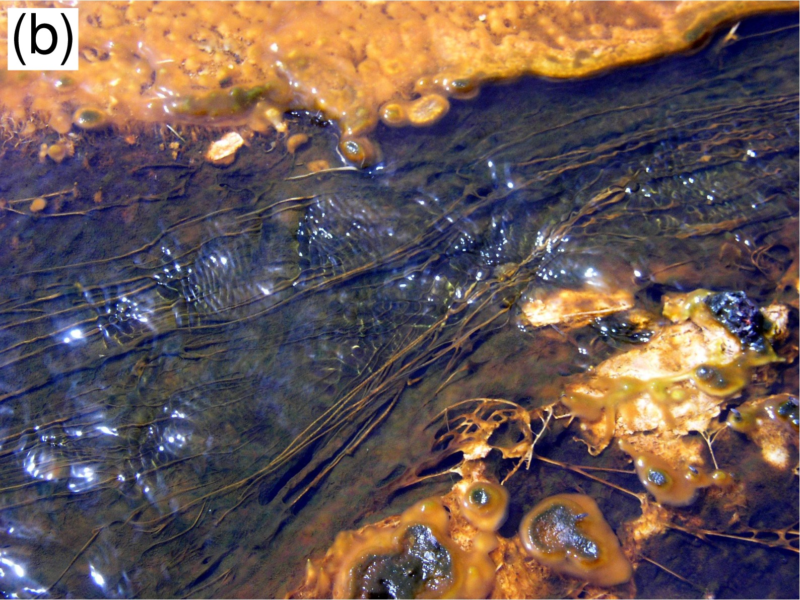
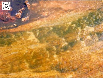
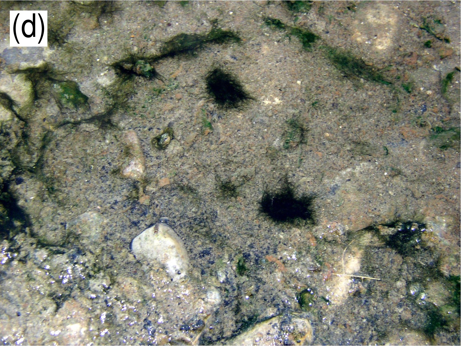
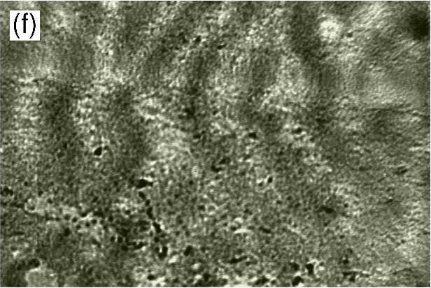
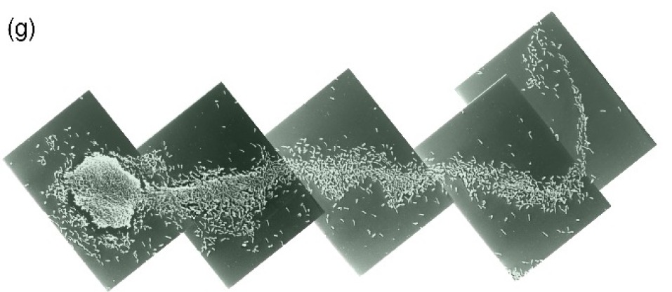
Figure 2: Examples of biofilms growing in different environments. (a-c) Biofilms growing in hydrothermal hot springs from the Biscuit Basin thermal area, Yellowstone National Park, USA; (d) Gardener River, Yellowstone National Park, USA; (e) Hyalite Creek, Bozeman, Montana, USA; (f-g) Pseudomonas aeruginosa PAN067 biofilm grown in a flow cell with a flow of $1$ m/s. Biofilms growing in stagnant waters tend to form round, mushroom-like structures, as in (a) and (d), while biofilms growing under hydrodynamic flow form ripples, as in (c) and (f), and streamers, as in (b), (e) and (g). Images courtesy of Dr. P. Stoodley. Reprinted with permission from Ref. hallNatRM2004 .

$\cdot$ Extracellular DNA has been found not to be merely debris left from lysed cells but an actively produced component of the EPS that plays a crucial role in the formation and structural integrity of the biofilms of Variovorax paradoxus and Rhodococcus erythropolis steinbergerApplEnvMB2005 . Extracellular DNA functions as an intercellular connector in Pseudomonas aeruginosa’s biofilms yangMB2007 ; also, if these biofilms are younger than $60$ hours they can be dissolved by enzymatic degradation of the extracellular DNA whitchurchScience2002 . The Gram-positive Bacillus cereus employs extracellular DNA as an adhesin vilainApplEnvMB2009 . Recently, a novel function of extracellular DNA has been recognized: antimicrobial activity. By binding and sequestering cations, extracellular DNA induces physical alterations in the bacterial outer membrane mulcahyPLOSPath2008 .

$\cdot$ Lipids or biosurfactants modify the hydrophobic character of microbial cells and therefore can modify their ease of adhesion to surfaces. For example, lipopeptides produced by Bacillus subtilis change the hydrophobicity of the cells depending on the initial level of hydrophobicity ahimouEnzMBTech2000 . These functions are also used to protect the biofilm from invading microorganisms. In the late stages of its biofilm, Pseudomonas aeruginosa produces rhamnolipids that can disrupt biofilms formed by Bordetella bronchiseptica irie2005pseudomonas or inhibit the attachment of a variety of bacteria and yeasts rodriguesJAMB2006 . Bacillus subtilis and licheniformis produce biorsurfactants that selectively prevent the adhesion of pathogenic cells RivardoApplMBBiotech2009 .

$\cdot$ Proteins are a large component of the EPS and have diverse functions. As enzymes they form an external digestive system for the microorganisms in the biofilm as they break down biopolymers to low-molecular-mass products that can be utilized by the cells flemmingNatRM2010 . Enzymes can degrade the EPS matrix romaniMBEcol2008 ; zhangChemosph2003 or protect against oxidizers elkinsApplEnvironMB1999 .

Finally, non-enzymatic proteins contribute to the structural stability of the EPS network by attaching the cellular surface to the polysaccharides. Lectins are one such class barondesScience1984 . For example, lectins contribute to thicker biofilms in different environmental conditions in Pseudomonas aeruginosa diggleEnvMB2006 ; the presence of a plant lectin can greatly influence the biofilm of a rhizobium perezIntJMB2009 .

In addition to their composition, also the temporal development of biofilms is structured. Five stages have been recognized in the life-cycle of a biofilm stoodleyAnnRevMB2002 : (i) the initial attachment of cells to a surface or substratum; (ii) production of EPS and irreversible attachment; (iii) development of the biofilm architecture; (iv) maturation of the structure and composition of the biofilm; (v) dispersal of individual cells from the biofilm that revert to the planktonic phenotype to find a new niche and that close in this way the life-cycle of the biofilm. During dispersal the EPS matrix immobilizing the cells is broken down. This last stage of the biofilm’s life-cycle allows the colonization of new interfaces and it may be necessary when the microenvironment becomes unfavorable to sessile microorganisms. Dispersal is a highly complex process karatanMBMolBiolRev2009 ; donlanEID2002 involving the production of enzymes to degrade the EPS network sauerJBact2004 , production of surfactants bolesMolMB2005 , and induction of motility jacksonJBact2002 . For more details regarding the important phase of dispersal we refer the reader to a useful review mcdougaldNatRevMB2012 .

The possibility that the vast majority of microorganisms can form biofilms points to a strong evolutionary incentive for this cooperative behavior. Biofilms growing in different environments show strikingly similar responses to similar physical stimuli. As Fig. 2 shows, fast-moving waters produce similar morphologies called “streamers” in very different environments. Quiescent waters induce instead biofilms with more rounded morphologies hallNatRM2004 . These facts point to convergent survival strategies within a biofilm. Indeed, social interactions in microorganisms have been recognized crespiTrendsEcolEvol2001 . The advantages of a biofilm mode of life consists not only of the protection from toxins, dehydration, antibiotics, starvation, but also of a synergetic consortium that enhances immensely the chances of survival by sharing resources and allowing differentiation, for example.

For all the reasons mentioned above, it is not surprising that the study of biofilms has attracted enormous interest in microbiology, pharmacology, medicine, industry, and in more recent years also in physics. In fact, the formation, growth, organization and structure of a biofilm are all processes that need to be understood from a physical point of view. In this Review we explore a selection (far from being exhaustive) of key physical processes taking place in a biofilm. The first important step is the motility. Different kinds of motilities occur in two phases of the biofilm life-cycle: stage (i), the attachment, and stage (v), the dispersal. Next, the process of adhesion is decisive for the formation and growth of a stable biofilm. Finally, the mature biofilm resulting from myriad interactions and history-dependent dynamical responses can be viewed, on a macroscopic level, as a biomaterial, that is susceptible of physical characterization.

The topic we address in this review has a multitude of aspects and spans such a broad range of disciplines (from biochemistry and genetics to hydrodynamics and rheology) that we cannot hope to give a complete depiction of the current knowledge about biofilms. However, we have made efforts to provide a rather general picture that at least points to the most eminent physical aspects. At times, this work might appear as pedagogical. This is intended. We hope in fact that experts in one discipline will find the discussions of other disciplines connected to biofilms helpful. For further study we direct to more detailed reviews, such as Ref. shapiroAnnRevMB1998 for the concept of multicellularity, and Ref. benAdvPhys2000 for the self-organization of microorganisms. One glaring aspect of biofilm that we neglect is the genetic and regulatory network of signals that controls the biofilm’s formation, maturation and dispersal. For these topics we recommend the specialized reviews otooleARMB2000 ; karatanMBMolBiolRev2009 ; kaplanJDentRes2010 ; mcdougaldNatRevMB2012 .

This work is organized as follows. In Sec. II we discuss various mechanisms of cellular motility, from the problem of swimming at low Reynolds numbers to surface motility. Section III describes the fundamental physical processes that allow cells to adhere to solid surfaces and thus initiate a biofilm. In Sec. IV we discuss the viscoelastic behavior of biofilms as materials and the main physical concepts used in the literature. In Sec. V we describe modern advances in the experimental investigation of biofilms propelled by the fields of microfluidics and nanofabrication. In Sec. VI we review the theoretical and computational models of biofilm growth and dynamics. Finally in Sec. VII we summarize our conclusions.

II Motility

Why is motility relevant to biofilms? The first, obvious answer is that the approach of microorganisms to a surface is the first step to the constitution of a biofilm. This corresponds to stage (i) in the life-cycle of a biofilm. For example, prior to attachment and initiation of a biofilm Vibrio cholerae scans a surface by swimming in its close proximity, using two strategies called roaming and orbiting, which differ in the radius of gyration of the trajectories teschlerNRMB2015 . Swimming is also relevant in the last stage of a biofilm’s life-cycle: the dispersal. Cells of Pseudomonas aeruginosa swim away from the internal regions of the biofilm into the bulk liquid to regain access to fresh nutrients sauerJBact2002 . It is often claimed that once formed biofilms are communities of sessile microorganisms. A new picture has emerged where motility, at least in some species, plays a significant role in the biofilm’s structure formation tolkerJBact2000 ; barkenEnvMB2008 , with spatial and temporal heterogeneities in phenotypic differentiation and organization tolkerJBact2000 ; vlamakisGeneDevel2008 . It must be said, however, that living organisms exhibit a stunning variety of behaviors that refuse to be easily categorized. In fact, non-swimming species, such as Staphylococcus epidermidis and Staphylococcus aureus can also form biofilms. Thus, swimming motility is by all means not a necessary condition for biofilm formation. The inevitable generalizations sometimes present in this work should be understood from a physical point of view and not biological: that the physical processes discussed below have been shown to take place in some species does not imply that all biofilm-forming microorganisms display the same characteristics, but rather that they belong to the “toolbox” of physical mechanisms available to some species and/or phenotypes, and, as our knowledge of biofilms expands, one should consider that these physical processes might be at play.

Six different kinds of motility have been identified among $40$ bacterial species belonging to $18$ different genera henrichsenBactRev1972 : swimming, swarming, gliding, twitching, sliding and darting (see Fig. 3 for a sketch of the most important motility modes). Except for swimming, all other modes are associated to the presence of a surface. Swimming at or near a surface is actuated through one or more flagella. Let us consider one of the most studied motile bacteria: Escherichia coli. It exhibits on average six flagella, $5$ to $10\,\mu$m long and $20$ nm thick, randomly distributed around its body. The flagellum is composed of a basal body (embedded in the cellular membrane), a hook and a filament, that is, a left-handed helix with a pitch of about $2.5\,\mu$m and a diameter of about $0.5\,\mu$m turnerJBact2000 . When the flagellar motor, driven by the proton motive force, rotates counterclockwise (CCW) a helical wave travels along the filament. When all flagella rotate CCW mechanical and hydrodynamical forces group the flagella in a single bundle that propels the bacterium in roughly straight trajectories with speeds up to $40\,\mu$m/s. While the bundle rotates CCW at about $100$ Hz the cell body rotates clockwise (CW) at about $25$ Hz bergCurrBiol2008 because of conservation of angular momentum. When one or more flagellar motors rotate CW those filaments undergo a polymorphic transition to a right-handed helix. The bundle of flagella divides and a random reorientational motion called “tumbling phase” results. The tumbling phase allows the cells to change swimming direction, and it is regulated by the chemotactic signal transduction network parkinsonCell1993 .

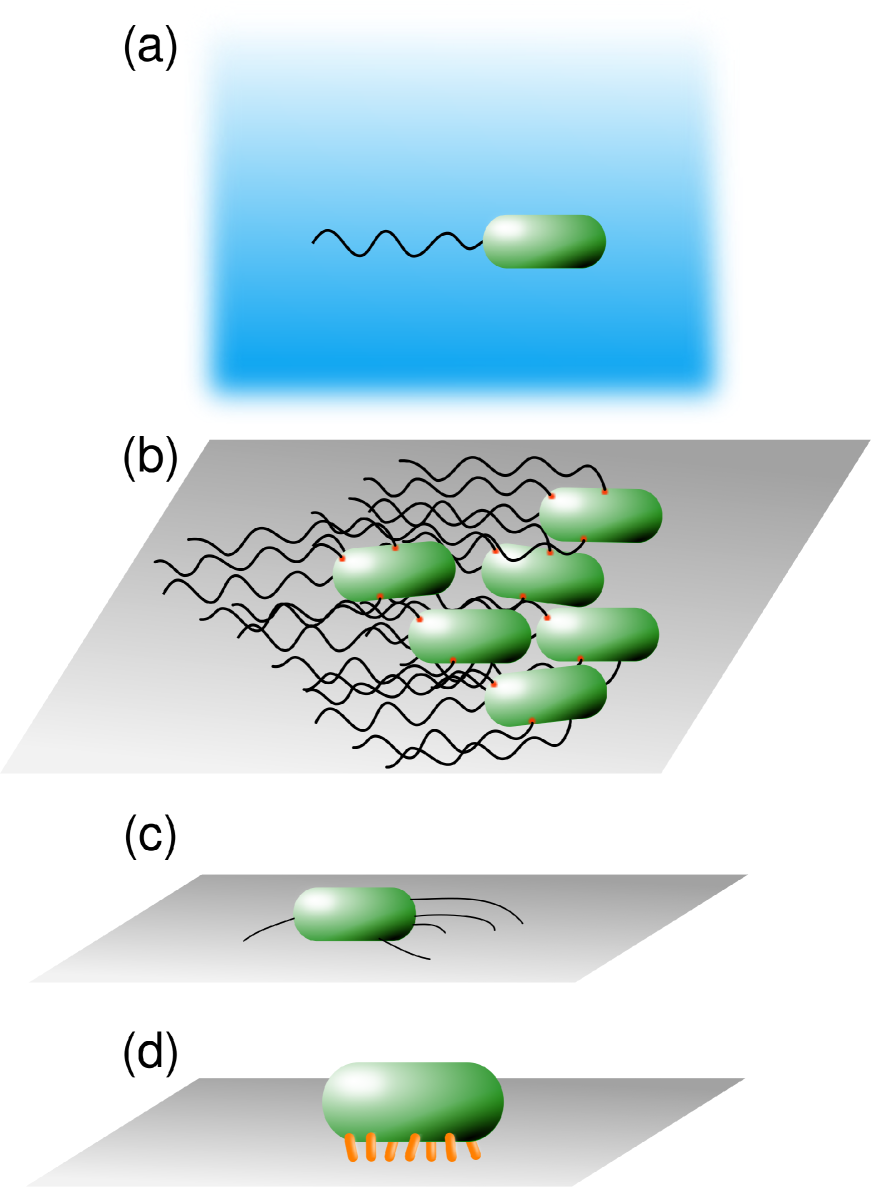
Figure 3: Pictorial representation of different motility modes of microorganisms. (a) Swimming in a bulk fluid by means of single polar flagellum; (b) bacteria in the hyperflagellated state swarming on a solid surface; (c) twitching by means of type IV pili; (d) gliding by means of focal adhesion complexes.

Escherichia coli’s flagellum has a torsional spring constant $k_{\theta}\approx 4\times 10^{-12}$ dyne cm rad^-1 blockNature1989 , but only up to twist angles of $100\degree$; for larger twist angles a second regime appears with an order of magnitude stiffer response blockNature1989 . One possible explanation for these two regimes of the flagellar compliance is that the hook exhibit a soft component, which dominates the initial phase of the twist, and the filament has a stiffer compliance, which dominates larger twist angles. This mechanism has the advantage of removing discontinuities in the motion of the motor, whose dynamics is intrinsically stochastic because it is powered by the passage of protons, which is a Poisson process. Hence the waiting times between events is an exponentially distributed random quantity bergAnnRevBiochem2003 .

A microorganism cannot swim like a fish for a simple physical reason: the viscous drag dominates the motion laugaRepProgPhys2009 . Motile cells must instead adopt a different strategy that uses drag forces to their advantage. In the next section we discuss the hydrodynamic fundamentals of bodies swimming in a viscous fluid. This is a fascinatingly vast topic. For more details we recommend specialized works on the general problem of swimming  laugaRepProgPhys2009 ; kochARFM2011 ; happel2012 , or swarming copelandSoftMatt2009 .

II.1 Swimming at low Reynolds numbers

We now discuss the general physical mechanism that produces propulsion in microorganisms that posses flagella or cilia. On general grounds, the motion of a body immersed in an aqueous environment, that is, a Newtonian fluid, is described by the Navier–Stokes equations

$$\rho\left(\frac{\partial\vec{v}}{\partial t}+\vec{v}\cdot\nabla\vec{v}\right)=-\nabla p+\eta\nabla^{2}\vec{v}\,,$$ (1)

$$\nabla\cdot\vec{v}=0\,,$$ (2)

where $\rho$ is the fluid density, $\vec{v}$ the flow velocity, $p$ the pressure, $\eta$ the viscosity, $t$ is time, and “$\cdot$” is the symbol of scalar product. Physically, Eq. (1) represents conservation of linear momentum in the fluid, and Eq. (2) the condition of incompressibiliy of the fluid. The presence of a body immersed in the fluid is incorporated by the boundary conditions necessary to solve Eq. (1)-(2). The no-slip boundary condition (valid for viscous fluids) states that at the boundary $S$ of the body $\vec{v}_{\mathrm{fluid}}(S)=\vec{v}_{\mathrm{solid}}(S)$. Solving the Navier–Stokes equations means obtaining expressions for $\vec{v}$ and $p$ that satisfy Eq. (1)-(2) and the boundary conditions.

From this knowledge, the stress tensor $\bm{\sigma}$ can be calculated. For a fluid the stress tensor can be decomposed as $\bm{\sigma}=-p\bm{\mathrm{I}}+\bm{\tau}$, where $\bm{\mathrm{I}}$ is the unit tensor, that is, into a term corresponding to the pressure stresses, which are isotropic, and a second term called deviatoric stress tensor $\bm{\tau}$ that includes viscous (shear) or other stresses. For a Newtonian fluid the deviatoric stress depends linearly on the instantaneous values of the velocity gradient, so that one can write

$$\bm{\sigma}=-p\bm{\mathrm{I}}+\eta\left[\nabla\vec{v}+\nabla\vec{v}^{\,\mathrm{T}}\right]\,,$$ (3)

where the superscript ‘T’ indicates matrix transposition. Once $\bm{\sigma}$ is found, the total hydrodynamic force $\vec{F}$ and torque $\vec{\tau}$ acting on the swimming body can be derived from integrals over its surface

$$\vec{F}=\int_{S}\,\bm{\sigma}\cdot\vec{n}\,\mathrm{d}S\,,\quad\quad\vec{\tau}=\int_{S}\,\vec{r}\times\bm{\sigma}\cdot\vec{n}\,\mathrm{d}S$$ (4)

where $\vec{n}$ is a unit vector normal to the surface.

Equation (1) represent a balance of inertial forces (the left-hand side) and viscous forces (the term $\eta\nabla^{2}\vec{v}$), thus it is natural to find a way to quantify the relative importance of inertial to viscous forces. The Reynolds number $\mathcal{R}=\rho\,UL/\eta$, where $U$ is the typical velocity and $L$ the characteristic length scale of the swimmer, gives a dimensionless measure of this balance. For a typical microorganism such as Escherichia coli ($L\approx 2\,\mu$m) swimming in water ($\rho\approx 10^{3}$ kg/m³, $\eta\approx 10^{-3}$ Pa$\cdot$s) with a typical speed $U\approx 20\,\mu$m/s the Reynolds number $\mathcal{R}\approx 10^{-5}$. It is then clear that to study the swimming of microorganisms we can neglect the inertial term in Eq. (1). In this limit the flow obeys the Stokes equations

$$\nabla p=\eta\nabla^{2}\vec{v}\,,\quad\quad\nabla\cdot\vec{v}=0\,.$$ (5)

Because the Stokes equation is linear and because of Eq. (4) the forces acting on the swimming body are directly proportional to the flow velocities guyonBookhydrodyn . Because the displacement of a solid body can be decomposed at any instant of time as the superposition of a translation with velocity $\vec{V}(t)$ and a rotation with angular velocity $\vec{\Omega}(t)$ (this is the Mozzi–Chasles theorem), the instantaneous local velocity of a point can be written as

$$\vec{v}=\vec{V}+\vec{\Omega}\times\vec{r}\,.$$ (6)

The hydrodynamic force and torque then obey the equations

$$F_{i}=-\eta(A_{ij}V_{j}+B_{ij}\Omega_{j})\,,$$ (7)

$$\tau_{i}=-\eta(C_{ij}V_{j}+D_{ij}\Omega_{j})\,.$$ (8)

Physically, the matrices $A_{ij}$ and $D_{ij}$ represent the coupling of forces to translations, and of torques to rotations, respectively, while the matrices $B_{ij}$ and $C_{ij}$ represent cross-term couplings between forces and rotations, and between torques and rotations. Dimensionally, the coefficients of $A_{ij}$ have dimensions of length, $B_{ij}$ and $C_{ij}$ of an area, and $D_{ij}$ of a volume. Because of very general arguments guyonBookhydrodyn , which do not depend on the shape of the moving body, these matrices obey the relations

$$A_{ij} =A_{ji}\,\,, D_{ij} =D_{ji}\,\,, B_{ij}=C_{ji}\,\,,$$ (9)

thus, the matrices $B_{ij}$ and $C_{ij}$ are always the transpose of each other. This means that there is a reciprocity principle for the motion in viscous fluids: the force on a rotating body and the torque on a translating body have the same coupling coefficients.

A moving body with the symmetry of a cube or a sphere will have $B_{ij}=0$, and $A_{ij}=\lambda\delta_{ij}$, where $\delta_{ij}$ is the unit matrix. Physically, the drag force on the body will be collinear with the direction of motion, $\vec{V}$. But, for a general shape, the matrix $A_{ij}$ will not be proportional to the unit matrix; thus, there will be drag anisotropy: $\vec{F}\cdot\vec{V}<0$, that is, force and velocity are not collinear and the sign indicates the energy loss due to viscous dissipation guyonBookhydrodyn . For example, for a prolate ellipsoid of revolution with one axis much larger than the other, $\ell_{1}\gg\ell_{2}$, the matrix $\mathbf{A}=A_{\|}\hat{e}\otimes\hat{e}+A_{\perp}(\mathbf{I}-\hat{e}\otimes\hat{e})$, with $A_{\perp}\approx 2A_{\|}$, where $\hat{e}$ is the unit vector (versor) in the direction of the long axis of the ellipsoid, $\otimes$ the tensor product. Physically, this means that the drag force normal to the long axis is twice as large than along it.

Drag anisotropy is the key physical effect that makes locomotion possible at low Reynolds numbers. Consider for example a thin filament, like a bacterial flagellum, deformed by a periodic wave-form. For simplicity we assume that the cell moves along the $x$ axis, and each point on the flagellum moves only in the normal direction to the $x$ axis. A short segment of the filament can be approximated by a straight, thin rod that experiences a viscous drag $\vec{f}=\vec{f}_{\|}+\vec{f}_{\perp}=-\xi_{\|}\vec{v}_{\|}-\xi_{\perp}\vec{v}_{\perp}$, where $\xi_{\perp}\approx 2\xi_{\|}$, and $\vec{v}_{\|}$ and $\vec{v}_{\perp}$ are the components of the velocity parallel and perpendicular to the segment tangent, that is, $v_{\|}=v\cos\theta$, $v_{\perp}=v\sin\theta$. The drag forces have components along the $x$ axis: $f_{\|x}=f_{\|}\sin\theta$, $f_{\perp x}=f_{\perp}\cos\theta$. The total force along the x axis, or the propulsion force then results $f_{prop}=(\xi_{\|}-\xi_{\perp})u\sin\theta\cos\theta$ laugaRepProgPhys2009 . Thus, a periodic change in shape and in the direction of beating can produce a net propulsive force in the direction perpendicular to the beating. Similar calculations show that a helical filament rotating about its axis generates a net propulsive force proportional to the rotational velocity guyonBookhydrodyn .

The Stokes equation (Eq. (5)) is linear and time-independent. An important consequence of this fact is that if the velocity of motion is reversed, the propulsive force also changes sign. Thus, a scallop moving at vanishing Reynolds numbers cannot have any net displacement. This is Purcell’s famous scallop theorem purcellAJP1977 . Note that the theorem is valid only if the sequences of deformations of the moving body is time reversible, nor does it apply close to another surface.

Another consequence of a vanishing Reynolds number is that the dynamics is overdamped: the rate of change of momentum, that is, the acceleration is negligible. Newton’s laws then become simple balances of forces and torques, $\vec{F}_{tot}=0$, $\vec{\tau}_{tot}=0$. Thus, the swimming problem of a body immersed in a viscous fluid must be described by two opposite forces, a force dipole. The flow field at position $\vec{r}$ created by a swimmer located at the origin of a coordinate system is

$$\vec{v}(\vec{r})=\frac{\ell f}{8\pi\eta r^{2}}\left[3(\hat{r}\cdot\hat{e})^{2}-1\right]\hat{r}\,,$$ (10)

where $\hat{e}$ is the versor in the swimming direction, $r=|\vec{r}|$, $\hat{r}\equiv\vec{r}/{r}$, $\ell$ the dipole length, and $f$ its force. Depending on the sign of $f$ the swimmer is called “pusher” ($f>0$), such as Escherichia coli, or “puller” ($f<0$), such as algae of the genus Chlamydomonas, which swim with characteristic “breast stroke” movements of the flagella.

If we now consider two microorganisms swimming in the same environment, each will be affected by the flow field generated by the other. This interaction transmitted by the fluid is called a hydrodynamic interaction. Equation (10) has a number of consequences for the mutual interaction of two swimmers: (i) two side by side pushers attract each other, while two side by side pullers repel each other; (ii) two pushers aligned along the swimming direction repel, while two similarly aligned puller attract each other. Calculations up to the octupole order baskaranPNAS2009 show that to leading order the hydrodynamic forces and torques between two swimmers moving in the directions $\hat{e}_{1}$, $\hat{e}_{2}$ exhibit a nematic symmetry, that is the interactions are invariant for changes $\hat{e}_{1}\to-\hat{e}_{1}$, $\hat{e}_{2}\to-\hat{e}_{2}$.

Dense suspensions of swimmers are unstable to long wavelength fluctuations SimhaPRL2002 ; SaintillanPRL2007 , leading to the so-called “bacterial turbulence” kesslerBookChap1997 ; DombrowskiPRL2004 . There is however an ongoing debate regarding the role of hydrodynamic interactions sokolovPRL2012 ; dunkelPRL2013 ; zottlPRL2014 . On the one hand, a simple model that includes only deterministic, short-ranged interactions can reproduce the velocity structure functions of dense suspensions of Bacillus subtilis wensinkPNAS2012 , and experiments on Escherichia coli have shown that hydrodynamic interactions are washed out by the stochasticity intrinsic in the bacterial motion drescherPNAS2011 . On the other hand, experiments on confined suspensions of B. subtilis show that long-range hydrodynamic interactions drive the bacterial collective behavior lushiPNAS2014 .

As a swimming microorganism approaches a solid surface it will be increasingly affected by the hydrodynamic interactions with the boundary. Four effects have been identified laugaRepProgPhys2009 : (i) the swimming speed increases near a solid boundary katzJFM1974 ; brennenARFM1977 because the drag anisotropy increases as the distance to the surface decreases. (ii) The swimming trajectory will change shape. For example, the flow field generated by Escherichia coli away from any boundary has a cylindrical symmetry, but close to a solid boundary it loses this property. The rotation of the flagellum produces a force normal to it, while an equal and opposite force is produced also on the cell body. The resulting torque is the physical origin of the circular, clockwise motion of Escherichia coli (when viewed from the same side of the cell with respect to the surface) diluzioNature2005 . Circular trajectories were also seen in bacteria with a single flagellum (monotrichous) such as Vibrio alginolyticus kudoFEMSMicrobioLett2005 ; magariyamaBiophysJ2005 and Caulobacter crescentus liPNAS2008 . (iii) Solid walls attract and reorient cells. Mathematically, a solid wall with no-slip boundary conditions can be replaced by a virtual, image cell on the opposite side of the wall, and the two cells will interact hydrodynamically. Thus, a pusher aligns parallel to the wall, and once aligned is attracted to the wall. The higher density of cells close to solid surfaces is experimentally observed rothschildNature1963 ; cossonCellMotCytosk2003 ; berkePRL2008 . Pullers instead align normal to the walls, and therefore tend to swim against them. (iv) The range of the hydrodynamic interactions decreases. Because the image cells represent an opposite flow field, this decays faster in space; for example, the flow field described by Eq. (10) decays as $r^{-2}$ in an infinite fluid but in the presence of a wall it can decay as $r^{-3}$ or $r^{-4}$ blakeJEngMath1974 . Effectively, walls screen the hydrodynamic interactions among swimmers.

We have already discussed (see Sec. II) the relevance of swimming motility to biofilms. However, we note that more work is certainly necessary to firmly establish the connection of the swimming state with the chemical, biological and physical forces acting within a biofilm.

II.2 Swarming

Swarming is the multicellular motion of bacteria on a surface powered by flagella kearnsNatRevMicrobiol2010 . Under the appropriate circumstances, some microorganisms undergo a phenotypic change and their motion is characterized by spatial and temporal correlations that include billions of individuals darntonBiophysJ2010 . At present only three families of bacteria are known to exhibit swarming: the phylum Firmicutes, and the classes Alphaproteobacteria and Gammaproteobacteria kearnsNatRevMicrobiol2010 . However, it is likely that the laboratory conditions select against swarming behavior, so that it might be more widespread than currently thought. The concentration of agar on a plate, for example, is important to induce or inhibit swarming. A concentration above $0.3\%$ inhibits swimming and forces the cells to move on the surface, but concentrations above $1\%$ stop the swarming of most species. A commonly used concentration is $1.5\%$. Swarming is a complex phenomenon that requires many concurrent mechanisms. The most important is the increase of the number of flagella. Although some species with a single polar flagellum can both swim and swarm, in most species contact with a surface induces the synthesis of lateral flagella randomly distributed on their bodies shinodaJBacter1977 , which are exclusively used for swarming mccarterJMMB1999 ; merinoFEMSMicroLett2006 . The bacteria are said to become hyperflagellated. The polar and lateral flagellar systems are driven by separate motors, encoded by different genes, and subject to different regulatory networks gavinMolecMB2002 ; merinoFEMSMicroLett2006 ; kirovJBact2002 .

Swarming behavior also requires a rich medium because the synthesis of flagella and the motion in a highly viscous environment have a high metabolic cost merinoFEMSMicroLett2006 , and therefore a medium which supports high growth rates is necessary jonesJGMB1967 .

Another (almost) necessary condition for swarming is the production of surfactants by the bacteria that facilitate the spreading of the colony on the solid surface and protects the cells against desiccation harsheyAnnRevMB2003 . Mutations inhibiting the synthesis of surfactant stop swarming, but it can be resumed if exogenous surfactants are added kearnsMolMB2003 ; julkowskaJBacter2005 . Synthesis of surfactants is regulated via quorum sensing lindumJBacter1998 . Because surfactants are effective in large quantities, it is reasonable to conclude that this quorum sensing mechanism evolved to avoid wasteful synthesis by isolated cells. Interestingly, Escherichia coli swarms without any surfactant and it is not known what substance promotes its surface motility kearnsNatRevMicrobiol2010 .

The collective character of swarming is evident in the formation of rafts, dynamical groups of closely associated bacteria with strong orientational correlations and that move together kearnsMolMB2003 ; eberlJBacter1999 . Interactions among flagella may be responsible for the formation and maintenance of the rafts copelandAEnvMB2010 . For example, in swarming colonies of Escherichia coli the flagellar bundles may even align at $90\degree$ with respect to the cellular body while remaining intact, and they remain cohesive even during collisions with neighboring cells copelandAEnvMB2010 ; the cells of Proteus mirabilis in the swarming state grow twenty times larger than normally, and move only when they are in contact with other individuals morrisonNat1966 ; in a raft their flagella are interwoven into helical structures that stabilize the collective motion of adjacent cells jonesInfImm2004 .

The dynamics of cells in the rafts is out of thermal equilibrium. Clusters exhibit persistent reorganization, they split and merge with other clusters. Individuals constantly leave one raft to join another. Clusters of wild-type Bacillus subtilis have many different sizes, and the larger the colony, the more likely it is to find a large cluster. The probability distribution function of the cluster size $P(n)$ obtained from the observations is well described by a power law with an exponential truncation, $P(n)\sim n^{-\alpha}e^{-n/n_{c}}$, where $\alpha=1.85$ independently of the bacterial density, while $n_{c}$ does depend on density zhangPNAS2010 . That the same dependence of $P(n)$ is predicted by theoretical models and found in fish and African buffaloes bonabeauPNAS1999 points to a general mechanism in the collective motion of living organisms. The fluctuations of the bacterial density $\langle\Delta N\rangle$ in a given region grows with the number of cells $N$. However, while for a system in thermal equilibrium it is expected that $\langle\Delta N\rangle\sim\sqrt{N}$, in the swarming colony $\langle\Delta N\rangle\sim N^{\beta}$, where $\beta\approx 0.75$ zhangPNAS2010 . Density fluctuations with a scaling stronger than the $N^{1/2}$ law are termed “giant number fluctuations” narayanScience2007 ; dasJTheoBiol2012 .

A spectacular feature of many swarming bacterial species is the formation of patterns. As the colony spreads on the solid substratum a pattern of concentric rings, dendrites or vortices emerges on a scale orders of magnitude larger than the cell size. Different patterns are largely a result of environmental conditions ShimadaJPSJ2004 ; hiramatsuMBEnv2005 . Physical models of the pattern formation must inevitably consider a simplified representation of the system, however, they capture the main dynamic of the relevant degrees of freedom. For example, a model using two advection-diffusion-reaction equations that represent the phenotypic cycle of differentiation-dedifferentiation from swimming to swarming state and vice versa can reproduce both the formation of concentric rings and branched structures arouhPRE2001 ; other reaction-diffusion equations predict the phase diagram of continuous and periodic expansion of the colony czirokPRE2001 ; an approach that includes lubrication and chemotactic signaling captures many aspects of the branching pattern goldingPhysica1998 . More detailed equations that include nutrient dynamics, nucleation theory concepts for the cells, and individual-based motion and growth reproduce the knotted-branching pattern of Bacillus circulans wakanoPRL2003 . A particle-based model reproduces vortices in Bacillus circulans by including attractive or repulsive rotational chemotactic response through the term $\tfrac{1}{|\vec{v}_{i}|}\vec{v}_{i}\times(\vec{v}_{i}\times\nabla C)$, where $C$ is the concentration of chemotactic substance benPhysA1997 ; however, the role of chemotaxis in swarming remains unclear kearnsNatRevMicrobiol2010 . The “communicating walkers model” couples a simple diffusion-reaction equation with a random walk and reproduces a variety of achiral benNature1994 and chiral benPRL1995 branched patterns. A different approach is used in Ref. wensinkJPhysCM2012 where a simple model of self-propelled rod-like particles interacting only through steric repulsions is used. This model reproduces swarming for large aspect ratios of the particles, and exhibits giant number fluctuations.

How is the swarming motility relevant to biofilms? The role of swarming in the early phases of biofilm formation has been recognized only recently. For example, studies of Pseudomonas aeruginosa show that surface motility does influence the morphology of the ensuing biofilm. Large surface motility produces flat biofilms, while limited surface motility produces more corrugated biofilms shroutMolMB2006 . The stators ‘MotAB’ and ‘MotCD’ involved in the flagellar mechanism of Pseudomonas aeruginosa are both involved in the initial, reversible attachment to a substratum verstraetenTrendsMB2008 . The connection between swarming and biofilm formation runs deeply, at the level of genetic regulation and quorum sensing; however, its understanding is still in its infancy and more work is required parsekTrMB2005 .

II.3 Twitching

Twitching motility is a bacterial, surface-related motion actuated by the extension and retraction of type IV pili. These pili are the major virulence factor of Pseudomonas aeruginosa hahnGene1997 and their twitching motility allows the opportunistic infection of wounds; they are required for the so-called “social gliding motility” of Myxococcus xanthus and the twitching of Neisseria gonorrhoeae. All Gram-negative bacteria have type IV pili craigNatRevMB2004 . Type IV pili are semiflexible homopolymers of the protein pilin, $6-9$ nm in diameter and several microns in length, with a persistent length of about $5~{}\mu$m and helical conformation skerkerPNAS2001 ; craigCurrOpStrBio2008 . They extend from one or both poles of the bacterium mattickARMB2002 . The tip of a type IV pilus contains proteins that can adhere to organic (like mammalian or plant cells) or inorganic surfaces. The twitching motion is produced by the extension, adhesion and retraction of the type IV pili, each tugging the cell body in different directions, which results in the characteristic “jerky” motion of the cell. By hydrolyzing ATP within molecular motors the cells dynamically polymerize and depolymerize the pili, actuating in this way the extension and retraction, respectively merzNature2000 ; sunCurrBio2000 . Type IV pili can retract with a speed of about $0.5-1~{}\mu$m/s merzNature2000 ; skerkerPNAS2001 and exert a force up to $110$ pN for Neisseria gonorrhoeae maierPNAS2002 , or $150$ pN for Myxococcus xanthus clausenBiophysJ2009 ; clausenJBacter2009 .

A number of experimental facts suggest a single scenario that explains the twitching motion. Cells crawl forward by retracting a number of pili at the forward end and unbinding those at the rear end. In Neisseria gonorrhoeae the velocity of the crawling motion is about $1.6~{}\mu$m/s and is lower than the retraction speed of a pilus ($2~{}\mu$m/s) holzPRL2010 . The random motion of cells is not a Brownian motion but has a persistence length of several pili, and this persistence length increases with the number of pili per cell holzPRL2010 . A scenario where a “tug of war” takes place between the front and rear pili can explain this situation: the pili are under load during the motion, and thus the crawling speed is lower than the retraction speed; the motion is biased towards the direction where several pili are attached close together, and produces a correlation length of several pili holzPRL2010 ; conradResMB2012 . A one-dimensional theoretical model, which assumes only mechanical interactions and no biochemical regulation, is consistent with this scenario mullerPNAS2008 . A more precise two-dimensional, stochastic model predicts the existence of directional memory in the retraction and bundling of pili, and is corroborated by experiments maratheNatComm2014 .

The crawling of Pseudomonas aeruginosa alternates between two different modes: a slow, linear translation of long duration ($0.3-20$ s), and a fast roto-translation of short duration (less than $0.1$ s) and $20$ times as fast as the first mode jinPNAS2011 . The second, fast mode results from the sudden release of a single, taut type IV pilus that creates a “slingshot” effect with the cell body, and whose large velocity allows the cell to move through shear-thinning fluids such as the EPS of the ensuing biofilm jinPNAS2011 ; conradResMB2012 .

Type IV pili of Pseudomonas aeruginosa also allow a “walking” motion where the cell body is oriented perpendicular to the solid surface gibianskyScience2010 . The persistence length of the walking mode $\ell_{p}^{w}\approx 2~{}\mu$m is smaller than the persistence length in the crawling mode ($\ell_{p}^{c}\approx 6~{}\mu$m), suggesting an uncorrelated motion of the pili gibianskyScience2010 . The concerted action of the pili in the walking mode is also evident in the dependence on observation time $\tau$ of the bacterial mean square displacement $\langle(\Delta r)^{2}(\tau)\rangle\sim\tau^{\alpha}$. While for the walking mode $\alpha\approx 1.1$, so a nearly diffusive motion, $\alpha\approx 1.4$ in the crawling mode, indicating a super-diffusive motion that explores space more efficiently conradBiophysJ2011 ; conradResMB2012 .

The twitching motion can be physically described within the broad context of continuous time random walks and Lévy flights zaburdaevRMP2015 . Consider particles that move in a homogeneous, one-dimensional medium and undergo a stochastic motion. The quantity of interest is the probability density of finding the particle at position $x$ at time $t$, $P(x,t)$. The particle can jump a distance $x$ with probability density function $g(x)$, where $\int_{-\infty}^{+\infty}g(x)\mathrm{d}x=1$, and then waits a time $\tau$ before making another jump; the waiting times follow a distribution $f(\tau)$, such that $\int_{0}^{\infty}f(\tau)\mathrm{d}\tau=1$. This is the definition of a continuous time random walk. If we consider the survival probability $F(t)=1-\int_{0}^{t}f(\tau)\mathrm{d}\tau$, that is, the probability of not jumping in the interval $[0,t]$, and given the initial distribution of particles, $P_{0}(x)$, then we can write the formal solution to the problem: the Montroll–Weiss equation montrollJMathPhys1965

$$P(k,s)=\frac{\hat{F}(s)\tilde{P}_{0}(k)}{1-\hat{f}(s)\tilde{g}(k)}\,,$$ (11)

where $\hat{f}(s)\equiv\mathcal{L}\{f(t)\}=\int_{0}^{\infty}e^{-st}f(t)\,\mathrm{d}t$ is the Laplace transform of the waiting time distribution, $\hat{F}(s)=\mathcal{L}\{F(t)\}=[1-\hat{f}(s)]/s$, $\tilde{g}(k)\equiv\mathcal{F}\{g(x)\}=\frac{1}{2\pi}\int_{-\infty}^{+\infty}g(x)e^{-ikx}\,\mathrm{d}x$ is the Fourier transform of the jump distribution, and $\tilde{P}_{0}(k)=\mathcal{F}\{P_{0}(x)\}$. To proceed further one must specify the waiting time distribution $f(\tau)$ and the jump length distribution $g(x)$. If, in general, the first moment of $f(\tau)$, $\langle\tau\rangle$, and the second moment of $g(x)$, $\langle x^{2}\rangle$, exist, then one recovers the standard diffusion equation

$$\frac{\partial P(x,t)}{\partial t}=D\nabla^{2}P(x,t)$$ (12)

whose solution is the Gaussian distribution

$$P(x,t)=\frac{1}{\sqrt{4\pi Dt}}e^{-x^{2}/4Dt}\,,$$ (13)

with $D=\frac{\langle x^{2}\rangle}{2\langle\tau\rangle}$. Assume now that for large jump lengths and long waiting times the probability density functions scale as

$$g(x)\sim x^{-(2\beta+1)}\,\,,\quad f(\tau)\sim\tau^{-(\gamma+1)}\,.$$ (14)

If $\beta>1$ and $\gamma>1$ then the moments $\langle x^{2}\rangle$, $\langle\tau\rangle$ exist and we have again standard diffusion. For $\beta<1$ or $\gamma<1$, instead, one or both moments diverge. If $\langle x^{2}\rangle$ is finite but $\langle\tau\rangle$ diverges then the process is anomalously slow, and the mean square displacement is subdiffusive $\bar{x}=\sqrt{\langle(x-\langle x\rangle)^{2}\rangle}\sim t^{\gamma/2}$, with $\gamma<1$. If the waiting times are finite but the jumps have no upper bound, then the process is superdiffusive, $\bar{x}\sim t^{1/2\beta}$, with $\beta<1$ bouchaudPhysRep1990 ; zaburdaevRMP2015 .

Under conditions of scarcity of resources Lévy flights are considered the most efficient way of exploring space. The question whether heavy tail distributions (as in Eq. (14) with $\beta<1$ or $\gamma<1$) and true Lévy walks are realized by living organisms is passionately debated and source of many controversies. We refer the interested reader to more specialized reviews as Ref. viswanathan2011 ; mendez2013 ; zaburdaevRMP2015 . However, the run-and-tumble motion of Escherichia coli can be described as a Lévy walk taktikosPLOS2013 ; zaburdaevRMP2015 : the cell moves in a specific direction with constant speed, and then changes direction after a random waiting time. Recent experiments on individual cells show that the intrinsic molecular noise emerges in a power-law distribution of run times korobkovaNat2004 .

How is twitching motility relevant to biofilms? In general type IV pili are important adhesins, that is, they can actuate the initial attachment to a surface. Furthermore, the twitching motility that they generate helps in the repositioning of cells with respect to one another and leads to the biofilm differentiation burrowsARMB2012 . Complex morphogenetic structures may be directed by regulated, cellular twitching motility (among other factors); for example, the formation of mushroom-like structures in the biofilm of Pseudomonas aeruginosa where non-motile mutants form the mushroom stalks, while motile individuals, driven by type IV pili, climb the stalks and aggregate on top to form the mushroom caps klausenMolMB2003 .

There is evidence that in Pseudomonas aeruginosa type IV pili and type IV pili-mediated twitching motility play a role in the microcolonies that seed the biofilm. Type IV pili play a direct role in stabilizing interactions with the surface and/or in the cell-to-cell interactions required to form a microcolony. Type IV pili-mediated twitching motility may also be necessary for cells to migrate along the surface to form the multicellular aggregates characteristic of the normal biofilm otooleMolecMB1998 . Xylella fastidiosa (a notorious plant pathogen) has two classes of pili: type I and type IV pili that are implicated in surface attachment and in the formation of biofilm mengJBacter2005 , whose density seems to be greatly influenced by the presence of type I pili liMB2007 . Studies of Vibrio cholerae El Tor shows that MSHA type IV pili and flagella accelerate attachment to abiotic surfaces watnickMolMB1999 .

II.4 Gliding and Sliding

Gliding is a surface-associated movement that does not involve flagella or pili, but instead uses macromolecular structures, known as focal adhesion complexes, that connect the cellular surface to external molecules (for example in the EPS) or surfaces kearnsNatRevMicrobiol2010 . Tens of proteins participate in the dynamic assembly and disassembly of these complexes that do not just mediate adhesion but also form a mechanosensing system, since they are coupled to the signal-transduction network of the cell geigerNatRevMolCellBio2001 , and they are linked to the cytoskeleton nanPNAS2011 , and the actin-myosin network zamirJCellSci2001 .

The term gliding is used with different meanings in the literature; for example, the “social gliding motility” of Myxococcus xanthus is actuated by type IV pili as they collectively spread over a surface, and small rafts of cells move beyond the boundaries of the expanding colony. A second motility mechanism termed “adventurous gliding motility” does not require pili mcbrideARMB2001 , but rather focal adhesion complexes that assemble at the leading cell pole and disperse at the rear of the cells mignotScience2007 .

As the gliding motion does not require appendages and hydrodynamic interactions are negligible simple models that include only steric interactions and active motion are amenable to describe gliding motility. Experiments on the adventurous gliding motion of Myxococcus xanthus show that collective motion with cluster formation appears for packing fractions $\phi\gtrsim 0.17$ and at the transition the cluster size distribution is a power law peruaniPRL2012 . Additionally, the clusters exhibit giant number fluctuations $\langle\Delta N\rangle\sim N^{\beta}$ with $\beta\simeq 0.8$ for $\phi\gtrsim 0.17$ peruaniPRL2012 . A similar exponent was found in a simple model of point particles moving with constant speed and aligning nematically with each other GinelliPRL2010 . A similar transition to the clustered state was found in models of self-propelled rods peruaniPRE2006 ; yangPRE2010 .

Microorganisms can also move without any active appendages or specialized molecular motors but simply under the influence of the expansive force of a growing colony, and facilitated by the secretion of biosurfactants that reduce the surface tension between cells and surface, such as lipopeptides, lipopolysaccharides and glycolipids henrichsenBactRev1972 ; harsheyAnnRevMB2003 . The fact that groups of cells move as a single unit indicates that this is not an active form of movement. For example, the Gram-positive Mycobacterium smegmatis and Mycobacterium avium (a human opportunistic pathogen) spread by forming a monolayer of cells arranged in pseudo-filaments, where the cells passively move along their longitudinal axes martinezJBacter1999 . Recently, it was discovered that beside the simple concept of cells pushing each other another physical mechanism affect the sliding motility. The secretion of EPS in the biofilm of Bacillus subtilis generates a gradient of osmotic pressure, which causes an uptake of water from the surrounding environment that in turn produces a swelling of the biofilm seminaraPNAS2012 . Theoretical calculations show that the osmotically driven biofilm undergoes a transition from an initial vertical swelling of the biofilm to a subsequent horizontal expansion seminaraPNAS2012 . How are gliding and sliding relevant to biofilms? Work on Mycobacterium smegmatis and other members of this genus shows that these motility modes are important for the colonization of surfaces, such as during biofilm dispersal, and the restructuring of the biofilm rechtJBacter2001 . The glycopeptidolipids synthesized by these microorganisms lower the surface tension and facilitate their surface motility, and there is a strong correlation between the presence of lipids, surface motility and biofilm morphology rechtJBacter2001 ; chenJBacter2006 ; wuMBPath2009 ; mayaBioMedResInt2015 .

III Adhesion

The adhesion of cells to a solid substratum is the first, necessary step for the formation of a biofilm. Contact with a substratum corresponds to the moment when the regulatory genetic network initiates the production of EPS, induces the genetic expression of polysaccharides daviesAppleEnvMB1993 and progressively deactivates flagellar motion harsheyAnnRevMB2003 .

Microorganisms can adhere to organic or inorganic surfaces, inert or reactive, living or devitalized christensen1985 ; gristinaScience1987 . The process of adhesion can be divided into two steps marshallJGenMB1971 : (i) docking, that is, the cell comes in close proximity of the substratum thanks to motility or Brownian motion; this phase of attachment can be easily reverted and is governed by basic physical interactions based on the Coulomb and van der Waals forces. (ii) locking, that is, the irreversible anchoring of the cell by means of chemical bonding mediated by adhesins dunneClinMBRev2002 .

III.1 Basic Theoretical Framework

A microbial cell, for example a bacterium, is a micron-sized particle, thus, in the colloidal regime. Most bacteria and natural or artificial surfaces are negatively charged carpentierJApplMB1993 ; juckerJBacter1996 ; dunneClinMBRev2002 . Consequently, the docking phase of adhesion is possible because of the existence of an equilibrium point between the electrostatic repulsion and the attractive van der Waals interaction. The mechanism of adhesion of charged colloids is described by the Derjaguin, Landau, Verwey, and Overbeek (DLVO) theory of colloidal stability derjaguin1941 ; derjaguinProgSurSci1993 ; verwey1948 , which quantitatively describes the adhesion of cells to solid surfaces.

We now discuss the fundamental concepts of the DLVO theory. In its classical formulation the DLVO theory includes only the effects of van der Waals and electrostatic interactions, while neglecting other effects, such as steric, solvation, and depletion forces israelachviliAccChemRes1987 ; chandlerNature2005 . Thus, the DLVO interaction energy between two charged materials separated by a distance $d$ is

$$U_{\mathrm{DLVO}}(d)=U_{\mathrm{vdW}}(d)+U_{\mathrm{C}}(d)\,,$$ (15)

where $U_{\mathrm{vdW}}(d)$ includes the interaction between a permanent dipole and an induced dipole (Debye energy), the interaction between two permanent dipoles (Keesom energy), and the interaction between instantaneous dipoles (London dispersion energy), and $U_{\mathrm{C}}(d)$ is the Coulombic potential energy. While for atoms or molecules $U_{\mathrm{vdW}}(d)=-{C_{\mathrm{vdW}}}/{d^{6}}$, for larger objects one finds a power law with a smaller exponent; for example, the van der Waals energy between a sphere of radius $R$ and a flat surface is $U_{\mathrm{vdW}}(d)=-R{A}/{6d}$, while between two flat surfaces is $U_{\mathrm{vdW}}(d)=-A/(12\pi d^{2})$ israelachvili2011 , where $A=\pi^{2}\rho_{1}\rho_{2}C$ is the Hamaker constant, $\rho_{1}$ and $\rho_{2}$ are the number densities of the two interacting materials, and $C$ is the coefficient in the interatomic pair potential which is proportional to the square of the polarizability. In general van der Waals energies (and hence forces) scale as power laws, which means that they can be long ranged, and therefore the structure and composition of the solid substratum can have surprising effects loskillLangmuir2012 .

Surfaces in an aqueous milieu become charged because of the dissociation of surface chemical groups (releasing H⁺ or Na⁺) or because of the adsorption of ions from the solvent. The negatively charged surface is balanced by counter-ions which are attracted to it by the electrostatic force. The closest counter-ions are bound to the surface but further away there is a diffuse layer of unbound ions in thermal equilibrium that form the so-called electric double layer. We can derive the equation governing the electrostatic potential $\psi(x)$ for a simple system of only counter-ions in the presence of the surface. The chemical potential $\mu$ of the counter-ions at position $x$ is

$$\mu=ze\psi(x)+k_{\mathrm{B}}T\ln\rho(x)\,,$$ (16)

where $z$ is the valence, $e$ the absolute value of the electron charge, $k_{\mathrm{B}}$ the Boltzmann constant, and $T$ the temperature of the system. By imposing that in equilibrium the chemical potential is constant one finds the (number) density distribution

$$\rho=\rho_{0}\exp(-\frac{ze\psi(x)}{k_{\mathrm{B}}T})\,,$$ (17)

which is just the Boltzmann distribution of the ions. In electrostatics the charge distribution obeys the Poisson equation

$$\nabla^{2}\psi=-\frac{ze\rho}{\varepsilon}\,,$$ (18)

where $\varepsilon$ is the permittivity of the solvent. Inserting Eq. (17) into Eq. (18) one arrives at the Poisson–Boltzmann equation

$$\nabla^{2}\psi=-\frac{ze\rho_{0}}{\varepsilon}\exp\left(-\frac{ze\psi}{k_{\mathrm{B}}T}\right)\,.$$ (19)

For a system with more than one species of ions in solution Eq. (19) generalizes in a straightforward manner to a sum on the right-hand side over the different ionic species. The Poisson–Boltzmann equation is nonlinear, and therefore very challenging to solve. In the limit of dilute solutions we can expand in Taylor series the exponential in Eq. (19) (Debye–Hückel approximation). The zeroth order term vanishes because of the electroneutrality condition ($\sum_{i}z_{i}e\rho_{0,i}=0$). Then, if we stop at the first order, we obtain for the ionic species $i$

$$\nabla^{2}\psi_{i}=\kappa^{2}\psi_{i}\,,\quad\kappa^{2}\equiv\frac{e^{2}}{\varepsilon k_{\mathrm{B}}T}\sum_{i}\rho_{0,i}z_{i}^{2}$$ (20)

where $\lambda_{\mathrm{D}}=\kappa^{-1}$ is the Debye length, which physically represents the thickness of the electric double layer. Typical solutions of Eq. (20) are of the form $\psi_{i}(x)=ce^{-\kappa x}/x$, with $c$ a constant israelachvili2011 . Thus, putting all together, $U_{\mathrm{DLVO}}(d)$ is the sum of an attractive term $U_{\mathrm{vdW}}(d)\sim-1/d^{n}$ and a repulsive term $U_{\mathrm{C}}(d)\sim e^{-\kappa d}$. At small enough distances the attraction will always prevail. It exhibits a deep (primary) minimum at $d=0$, which corresponds to adhesion of the surfaces. At slightly larger distances there is an energy barrier due to the overlap of the electric double layers; the energy barrier increases as the ionic strength decreases. Further away, at typical distances of $5$ nm, there is a small (secondary) minimum if the ionic strength is large enough.

We can now describe what happens to a bacterium, in the idealized situation described above, when it approaches a surface. As a bacterium moves closer to a surface it will experience an energy barrier a few nm away from the surface that cannot be overcome by active motility or simple Brownian motion. However, depending on the ionic strength the cell will find the secondary minimum and it will be reversibly bound to the surface. In the following step (locking) the biosynthesized pili or EPS surmount the barrier and allow the irreversible adhesion to the surface gristinaScience1987 ; horiBiochemEngJ2010 .

III.2 Complex Role of Biopolymers and Appendages

The simple picture given by the DLVO theory above describes an idealized situation of homogeneous, charged surfaces interacting. However, it leaves out the true complexity of the adhesion process of microorganisms. In general terms, there are three main classes of structures that cause drastic deviations from the predictions of the DLVO theory in real measurements of adhesion forces: (i) biopolymers associated with the cellular membrane, (ii) the EPS that modifies the physico-chemical properties of surfaces, (iii) appendages, such as pili. The main features of their roles in adhesion will be reviewed below.

The cellular surface is a physically and chemically heterogeneous structure dufreneNatRevMB2008 . For example, the outer membrane of Gram-negative bacteria contains lipopolysaccharides (LPS) which provide protection from many antibiotics. LPS are composed of a lipid A (anchored to the outer membrane), negatively charged core polysaccharides, and the O-antigen, which can extend $30$ nm or more from the outer membrane. Lipopolysaccharides have an inhomogeneous spatial distribution and have been shown to play a key role in the adhesion process kotraJACS1999 ; walkerLangmuir2004 ; atabekJBacter2007 . A portion of the O-antigen has been shown to form hydrogen bonds with different mineral substrata juckerCollSurfB1997 , and $1000$ or fewer of these bonds can firmly anchor the cell to a surface juckerCollSurfB1997 ; horiBiochemEngJ2010 . The characteristics of the LPS in Pseudomonas aeruginosa are crucial to determine their adhesion to hydrophilic or hydrophobic surfaces, and the phenotypic variations in the expression of LPS can regulate adhesion in their survival strategy makinMB1996 . Mutations in Escherichia coli’s genes involved in LPS biosynthesis showed decreased adhesion genevauxArchMB1999 ; removal of up to $80\%$ of LPS molecules also drastically decreases adhesion affinity abuEnvSciTech2003 . Recent work on Staphylococcus aureus shows that adhesion initiates already at distances of $50$ to $100$ nm (where the DLVO theory predicts negligible forces), and furthermore the fluctuations of protein density and structure are more important than the details of the binding potential thewesSoftMatt2015 .

Another important factor in the adhesion process is the EPS. The polymeric macromolecules form noncovalent bonds, such as electrostatic or hydrogen bonds, with the substratum that lead to the adhesion of the biofilm tsunedaFEMSMBLett2003 ; EPS contains many polar portions that anchor to a hydrophilic glass and can turn it from hydrophilic to hydrophobic and therefore renders adhesion thermodynamically favorable vanLoosdrechtAquaSci1990 ; azeredoBiofoul2000 . The EPS also produces a “polymeric interaction” because the macromolecules bound to the cell membrane effectively increase its size and boost the (attractive) van der Waals interaction with the surface. Additionally, EPS macromolecules around the cell can bind with macromolecules adsorbed on the solid surface, thus bridging the electrostatic barrier vanLoosdrechtExperientia1990 ; azeredoCollSurfB1999 .

The hydrophobic components of the cell membrane also favor adhesion as has been repeatedly shown: hydrophobic cells adhere better than hydrophilic cells rosenberg1986 ; vanLoosdrechtApplEnvMB1987 ; thewesBeilstein2014 . The hydrophobic effect is a consequence of a fundamental aspect of water’s molecular structure: the extensive presence of a hydrogen-bond (H-bond) network. When an apolar solute is introduced in bulk water, it will locally disrupt the H-bond network because water molecules cannot bind to it. To minimize this disruption the water molecules surrounding the solute will form a cage-like structure: a clathrate. Because of the clathrates the water molecules have smaller translational and orientational entropy; thus this change is unfavorable. When two apolar moieties are close to each other, it is thermodynamically more favorable to reduce their separation until they are in contact with each other because in this way the surface area of the clathrates is reduced and hence the entropy is maximized stillingerJSolChem1973 ; GiovambattistaPRE2006 ; giovambattistaPNAS2008 .

Different kinds of pili are also involved in the adhesion process. Type IV pili can bind to inert surfaces bacterial and eukaryotic cells because of adhesins at their tips mattickARMB2002 . The Gram-negative bacterium Caulobacter crescentus is among the first to colonize submerged surfaces and in the nonmotile stage of its life cycle produces a stalk tipped by a polysaccharide adhesin that can exert forces in the micronewton range tsangPNAS2006 . Type I (one in Roman numerals) and type P pili are short adhesive structures present in Gram-negative bacteria such as Escherichia coli and Salmonella species. They are peritrichate and are not associated with twitching motility horiBiochemEngJ2010 . Type I pili mediate adhesion to mucosal epithelia and other cells ofekNature1977 ; hansonNature1988 . P pili are composite structures that mediate the adhesion to urinary tract epithelium kuehnNature1992 . Gram-positive bacteria, such as Corynebacteria and Streptococci, have also pili, but they are very thin ($2$ to $3$ nm) and have been only recently observed kangScience2007 . We now know that Streptococci use pili to penetrate mucus (in a human host, for example) or a conditioned surface, and then employ multiple adhesins to build stronger bonds nobbsMBMolBiolRev2009 . Staphylococcus epidermidis exhibits two kinds of proteins on fimbria-like appendages protruding from its cell surface that are required for the adhesion function veenstraJBActer1996 . Furthermore, polymeric molecules present on the cell wall of Staphylococcus have been shown to play a key role in its adhesion capacity and pathogenicity heilmannMolMB1997 ; heilmannMB2003 .

Loeb and Neihof were the first to report that surfaces immersed in seawater very quickly were coated with organic molecules dissolved in the water before the colonization of microorganisms loebAdvChem1975 . We now know that this is a very general process. These substances form a so-called “conditioning layer” that alters substantially the physicochemical properties of the substratum and its interaction with microorganisms gristinaScience1987 ; bosFEMSMBRev1999 ; schneiderCollSurfB1994 ; schneiderJCollInterf1996 ; deKerchove2007ApplEnvMB ; loriteJCollInterfSci2011 . A surface may become selectively attractive to some cells. The adhesion of microorganisms might be influenced by hydrophilic and hydrophobic features of the conditioned surface, charge density and exposed chemical groups. The presence of a conditioning layer causes significant deviations from the DLVO theory. In fact, exopolymers may play a dual role: first, by coating the biofilm substratum which strengthen adhesion, and second, by forming polymeric bridges between the EPS-encased cells and the coated substratum azeredoBiofoul2000 .

IV Viscoelastic Properties

We now take a larger, almost macroscopic, view of the biofilm and ask the question: how does a biofilm respond to a mechanical perturbation? Clearly a biofilm does not flow as a simple liquid; it requires some structural stability to allow the colony to grow and prosper. It is equally clear that a biofilm cannot be as rigid as a crystal because it must allow expansion as cells multiply, and it must deform as a response to changing environmental stresses or stimuli. A biofilm must then be a substance with properties intermediate between a liquid and a solid; thus, it must exhibit both the short-time elastic response of a solid and the long-time viscous response of a liquid. This class of materials is termed viscoelastic larson1999 . In fact, measurements confirm that biofilms are viscoelastic polymeric materials klapperBiotechBioeng2002 ; towlerBiofoul2003 ; vinogradovBiofilms2004 ; shawPRL2004 ; ruppApplEnvMB2005 ; lauBiophysJ2009 ; hohneLangmuir2009 ; lielegSoftMatt2011 ; billingsRepPrgPhys2015 . This is not surprising as a biofilm consists of a hydrated environment of complex, entangled polymeric molecules and bacteria that are subject to multiple adhesion and cohesion forces. In general, a biofilm can be seen as an entangled polymer network where the bonds are non-permanent and physical, rather than chemical korstgensJMBMeth2001 ; wlokaCollPolySci2004 .

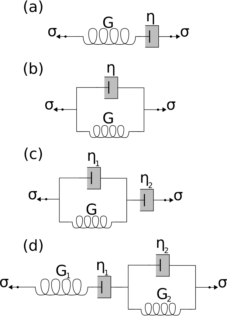
Figure 4: Sketch of some mechanical models of viscoelastic fluids that are built from elastic elements (denoted with their Young’s modulus $G$) and viscous elements (denoted with their viscosity $\eta$) combined in series or in parallel, and to which a stress $\sigma$ is applied. (a) Maxwell model. (b) Kelvin–Voigt model. (c) Jeffreys model. (d) Burgers model.

Viscoelastic materials are not-Newtonian fluids, that is, they do not obey Eq. (3). The Newtonian expression works remarkably well for simple liquids composed of small, roughly isotropic molecules. This happens because of a separation of times scales: the molecular relaxation time is comparable to the time to diffuse one molecular length, which is $\tau_{0}\approx\ell^{2}/D\approx 10^{-13}$ s. The flow velocity can interfere with these relaxation times only in exceptional cases. Consider now a complex fluid comprised of elongated, flexible molecules that possibly form links with each others. The molecular relaxation time is now much larger, and can be matched by realistic shear rates. One is naturally led to define a dimensionless number comparing these time scales, the so-called Weissenberg number $\mathcal{W}\equiv\tau_{0}\dot{\gamma}$, where $\dot{\gamma}$ is the shear rate. When $\mathcal{W}\ll 1$ one recovers a Newtonian fluid; but for $\mathcal{W}\gtrsim 1$ the shear rate interferes with the molecular relaxation, and therefore one should expect nonlinear or history-dependent terms in the constitutive equation for the stress tensor.

We now discuss the basic physical concepts necessary to describe the viscoelastic behavior of biofilms (see  joseph2013 ; morozov2015 for more details). Any material responds with a deformation $\gamma$ to an applied stress $\sigma$ (force per unit area). For an elastic solid $\sigma=G\gamma$, where $G$ is the elastic modulus; for a liquid $\sigma=\eta\tfrac{\partial\gamma}{\partial t}$, where $\eta$ is the viscosity. A viscoelastic material must combine both elastic and viscous response. The simplest physical model thereof is the Maxwell element where an elastic spring and a viscous dashpot are combined in series (see Fig. 4(a)). For simplicity we consider at first a one-dimensional problem. For this configuration the stresses on the two elements are equal $\sigma=\sigma_{1}=\sigma_{2}$ and the deformations are additive, hence $\tfrac{\partial\gamma}{\partial t}=\tfrac{\partial\gamma_{1}}{\partial t}+\tfrac{\partial\gamma_{2}}{\partial t}=\tfrac{1}{G}\tfrac{\partial\sigma}{\partial t}+\tfrac{\sigma}{\eta}$. The constitutive equation for the Maxwell model is then

$$\lambda\frac{\partial\sigma}{\partial t}+\sigma=\frac{\partial\gamma}{\partial t}\,,$$ (21)

where $\lambda\equiv\eta/G$ is a relaxation time. The formal solution of Eq. (21) is

$$\sigma(t)=\frac{1}{\lambda}\int_{-\infty}^{t}e^{-\frac{t-t^{\prime}}{\lambda}}\eta\frac{\partial\gamma}{\partial t^{\prime}}\mathrm{d}t^{\prime}\,.$$ (22)

While for time scales much shorter than the relaxation ($\lambda\to\infty$) one finds solid-like behavior ($\sigma=G\gamma$), for observation times much larger than the relaxation ($\lambda\to 0$) one finds viscous behavior ($\sigma=\eta\tfrac{\partial\gamma}{\partial t}$). The Maxwell model then behaves as a fluid, and therefore is not suitable for a real viscoelastic material.

Another, historically important, model is the Kelvin–Voigt element, where the spring and dashpot are arranged in parallel (see Fig. 4(b)). The Kelvin–Voigt constitutive equation is

$$\sigma=G\gamma+\eta\frac{\partial\gamma}{\partial t}\,.$$ (23)

At long observation times the Kelvin–Voigt material behaves solid-like because it always returns to its equilibrium configuration.

We can improve our model of viscoelastic materials by adding a dashpot in series with a Kelvin–Voigt element, producing the Jeffreys model (see Fig. 4(c)). The strains in the dashpot and in the Kelvin–Voigt element are additive, $\tfrac{\partial\gamma}{\partial t}=\tfrac{\partial\gamma_{1}}{\partial t}+\tfrac{\partial\gamma_{2}}{\partial t}$, and the stresses are $\sigma=\eta_{1}\tfrac{\partial\gamma_{1}}{\partial t}=G\gamma_{2}+\eta_{2}\tfrac{\partial\gamma_{2}}{\partial t}$. Solving for the total strain $\gamma$ and total stress $\sigma$, one finds the constitutive equation

$$\lambda_{1}\frac{\partial\sigma}{\partial t}+\sigma=\eta_{1}\left(\frac{\partial\gamma}{\partial t}+\lambda_{2}\frac{\partial^{2}\gamma}{\partial t^{2}}\right),$$ (24)

where $\lambda_{1}\equiv\left(\tfrac{\eta_{1}+\eta_{2}}{G}\right)$ is a relaxation time and $\lambda_{2}\equiv\tfrac{\eta_{2}}{G}$ a retardation time. We can obtain a more general equation by considering the deformation field $\xi(x,t)$ and by realizing that $\tfrac{\partial\gamma}{\partial t}=\tfrac{\partial}{\partial t}\tfrac{\partial\xi(x,t)}{\partial x}=\frac{\partial v}{\partial x}$, that is the velocity gradient or rate-of-strain tensor. In three dimensions, it is $\nabla\vec{v}$. Remembering that $\bm{\sigma}=-p\bm{\mathrm{I}}+\bm{\tau}$ (see Sec. II.1), the Jeffreys constitutive equation then becomes

$$\lambda_{1}\frac{\partial\bm{\tau}}{\partial t}+\bm{\tau}=2\eta_{1}\left(\mathbf{D}[\vec{v}]+\lambda_{2}\frac{\partial\mathbf{D}[\vec{v}]}{\partial t}\right)\,,$$ (25)

where $\mathbf{D}[\vec{v}]\equiv\tfrac{1}{2}\left(\nabla\vec{v}+\nabla\vec{v}^{\mathrm{T}}\right)$ is the symmetric part of the rate-of-strain tensor. The formal solution of Jeffreys constitutive equation is

$$\bm{\tau}=2\eta_{1}\frac{\lambda_{2}}{\lambda_{1}}\mathbf{D}[\vec{v}]+2\frac{\eta_{1}}{\lambda_{1}}\!\left(1-\frac{\lambda_{2}}{\lambda_{1}}\right)\!\int_{-\infty}^{t}e^{\frac{t-t^{\prime}}{\lambda_{1}}}\mathbf{D}[\vec{v}]\mathrm{d}t^{\prime}.$$ (26)

The Maxwell model is recovered when $\lambda_{2}=0$, and the Newtonian fluid when $\lambda_{1}=\lambda_{2}$.

Another way of dealing with the rheology of non-Newtonian fluids is to assume that only the rate of dissipation in the fluid changes but not the structure of the stress tensor. One then writes

$$\bm{\sigma}=-p\bm{\mathrm{I}}+\eta(\mathbf{D}[\vec{v}])\mathbf{D}[\vec{v}]\,.$$ (27)

Because the viscosity cannot change for a change of coordinate system (must be invariant), $\eta(\mathbf{D}[\vec{v}])$ must be a function of the tensorial invariants build with $\mathbf{D}[\vec{v}]$. The lowest order term is $\dot{\gamma}^{2}\equiv\tfrac{1}{2}\mathbf{D}:\mathbf{D}$. The rheology of the material is then governed by the properties of the function $\eta(\dot{\gamma})$. If $\frac{\partial\eta}{\partial\dot{\gamma}}>0$ the fluid is called shear-thickening, that is, it becomes increasingly stiffer as the shear-rate increases; if $\frac{\partial\eta}{\partial\dot{\gamma}}<0$ the fluid is called shear-thinning, that is the material becomes less viscous as the shear-rate increases.

Experimentally, a common rheological technique to characterize viscoelastic materials is the measurement of the stress-strain curve. The sample is subject to a shear stress which increases monotonically with time up to a maximum value; this corresponds to the “loading” phase. Subsequently, the shear stress is decreased; this is the “unloading” phase. The presence of hysteresis is characteristic of viscous dissipation in the material. Another common rheological technique is the creep test, where a stress is applied for a prolonged interval of time and then suddenly released. The temporal evolution of the strain exhibits characteristic regions corresponding to different processes taking place: (i) an instantaneous elastic stretching, (ii) a viscous flow, (iii) after the external stress ceases there is an instantaneous elastic recoil, (iv) a time-dependent creep recovery stoodleyJIndMBBiotech2002 .

The experimental investigation of biofilms’ material properties is still in an early stage, and different models are proposed to explain the experimental data. For example, the biofilms of different Pseudomonas aeruginosa strains were subject to strain and creep tests and the results were fitted with a Jeffreys model that includes a slow nonlinearity to account for the shear-thickening behavior klapperBiotechBioeng2002 . That theory correctly predicts the relaxation time at high shear rates. However, the biofilm of Streptococcus mutans (common in dental plaque) showed creep compliance consistent with a Burgers model vinogradovBiofilms2004 (see Fig. 4(d)). Biofilms vary greatly in their composition and structure. The biofilm of Streptococcus mutans appears to be shear-thinning vinogradovBiofilms2004 ; cheongRheolActa2009 ; the biofilms of the microalga Chlorella vulgaris also shows shear-thinning behavior  wilemanBioresTech2012 . Pseudomonas aeruginosa builds instead a shear-thickening biofilm klapperBiotechBioeng2002 . Therefore, it should not be surprising that measurements based on creep tests of $44$ biofilms determined values of $G$ and $\eta$ spanning eight decades shawPRL2004 . However, they also found a remarkably small range of variability for the elastic relaxation time $\lambda\approx\eta/G$, with an average of $18$ min shawPRL2004 . It is argued that this common relaxation time can hardly be a coincidence, but rather a sign of convergent evolution. The time scale $\lambda$ separates the solid-like from the liquid-like behavior of a biofilm. Short mechanical stresses can be absorbed by an elastic response, but a sustained stress can be deleterious as it could lead to structural failure, The biofilm reacts instead as a viscous fluid for long time-scale stresses. The time scale of $18$ min coincides with the time required to elicit a phenotypic response at the cellular level vandykApplEnvMB1994 ; ptitsynApplEnvMB1997 , which is however expensive in terms of cellular resources. Thus, the elastic relaxation time needs to be large enough to avoid unnecessary response to intermittent stresses, but smaller or approximately equal to the biological time to initiate expensive genetically-regulated responses shawPRL2004 .

A biofilm growing under flow conditions develops characteristic elongated, filamentous structures called streamers (see Fig. 2(b), (e) and (g)). They are ubiquitous in natural environments and strongly influence flow through porous materials, medical and industrial devices rusconiInterface2010 ; rusconiBiophysJ2011 ; drescherPNAS2013 . As the EPS network of streamers percolates through the channels or pores more and more planktonic cells are caught within it. Eventually, the streamers lead to a catastrophic clogging of the pores that stops the flow drescherPNAS2013 . Biofilms grown up to Reynolds numbers of $\mathcal{R}=3600$ produced streamers that behaved as viscoelastic solids for stresses lower than the value at which they were grown, but behaved like viscoelastic fluids at larger stresses stoodleyBiotechBioeng1999 ; stoodleyJIndMBBiotech2002 , that is similar to a Bingham fluid. In the linear regime streamers exhibited a shear modulus of $27$ N/m² and a Young modulus in the range of $17$ to $40$ N/m² stoodleyBiotechBioeng1999 .

Strong flow conditions, in the turbulent regime, produce ripple structures in mixed species biofilms that migrate with a speed of $800~{}\mu$m/h stoodleyEnvMB1999 . At $\mathcal{R}=4200$ the ripples have a wavelength of about $75~{}\mu$m, but it increases to about $200~{}\mu$m at $\mathcal{R}=1200$. The ripples moves downstream, which points at an important effect for surface colonization. Furthermore the morphology of the ripples responded within minutes to changes in the flow velocity. This fact indicates that the formation of ripples must have a hydrodynamical origin. Indeed, recent work  thomasPhilTransRoySocLond2013 on fossilized microbial mats called Kinneyia confirms this. Kinneyia are sedimentary fossils characterized by ripples with wavelength between $2$ and $20$ mm. Theory and experiments using an artificial biofilm shows that the rippled structures can be explained by the ancient flowing of water above the mats that produced a Kelvin–Helmholtz instability thomasPhilTransRoySocLond2013 . This hydrodynamic instability occurs at the interface between two fluids with different viscosities and flowing with different velocities and produces ripples with wavelength proportional to the thickness of the biofilm. This theory predicts morphologies, wavelengths and amplitudes consonant with the fossil samples thomasPhilTransRoySocLond2013 .

Two important challenges have been identified for future investigations of biofilms from the point of view of rheology and complex fluids billingsRepPrgPhys2015 : (i) the structure and morphology of biofilms depend on their history of growth and on the substratum; for example, the biofilm of Pseudomonas aeruginosa growing in human lungs and airways incorporates DNA and the F-actin protein walkerInfImm2005 , which modify the material properties of the biofilm with respect to a lab-grown sample. The thickness of the in vivo biofilm of the fungus Candida albicans is up to four times larger than the in vitro biofilm andesInfImm2004 . (ii) An integrated model of the biofilm’s material properties should guide the understanding of its development and also of its dissolution, which is crucial in clinical settings. Helpful in this regard can be investigations of hydrogels (which are cross-linked networks of hydrophilic polymers) because these well-studied systems can illuminate different aspects of the biofilm’s physics. For example, physical models for the diffusion of macromolecules within gels phillipsAICHEJ1989 ; masaroProgPolySci1999 ; amsdenMacromol1998 can instruct the understanding of biomolecules regulating the biofilm growth and the mechanism of drug delivery to destroy it. Self-healing polymeric materials woolSoftMatt2008 ; wuProgPolymSci2008 can be a guide to biofilms as adaptive materials. More progress is expected from the comparison with highly controllable artificial systems stewartSciRep2015 .

V Integrated Experimental Methods

Biofilms are complex systems as they have characteristic length and time scales spanning many orders of magnitude but that crucially interact with each other in a hierarchical way, and produce robust order simon1991 . At the nanometer scale molecular processes such as gene expression, biosynthesis and the activity of the signal transduction networks take place. At the micrometer scale flagellar and ciliar motion governs the motility of the cells; diffusion of nutrients, and gradients in the chemoattractants and quorum sensing cues shape the average behavior of a group of cells. At larger scales hundreds of microorganisms form aggregates held together by pili and EPS; they form ripples and streamers under the influence of hydrodynamic forces. The biofilm undergoes stages of maturation and dispersal, while some cells revert to the motile phenotype and colonize new surfaces morgenrothRevEnvSciBiotech2009 . An understanding of the biofilm state must then integrate these different length and time scales involved.

Different “integrated”, experimental approaches have already emerged. Microfluidic and lab-on-a-chip devices offer the possibility to include several functions in a microscopic environment, offer high throughput, and length and time scales compatible with the ecological conditions of biofilms vertesAnalChem2012 ; karimiLOC2015 . For example, microfluidic devices which mimics xylem vessels were used to measure the adhesion forces of type I and type IV pili for Xylella fastidiosa delafuente2007 , or to characterize the adhesion, motility and biofilm formation of Acidovorax citrulli baharFEMSMBLett2010 . A nanoporous microfluidic platform was used to determine the amount of acetic acid necessary to impair the motility of Listeria monocytogenes wrightLabChip2014 . The biofilm growth and dispersal dynamics of Staphylococcus epidermidis was investigated with a microfluidic device that allows to control the local hydrodynamic conditions leeBiomedDev2008 . A microfluidic assay was used to develop an in situ analytical system to assay the susceptibility of biofilms to antibiotics kimLabChip2010 . Microsensors and microfluidics were employed to monitor phenotypic responses of fungal biofilms to changes in shear stress and antifungal drugs richterLabChip2007 . A microfluidic biofilm signaling circuit that uses a population-driven quorum sensing switch can form or displace consortia of fungal biofilms hongNatCom2012 . This platform allows for non-invasive, robust continuous monitoring of the biofilm conditions. Microfabricated elastomer chips allow to monitor and study the evolution of bacterial and yeast colonies in a chemically controlled, dynamic environment groismanNatMeth2005 . The architecture of the device resembles the complex structures naturally produced by biofilms, that is, clusters of cells separated by channels along which nutrients and waste products flow. A microfluidic porous device demonstrated that the formation of streamers takes place only in a certain flow rate range, and that streamers act as precursors to structures found in biofilm growing in porous media valiei2LabChip012 . A microfluidic devices that incorporates a microbial fuel cell was used to generate electricity and may find application as a small-scale biosensing device that offers great flexibility because of its lab-on-a-chip technology liBiotechBioeng2011 . The bacteria used to produce power were the exoelectrogenic Geobacter sulfurreducens and Shewanella oneidensis. These Gram-negative bacteria have the capability to exchange electrons with soluble and insoluble electron acceptors as part of their respiratory chain nealsonAnnRevMB1994 ; gorbyPNAS2006 . Recently, a novel method that combines surface enhanced Raman spectroscopy and confocal Raman spectroscopy (SECRaM) was developed schkolnikPLOS2015 . This method allows the in situ spatial and temporal, analytic investigation of Shewanella oneidensis biofilms without disturbing it.

Nanofabrication and microfluidics are excellent tools for manipulating the cells’ microenvironment and monitor their responses weibelNAtRevMB2007 ; holScience2014 ; rusconiAnnRevBiophys2014 . By using surfaces with a pattern of micropillars it was shown that Escherichia coli bacteria use their flagella to reach inside the crevices between pillars and adhere to them when the spacing of the pillars is smaller than the cell size friedlanderPNAS2013 . Thus, it was shown that flagella in addition to swimming motility create a dense fibrous network that gives structural stability to biofilms friedlanderPNAS2013 . Microfluidic methods revealed that there is an underlying hydrodynamic mechanism that produces streamers, that is, the secondary vortical motion that is very pronounced around corners rusconiInterface2010 ; rusconiBiophysJ2011 ; drescherPNAS2013 .

Nanofabricated devices have the potential to unravel the complex structural organization of bacterial populations in natural environments, which are chemically and physically heterogeneous. Biofilms commonly contain more than one species, and therefore both cooperation and competition shape the community in dynamic states of organization. Aspects of biofilm sociobiology nadellFEMSMBRev2009 are now within the grasp of experimental testing. Escherichia coli colonizing an array of microhabitat patches formed a “metapopulation”, that is a population of populations, that adapts quickly to habitats with high niche diversity keymerPNAS2006 . Well-defined microscale spatial structures are a necessary and sufficient condition for the stability of bacterial communities engaged in “reciprocal syntrophy”, that is a partition of functions all necessary for the survival of the whole community kimPNAS2008 . Thus, the local topography is a crucial factor to account for in the biofilm’s growth and viability. There are also efforts to move to three dimensions. A three-dimensional (3D) printing technique was used to study the cell-cell interactions in structured 3D environments that model bacterial aggregates in the human body connellPNAS2013 , for example. It was found that Staphylococcus aureus, whose mono-species colonies are susceptible to ampicillin, is granted resistance to it by a community of Pseudomonas aeruginosa forming a shell around it connellPNAS2013 . However, much still remains to be understood, as it appears that subtle details often determine the fate of the colony holBMCResNot2015 .

These bottom-up approaches aimed at recreating the complex ecological landscape of bacterial communities in a controlled manner hold the promise to illuminate the behavior of single cells and the dynamical organization occurring in a biofilm. Similarly to the revolution in information technology brought forth by the miniaturization of semiconductor electronics, the fields of microfluidics and nanofabrication may usher a new level of understanding of microbiology.

VI Theoretical and Computational Methods

Theoretical models of biofilm growth and dynamics have started since the 1970s with simple one-dimensional differential equations describing a flat layer. In the following we will start by reviewing the basic concepts of that early era that originated from models of bacterial cultures herbertJGenMB1956 ; vanUden1967 because, although our understanding of biofilms has advanced since then, these ideas and equations are still a part of the more complex models and methods considered in the modern scientific debate.

Consider a colony of microorganisms in a well-mixed bath of substrate (for example in a continuous culture apparatus). The specific growth rate of the colony $\mu$ is written as $\mu=\tfrac{1}{c}\tfrac{\mathrm{d}c}{\mathrm{d}t}=\frac{\mathrm{d}}{\mathrm{d}t}\ln c$ where $c$ is the concentration of cells. Monod monod1942 famously related $\mu$ to the concentration $s$ of an essential growth substrate

$$\mu=\mu_{m}\left(\frac{s}{K_{s}+s}\right),$$ (28)

where $\mu_{m}$ is the growth rate constant and $K_{s}$ is the saturation constant, that is, the substrate concentration at which $\mu=\frac{1}{2}\mu_{m}$. The growth rate is proportional to the substrate concentration when $s\ll K_{s}$, but it saturates at large values of $s$, $s\gg K_{s}$. A second fundamental law of Monod relates the growth rate to the substrate consumption rate

$$\frac{\mathrm{d}c}{\mathrm{d}t}=-Y\frac{\mathrm{d}s}{\mathrm{d}t},$$ (29)

where $Y$ is the yield constant, the ratio of mass of cells grown and mass of substrate used. Combining Eq. (29) with the definition of $\mu$ yields the basic equations

$$\frac{\mathrm{d}s}{\mathrm{d}t}=-kc\frac{s}{K_{s}+s}\,,\quad\frac{\mathrm{d}c}{\mathrm{d}t}=\mu_{m}c\frac{s}{K_{s}+s}$$ (30)

where $k\equiv\mu_{m}/Y$ is the maximum specific rate of substrate consumption.

Consider now a biofilm immersed in a bulk liquid. For simplicity we assume a biofilm growing on a flat surface that we take as the $xy$-plane and with a $z$-axis normal to it. The substrate, that is, the energy source diffuses from the surface of the biofilm to the deeper layers, and its concentration decays with depth. Thus, there is an additional term in the balance equation for $s$ due to molecular diffusion

$$\frac{\mathrm{d}s}{\mathrm{d}t}=-k\frac{cs}{K_{s}+s}+D_{s}\frac{\partial^{2}s}{\partial z^{2}}\,,$$ (31)

where $D_{s}$ is the diffusivity of substrate within the biofilm. A biofilm is considered in a steady state if the total biomass is equal to what can be sustained by the flux of substrate rittmannBiotechBioeng1980 . It is a statement of conservation of energy. In a steady state, the net biofilm growth rate of cells is rittmannBiotechBioeng1980

$$\frac{\mathrm{d}c}{\mathrm{d}t}=\mu_{m}c\left(\frac{s}{K_{s}+s}\right)-bc\,,$$ (32)

where $b$ is the specific decay coefficient.

This and similar approaches kisselJEnvEng1984 ; wannerBiotechBioeng1986 ; chaudhryChemEng1998 viewed biofilms as simple flat structures, governed by energy balance considerations. However, the development of techniques such as confocal scanning laser microscopy revealed that biofilms have a heterogeneous spatial structure interspersed with channels and chambers lawrenceJBact1991 ; costertonARMB1995 . Thus, the next step in the mathematical modeling of biofilm was the fully 3D description and the inclusion of a diffusive mechanism for biomass spreading with a diffusion coefficient that depends nonlinearly on the biomass concentration. Eberl et al. eberlJTheoMed2001 proposed the equations

$$\nabla\cdot\vec{v}=0\,,\quad\frac{\partial\vec{v}}{\partial t}+\vec{v}\cdot\nabla\vec{v}=-\frac{1}{\rho}\nabla p+\nu\nabla^{2}\vec{v}\,,$$ (33)

$$\frac{\partial s}{\partial t}+\vec{v}\cdot\nabla s=\nabla\cdot\left(D_{1}(c)\nabla s\right)-f(s,c)\,,$$ (34)

$$\frac{\partial c}{\partial t}=\nabla\cdot\left(D_{2}(c)\nabla c\right)+g(s,c)\,,$$ (35)

$$f(s,c)=\frac{k_{1}cs}{k_{2}+s}\,,\quad g(s,c)=k_{3}(f(s,c)-k_{4}c),$$ (36)

where $\vec{v}$ is the flow velocity, $s$ the nutrient concentration, $c$ the biomass density, and $k_{1}\dots k_{4}$ are model parameters. Equations (33) are the Navier–Stokes equations for an incompressible fluid with density $\rho$ and kinematic viscosity $\nu$. Nutrients spread through convection and diffusion and are consumed with a Monod reaction rate $f(s,c)$. The biomass is produced with a rate $g(s,c)$ and spreads through a diffusive flux $D_{2}\nabla c$ (Eq. (35)), where $D_{2}(c)=(\frac{\epsilon}{c_{max}-c})^{a}c^{b}$. This functional form produces a biomass with a maximum density $c_{max}$, vanishing diffusion for $c\to 0$, and significant biomass spreading only when $c\to c_{max}$. This set of equations are studied for different values of an important dimensionless number $\mathcal{G}$ that quantifies the ratio of the biomass growth rate and substrate transport rate picioreanuBiotechBioeng1998 , and produces heterogeneous, mushroom-like structures similar to what is observed in experiments eberlJTheoMed2001 ; eberlchemEngSc2000 . This approach was generalized to multispecies biofilm with different solutes nogueraWatSciTech1999 .

Experimental results in the mechanics of biofilms stoodleyJIndMBBiotech2002 ; fuxJBacter2004 prompted a phenomenological description of the biofilm mechanics in terms of a multi-fluid model klapperPRE2006 . Consider a biofilm with volume fraction $\phi_{b}$ immersed in a solvent with volume fraction $\phi_{s}$, where $\phi_{s}+\phi_{b}=1$. The fundamental quantity of interest is the cohesion energy functional for the biofilm

$$E[\phi_{b}]=\int\left(f(\phi_{b})+\frac{\kappa}{2}|\nabla\phi_{b}|^{2}\right)\mathrm{d}V,$$ (37)

where $f(\phi_{b})$ is the energy density of the mixing of biomass and solvent, and the gradient term penalizes short-length scale variations by means of a surface energy. The shape of $f(\phi_{b})$ can be deduced from general physical arguments. The function $f(\phi_{b})$ should have a minimum at some volume fraction because the cohesive forces of the biomass are balanced by the short-range repulsions. Because attractive forces are weak at long distance $f(\phi_{b})\to 0$ as $\phi_{b}\to 0$, and because some amount of solvent is necessary, $f(\phi_{b})$ must grow at large $\phi_{b}$. Using mass conservation for the biomass $\frac{\mathrm{d}\phi_{b}}{\mathrm{d}t}+\nabla\cdot(\phi_{b}\vec{u}_{b})=0$ one can write the time derivative of the energy

$$\frac{\mathrm{d}E}{\mathrm{d}t}=-\int\left(\phi_{b}\nabla\cdot\mathbf{\Pi}\right)\cdot\vec{u}_{b}\mathrm{d}V\,,$$ (38)

where $\mathbf{\Pi}=-[f^{\prime}(\phi_{b})-\kappa\nabla^{2}\phi_{b}]\mathbf{I}$ is the cohesive stress tensor, and $\vec{u}_{b}$ the velocity of the biomass. Neglecting the inertial, viscous and viscoelastic terms one finds the evolution equation for $\phi_{b}$ klapperPRE2006 ; klapperSIAMRev2010 ; wangSolStComm2010

$$\frac{\partial\phi_{b}}{\partial t}+\nabla\cdot(\phi_{b}\vec{u}_{b})=\nabla\cdot\left[a(\phi_{b})f^{\prime\prime}(\phi_{b})\nabla\phi_{b}\right]-\\ \kappa\nabla\cdot\left[a(\phi_{b})\nabla\nabla^{2}\phi_{b}\right],$$ (39)

where $a(\phi_{b})=\zeta_{0}^{-1}\phi_{b}(1-\phi_{b})$, and $\zeta_{0}$ is a friction constant. This model was studied in one dimension with $\vec{u}_{b}=0$ (so that Eq. (39) becomes a modified Cahn–Hilliard equation) and a free surface film state is found to form, where spinodal decomposition is a possible mechanism klapperPRE2006 . This approach has been extended to include EPS with an additional phase field, which reproduces the cohesive failure of biofilm under shear flow tierraJRoySocInterf2015 , and with the inclusion of a viscoelastic model of the EPS lindleyPRE2012 .

In contrast to the models based on Eq. (37), a different paradigm of biofilm growth has been proposed, where the biofilm is modeled with stochastic rules that evolve in a discrete way fujikawaJPhysSocJap1989 , as opposed to the continuous changes described by partial differential equations. In these early computational attempts the growth of a bacterial colony was studied matsushitaPhysA1990 ; fujikawaFEMSMBEco1994 ; benNature1994 . For example, experiments on Bacillus subtilis growing on agar plates were compared with three models of stochastic growth: (i) diffusion limited aggregation, (ii) the Eden model, and (iii) the dense branching morphology. Diffusion limited aggregation describes the growth process of small particles in a dilute solution that aggregate when their Brownian trajectories bring them in close contact wittenPRL1981 . Coagulated aerosols or zinc ions in solution, for example, exhibit open, randomly branched structures that can be modeled by diffusion limited aggregation. A simple method to reproduce computationally diffusion limited aggregation is as follows. Consider a 2D square lattice at whose center the first seed is planted; next, a new particle is placed far away from the seed; it then undergoes a random walk on the lattice until it reaches a lattice site neighboring the initial seed, at which point they stick together. The procedure is repeated and new particles stick to the cluster whenever they reach one of its neighboring sites. Alternatively, in the Eden growth model new particles are added next to the perimeter of the cluster eden1961 . When starting from a seed in a planar geometry, compact, disk-like clusters are obtained. Finally, an addition of a kinetic term to the growth process leads to the increase of branching tips as the radius of the agglomerate increases. This process produces the dense branching morphology, which is characterized by compact branches with a neat spherical envelope benPRL1986 ; meakin1998fractals ; stanley2012 . Fujikawa fujikawaFEMSMBEco1994 found that at relative low nutrient concentrations the colony formed open fractal branches, similar to the simulations of diffusion limited aggregation, and measured a fractal dimension $D_{f}=1.73\pm 0.02$ which compares well with known theoretical values hayakawaPRL1997 . For higher nutrient concentrations, the colony grew compact and round, similarly to an Eden cluster, as the cells do not have to rely on the diffusion of nutrients from the surrounding. At low agar concentrations, instead, patterns similar to the dense branching morphology were found, in which case the reduced viscosity allows a growth driven by the flagellar motion.

These stochastic, discrete approaches eventually produced the widely-used class of cellular automata models halleyOikos1994 ; wimpennyFEMSMBEco1997 ; hermanowiczWatSciTech1999 ; picioreanuBiotechBioeng1998 ; picioreanuBiotechBioeng2000 ; pizarroJEnvEng2001 ; tangWatRes2013 . Generally, cellular automata models consider a 2D space partitioned with a lattice. Every lattice location may be occupied by a parcel of biofilm consisting of cells, EPS, and other molecules. Additionally, fields representing nutrients or waste products can also be distributed on the lattice. Each lattice location is updated at discrete time steps according to simple rules. Given a cell in a specific location, the neighboring compartments are searched for empty space, and if the nutrients in that location are sufficient the cell multiplies and occupies that empty location. Nutrients diffuse stochastically through the lattice. More specific rules informed by biological interactions can be implemented. Although cellular automata models appear as a drastic simplification, they can produce complex structures because of their nonlinear nature wolframNature1984 .

A more recent effort at integrating the experimental knowledge about biofilm growth tackles the challenge of modeling its heterogeneous structure and composition laspidouWatRes2004a ; laspidouWatRes2004b . They consider three kinds of solid components (the active biomass of microorganisms, the EPS, and the inert biomass) and three kinds of soluble organic compounds (the bacteria’s limiting donor substrate, and two types of soluble microbial products, which are excreted by cells or released during cell lysis) laspidouWatRes2002b ; laspidouWatRes2002a . The concentrations of all these components evolve in time and space according to partial differential equations that include diffusion, Monod kinetics for the donor substrate, cellular utilization and production, decay of the active biomass and detachment forces. Importantly, biofilm consolidation is included, that is, over time the deeper layers of the biofilm become denser. Coupled to the dynamics of the concentrations of the different biofilm components, the mechanical spreading of active biomass and EPS is implemented through a cellular automata scheme. Once the total density in a compartment exceeds a threshold value, the “mother” cell divides into two “daughter” cells, where one of them moves to a neighboring compartment. Were all neighboring compartments occupied, the daughter cell would push their contents to an unoccupied compartment along the shortest path identified by the algorithm. The threshold density for each compartment grows with time. This fact models the consolidation process due to physical forces acting on the biofilm, for example, hydrodynamic forces tend to induce the solid components to pack more densely.

An alternative class of models considers the individual microbial cell, or small groups thereof, as the elementary computational unit kreftMB1998 ; kreftMB2001 ; kreftWatSciTech2001 ; picioreanuApplEnvMB2004 ; xavierEnvMB2005 ; picioreanuWatSciTech2007 . They differ from cellular automata models as there is no underlying lattice partitioning space. They are called individual-based models, particle-based models, or more generally agent-based models. The same basic rules as the cellular automata models for metabolism, substrate uptake, cell multiplication and death are used but no global rules on the growth are imposed. The advantages of agent based simulations are multiple. First, the absence of a lattice grid avoids artificial results such as fixed growth directions. Second, no global laws (for the growth, e.g.) are prescribed, but must emerge from the microscopic dynamics. Third, cells are modeled as hard spheres, and their overlap produces repulsive forces that induces naturally the spreading of the biofilm. Furthermore, since individual agents are resolved, it is also natural to introduce genetic variability in the cell’s parameters, cell motility picioreanuWatSciTech2007 , coupling with hydrodynamic flow vonderSchulenburgAICHEJ2009 , inclusion of metabolic reactions lardonEnvMB2011 , or a viscous fluid model for the EPS alpkvistBiotechBioeng2006 . However, there are also drawbacks laspidouDesal2010 : for example, the computational cost of this class of models is typically larger than cellular automata’s, and the large-scale structure of biofilm, such as porosity, are less faithfully represented.

VII Conclusions

Biofilms are among the most ancient and most common forms of multicellular organization. They exhibit astounding complexity both at microscopic and mesoscopic length scales. Their importance has been recognized only in recent decades and research in this field is growing tremendously, fueled by the possibility of treating infectious diseases or of benefiting from their appetite for organic materials in wastewater applications.

We have described the main physical processes involved in the inception, growth and dispersal of biofilms. A hydrodynamic description is necessary for the initial transition of microbial cells from the planktonic to the sessile state. Details of the physico-chemical nature of the cellular membrane and its appendages are key for the process of adhesion. Biofilms are macroscopically viscoelastic materials with a very complex, history dependent behavior. Progress in the rheological and mechanical characterization will come from studies in conditions mimicking the natural environment.

We have also reviewed modern experimental techniques of investigation such as microfluidics and lab-on-a-chip technologies that use an integrated approach to biofilms with the aim at capturing their heterogeneous and complex nature. These methods can experimentally “simulate” the natural environment of a biofilm and test different hypotheses. Realistic environments are however essential to understand and control the dispersal of biofilms, for example, which has tremendous consequences for ecology and in the context of infectious diseases. Studies of biofilm dispersal, however, are still largely conducted in vitro kaplanJDentRes2010 .

Finally, we have reviewed the theoretical and computational modeling of biofilms. Computational approaches at simulating a biofilm are now finally coming of age kreftPNAS2013 and some predictions quantitatively match the experimental data, but much remains to be done. Ahead lies a particularly daunting challenge when considering all the chemical, biological and physical processes involved in a biofilm, which evolve and interact from the nanometer to the millimeter length scale, and from the nanosecond time scale to hours or days. Future lines of development should include realistic models for the EPS, either microscopically with a polymer network theory, or mesoscopically with a viscoelastic model. Some attempts are already available alpkvistWatSciTech2007 where the biofilm is modeled with breakable springs in an immersed boundary method, or through a nonlinear, continuum description of worm-like chains ehretJRoySocInterf2013 . Once integrated theoretical and computational models will be developed, they will allow to test and manipulate biofilms under multiple physical, chemical and biological cues, both intrinsic and extrinsic.

We now want to enter a more speculative realm to discuss some mechanisms at play in the biofilm that could be recognized in the future. The important fact that biofilms represent the most complex effort of simple microorganisms at multicellular organization points to the existence of ‘communications’ channels among the individual cells. We know from the biology of multicellular eukaryotes how a complex, well-regulated and specialized structure may exist. Biofilms are more dynamical and history-dependent in their structure and properties. However, interactions that lead to specialization must be there also in biofilms. Obvious candidates are quorum sensing and cell signaling. Although the role of quorum sensing has been linked multiple times with the growth, structure and function of biofilms, controversial results abound (see Ref. parsekTrMB2005 for a critical review of quorum sensing in relation to biofilms). The reason for the controversy is probably the inadequacy of our experimental tools of investigation to the task: more subtle tools for in vivo and in situ analysis are required; another factor that complicates the picture is that the study of mutants elicits the risk of pleiotropy. We speculate that quorum sensing and cell signaling provide the communication channels required to generate complex organization. A second physical aspect that is underrepresented in the study of biofilms is the role of motility. We have reviewed the available evidence on the function of swimming, swarming and twitching within a biofilm. We speculate, however, that these motility modes should have a more important role than currently known. While under some physical forces, such as hydrodynamic shear, a biofilm might respond by forming more compact structures with a sessile population, consortia of different species coexisting, possibly in syntrophic interaction, may utilize motility to assist the spatial segregation often associated with phenotypic differentiation. Biofilms represent still largely unexplored microcosmoses, that will certainly provide numerous surprises in the future.

In this Review, we have omitted the discussion of some crucial aspects in the life-cycle of a biofilm: its ecology and genetic regulation. There is certainly ample space for physical theories of these different levels of interaction.

We gratefully acknowledge Gal Schkolnik for helpful conversations and for critically reading the manuscript. We thank Paul Stoodley for kindly providing the images in Fig. 2.

References

- (1) Noffke N, Christian D, Wacey D and Hazen R M 2013 Astrobiology 13 1103–1124
- (2) Van Kranendonk M J, Philippot P, Lepot K, Bodorkos S and Pirajno F 2008 Precambrian Res. 167 93–124
- (3) Flemming H C and Wingender J 2010 Nat. Rev. Microbiol. 8 623–633
- (4) Hall-Stoodley L, Costerton J W and Stoodley P 2004 Nat. Rev. Microbiol. 2 95–108
- (5) Orell A, Fröls S and Albers S V 2013 Annu. Rev. Microbiol. 67 337–354
- (6) Leadbeater B S C and Callow M E 1992 Formation, composition and physiology of algal biofilms Biofilms – Science and Technology (NATO ASI Series vol 223) ed Melo L F, Bott T R, Fletcher M and Capdeville B (Springer Netherlands) pp 149–162
- (7) Fanning S and Mitchell A P 2012 PLoS Pathog. 8 e1002585
- (8) Ramage G, Mowat E, Jones B, Williams C and Lopez-Ribot J 2009 Crit. Rev. Microbiol. 35 340–355
- (9) Porter J R 1976 Bacteriol. Rev. 40 260
- (10) Henrici A T 1933 J. Bacteriol. 25 277
- (11) Zobell C E 1943 J. Bacteriol. 46 39
- (12) McCoy W F, Bryers J D, Robbins J and Costerton J W 1981 Can. J. Microbiol. 27 910–917
- (13) O’Toole G, Kaplan H B and Kolter R 2000 Annu. Rev. Microbiol. 54 49–79
- (14) Vert M, Hellwich K H, Hess M, Hodge P, Kubisa P, Rinaudo M and Schué F 2012 Pure Appl. Chem. 84 377–410
- (15) Watnick P and Kolter R 2000 J. Bacteriol. 182 2675–2679
- (16) Berk V, Fong J C N, Dempsey G T, Develioglu O N, Zhuang X, Liphardt J, Yildiz F H and Chu S 2012 Science 337 236–239
- (17) Reysenbach A L and Cady S L 2001 Trends Microbiol. 9 79–86
- (18) Taylor C D, Wirsen C O and Gaill F 1999 Appl. Environ. Microbiol. 65 2253–2255
- (19) Wotton R S and Preston T M 2005 BioScience 55 137–145
- (20) Atekwana E A and Slater L D 2009 Rev. Geophys. 47
- (21) Sihorkar V and Vyas S P 2001 Pharm. Res. 18 1247–1254
- (22) Pavithra D and Doble M 2008 Biomed. Mater. 3 034003
- (23) Hao O J, Chen J M, Huang L and Buglass R L 1996 Crit. Rev. Env. Sci. Tec. 26 155–187
- (24) Hamilton W A 1985 Annu. Rev. Microbiol. 39 195–217
- (25) Muyzer G and Stams A J M 2008 Nat. Rev. Microbiol. 6 441–454
- (26) Nicolella C, Van Loosdrecht M C M and Heijnen J J 2000 J. Biotechnol. 80 1–33
- (27) Du Z, Li H and Gu T 2007 Biotechnol. Adv. 25 464–482
- (28) De Beer D and Stoodley P 2013 Microbial biofilms The Prokaryotes ed Rosenberg E, DeLong E, Lory S, Stackebrandt E and Thompson F (Springer Berlin Heidelberg) pp 343–372
- (29) Diels L, van der Lelie N and Bastiaens L 2002 Rev. Env. Sci. Biotechnol. 1 75–82
- (30) Gadd G M 2004 Geoderma 122 109–119
- (31) Sand W, Gerke T, Hallmann R and Schippers A 1995 Appl. Microbiol. Biot. 43 961–966
- (32) Suzuki I 2001 Biotechnol. Adv. 19 119–132
- (33) Bosecker K 1997 FEMS Microbiol. Rev. 20 591–604
- (34) Lawrence J R, Korber D R, Hoyle B D, Costerton J W and Caldwell D E 1991 J. Bacteriol. 173 6558–6567
- (35) Caldwell D E, Korber D R and Lawrence J R 1993 J. Appl. Bacteriol. 74 52S–66S
- (36) Costerton J W, Lewandowski Z, DeBeer D, Caldwell D, Korber D and James G 1994 J. Bacteriol. 176 2137
- (37) Gjaltema A, Arts P A M, Van Loosdrecht M C M, Kuenen J G and Heijnen J J 1994 Biotechnol. Bioeng. 44 194–204
- (38) Stoodley P, Lewandowski Z, Boyle J D and Lappin-Scott H M 1999 Biotechnol. Bioeng. 65 83–92
- (39) Stoodley P, Sauer K, Davies D G and Costerton J W 2002 Annu. Rev. Microbiol. 56 187–209
- (40) Blauert F, Horn H and Wagner M 2015 Biotechnol. Bioeng.
- (41) Madsen J S, Burmølle M, Hansen L H and Sørensen S J 2012 FEMS Immunol. Med. Microbiol. 65 183–195
- (42) Wingender J, Strathmann M, Rode A, Leis A and Flemming H C 2001 Methods Enzymol. 302–14
- (43) Flemming H C, Neu T R and Wozniak D J 2007 J. Bacteriol. 189 7945–7947
- (44) Christensen B E 1989 J. Biotechnol. 10 181–202
- (45) Sutherland I W and Suthe I 1977 Surface Carbohydrates of the Prokaryotic Cell (Academic Press London)
- (46) Sutherland I W 2001 Microbiology 147 3–9
- (47) Wingender J, Neu T R and Flemming H C 2012 Microbial Extracellular Polymeric Substances: Characterization, Structure and Function (Springer Science & Business Media)
- (48) Lawrence J R, Swerhone G D W, Leppard G G, Araki T, Zhang X, West M M and Hitchcock A P 2003 Appl. Environ. Microb. 69 5543–5554
- (49) Ryder C, Byrd M and Wozniak D J 2007 Curr. Opin. Microbiol. 10 644–648
- (50) Colvin K M, Irie Y, Tart C S, Urbano R, Whitney J C, Ryder C, Howell P L, Wozniak D J and Parsek M R 2012 Environ. Microbiol. 14 1913–1928
- (51) Ma L, Jackson K D, Landry R M, Parsek M R and Wozniak D J 2006 J. Bacteriol. 188 8213–8221
- (52) Cooley B J, Thatcher T W, Hashmi S M, L’Her G, Le H H, Hurwitz D A, Provenzano D, Touhami A and Gordon V D 2013 Soft Matter 9 3871–3876
- (53) Donlan R M 2002 Emerg. Infect. Dis. 8 881–890
- (54) Spiers A J, Bohannon J, Gehrig S M and Rainey P B 2003 Mol. Microbiol. 50 15–27
- (55) Götz F 2002 Mol. Microbiol. 43 1367–1378
- (56) Mack D, Fischer W, Krokotsch A, Leopold K, Hartmann R, Egge H and Laufs R 1996 J. Bacteriol. 178 175–183
- (57) Seminara A, Angelini T E, Wilking J N, Vlamakis H, Ebrahim S, Kolter R, Weitz D A and Brenner M P 2012 Proc. Natl. Acad. Sci. USA 109 1116–1121
- (58) Wilking J N, Angelini T E, Seminara A, Brenner M P and Weitz D A 2011 MRS Bull. 36 385–391
- (59) Rubinstein M and Colby R H 2003 Polymer Physics (Oxford University Press, Oxford)
- (60) Or D, Phutane S and Dechesne A 2007 Vadose Zone J. 6 298–305
- (61) Freeman C and Lock M A 1995 Limnol. Oceanogr. 40 273–278
- (62) Norberg A B and Persson H 1984 Biotechnol. Bioeng. 26 239–246
- (63) Teitzel G M and Parsek M R 2003 Appl. Environ. Microbiol. 69 2313–2320
- (64) Hentzer M, Teitzel G M, Balzer G J, Heydorn A, Molin S, Givskov M and Parsek M R 2001 J Bacteriol. 183 5395–5401
- (65) Colvin K M, Gordon V D, Murakami K, Borlee B R, Wozniak D J, Wong G C and Parsek M R 2011 PLoS Pathog. 7 e1001264–e1001264
- (66) Billings N, Ramirez Millan M, Caldara M, Rusconi R, Tarasova Y, Stocker R and Ribbeck K 2013 PLoS Pathog. 9 e1003526
- (67) Wingender J, Jaeger K E and Flemming H C 1999 Interaction between extracellular polysaccharides and enzymes Microbial Extracellular Polymeric Substances (Springer) pp 231–251
- (68) Lock M A, Wallace R R, Costerton J W, Ventullo R M and Charlton S E 1984 Oikos 42 10–22
- (69) Otero A and Vincenzini M 2004 J. Phycol. 40 74–81
- (70) Steinberger R and Holden P 2005 Appl. Environ. Microbiol. 71 5404–5410
- (71) Yang L, Barken K B, Skindersoe M E, Christensen A B, Givskov M and Tolker-Nielsen T 2007 Microbiology 153 1318–1328
- (72) Whitchurch C B, Tolker-Nielsen T, Ragas P C and Mattick J S 2002 Science 295 1487–1487
- (73) Vilain S, Pretorius J M, Theron J and Brözel V S 2009 Appl. Environ. Microbiol. 75 2861–2868
- (74) Mulcahy H, Charron-Mazenod L and Lewenza S 2008 PLoS Pathog. 4 e1000213
- (75) Ahimou F, Jacques P and Deleu M 2000 Enzyme Microb. Tech. 27 749–754
- (76) Irie Y, O’toole G A and Yuk M H 2005 FEMS Microbiol. Lett. 250 237–243
- (77) Rodrigues L R, Banat I M, Mei H C, Teixeira J A and Oliveira R 2006 J. Appl. Microbiol. 100 470–480
- (78) Rivardo F, Turner R J, Allegrone G, Ceri H and Martinotti M G 2009 Appl. Microbiol. Biot. 83 541–553
- (79) Romaní A M, Fund K, Artigas J, Schwartz T, Sabater S and Obst U 2008 Microb. Ecol. 56 427–436
- (80) Zhang X and Bishop P L 2003 Chemosphere 50 63–69
- (81) Elkins J G, Hassett D J, Stewart P S, Schweizer H P and McDermott T R 1999 Appl. Environ. Microb. 65 4594–4600
- (82) Barondes S H 1984 Science 223 1259–1264
- (83) Diggle S P, Stacey R E, Dodd C, Cámara M, Williams P and Winzer K 2006 Environ. Microb. 8 1095–1104
- (84) Pérez-Giménez J, Mongiardini E J, Althabegoiti M J, Covelli J, Quelas J I, López-García S L and Lodeiro A R 2009 Int. J. Microbiol. 2009 719367
- (85) Karatan E and Watnick P 2009 Microbiol. Mol. Biol. R. 73 310–347
- (86) Sauer K, Cullen M C, Rickard A H, Zeef L A H, Davies D G and Gilbert P 2004 J Bacteriol. 186 7312–7326
- (87) Boles B R, Thoendel M and Singh P K 2005 Mol. Microbiol. 57 1210–1223
- (88) Jackson D W, Suzuki K, Oakford L, Simecka J W, Hart M E and Romeo T 2002 Journal of bacteriology 184 290–301
- (89) McDougald D, Rice S A, Barraud N, Steinberg P D and Kjelleberg S 2012 Nat. Rev. Microbiol. 10 39–50
- (90) Crespi B J 2001 Trends Ecol. Evol. 16 178–183
- (91) Shapiro J A 1998 Annu. Rev. Microbiol. 52 81–104
- (92) Ben-Jacob E, Cohen I and Levine H 2000 Adv. Phys. 49 395–554
- (93) Kaplan J B 2010 J. Dent. Res. 89 205–218
- (94) Teschler J K, Zamorano-Sánchez D, Utada A S, Warner C J A, Wong G C L, Linington R G and Yildiz F H 2015 Nat. Rev. Microbiol. 13 255–268
- (95) Sauer K, Camper A K, Ehrlich G D, Costerton J W and Davies D G 2002 J. Bacteriol. 184 1140–1154
- (96) Tolker-Nielsen T, Brinch U C, Ragas P C, Andersen J B, Jacobsen C S and Molin S 2000 J. Bacteriol. 182 6482–6489
- (97) Barken K B, Pamp S J, Yang L, Gjermansen M, Bertrand J J, Klausen M, Givskov M, Whitchurch C B, Engel J N and Tolker-Nielsen T 2008 Environ. Microbiol. 10 2331–2343
- (98) Vlamakis H, Aguilar C, Losick R and Kolter R 2008 Genes Dev. 22 945–953
- (99) Henrichsen J 1972 Bacteriol Rev. 36 478
- (100) Turner L, Ryu W S and Berg H C 2000 J. Bacteriol. 182 2793–2801
- (101) Berg H C 2008 Curr. Biol. 18 R689–R691
- (102) Parkinson J S 1993 Cell 73 857–871
- (103) Block S M, Blair D F and Berg H C 1989 Nature 338 514–518
- (104) Berg H C 2003 Ann. Rev. Biochem. 72 19
- (105) Lauga E and Powers T R 2009 Rep. Prog. Phys. 72 096601
- (106) Koch D L and Subramanian G 2011 Annu. Rev. Fluid Mech. 43 637–659
- (107) Happel J and Brenner H 2012 Low Reynolds Number Hydrodynamics: with special applications to particulate media (Springer Science & Business Media)
- (108) Copeland M F and Weibel D B 2009 Soft Matter 5 1174–1187
- (109) Guyon E, Hulin J P, Petit L and Mitescu C D 2001 Physical Hydrodynamics (Springer, Berlin Heidelberg, New York)
- (110) Purcell E M 1977 Am. J. Phys 45 3–11
- (111) Baskaran A and Marchetti M C 2009 Proc. Natl. Acad. Sci. USA 106 15567–15572
- (112) Simha R A and Ramaswamy S 2002 Phys. Rev. Lett. 89(5) 058101
- (113) Saintillan D and Shelley M J 2007 Phys. Rev. Lett. 99(5) 058102
- (114) Kessler J O and Wojciechowski M F 1997 Collective behavior and dynamics of swimming bacteria Bacteria as multicellular organisms ed Shapiro J A and Dworkin M (Oxford University Press) pp 417–450
- (115) Dombrowski C, Cisneros L, Chatkaew S, Goldstein R E and Kessler J O 2004 Phys. Rev. Lett. 93(9) 098103
- (116) Sokolov A and Aranson I S 2012 Phys. Rev. Lett. 109 248109
- (117) Dunkel J, Heidenreich S, Drescher K, Wensink H H, Bär M and Goldstein R E 2013 Phys. Rev. Lett. 110 228102
- (118) Zöttl A and Stark H 2014 Phys. Rev. Lett. 112 118101
- (119) Wensink H H, Dunkel J, Heidenreich S, Drescher K, Goldstein R E, Löwen H and Yeomans J M 2012 Proc. Natl. Acad. Sci. USA 109 14308–14313
- (120) Drescher K, Dunkel J, Cisneros L H, Ganguly S and Goldstein R E 2011 Proc. Natl. Acad. Sci. USA 108 10940–10945
- (121) Lushi E, Wioland H and Goldstein R E 2014 Proc. Natl. Acad. Sci. USA 201405698
- (122) Katz D F 1974 J. Fluid Mech. 64 33–49
- (123) Brennen C and Winet H 1977 Annu. Rev. Fluid Mech. 9 339–398
- (124) DiLuzio W R, Turner L, Mayer M, Garstecki P, Weibel D B, Berg H C and Whitesides G M 2005 Nature 435 1271–1274
- (125) Kudo S, Imai N, Nishitoba M, Sugiyama S and Magariyama Y 2005 FEMS Microbiol. Lett. 242 221–225
- (126) Magariyama Y, Ichiba M, Nakata K, Baba K, Ohtani T, Kudo S and Goto T 2005 Biophys. J. 88 3648–3658
- (127) Li G, Tam L K and Tang J X 2008 Proc. Natl. Acad. Sci. USA 105 18355–18359
- (128) Rothschild L 1963 Nature 198 1221
- (129) Cosson J, Huitorel P and Gagnon C 2003 Cell Motil. Cytoskel. 54 56–63
- (130) Berke A P, Turner L, Berg H C and Lauga E 2008 Phys. Rev. Lett. 101 038102
- (131) Blake J R and Chwang A T 1974 J. Eng. Math. 8 23–29
- (132) Kearns D B 2010 Nature Rev. Microbiol. 8 634–644
- (133) Darnton N C, Turner L, Rojevsky S and Berg H C 2010 Biophys. J. 98 2082–2090
- (134) Shinoda S and Okamoto K 1977 Journal of bacteriology 129 1266–1271
- (135) McCarter L 1999 J Mol. Microbiol. Biotechnol. 1 51–57
- (136) Merino S, Shaw J G and Tomás J M 2006 FEMS Microbiol. Lett. 263 127–135
- (137) Gavin R, Rabaan A A, Merino S, Tomás J M, Gryllos I and Shaw J G 2002 Mol Microbiol. 43 383–397
- (138) Kirov S M, Tassell B C, Semmler A B T, O’Donovan L A, Rabaan A A and Shaw J G 2002 J. Bacteriol. 184 547–555
- (139) Jones H E and Park R W A 1967 J. Gen. Microbiol. 47 369–378
- (140) Harshey R M 2003 Ann. Rev. Microbiol. 57 249–273
- (141) Kearns D B and Losick R 2003 Mol. Microbiol. 49 581–590
- (142) Julkowska D, Obuchowski M, Holland I B and Séror S J 2005 Journal of bacteriology 187 65–76
- (143) Lindum P W, Anthoni U, Christophersen C, Eberl L, Molin S and Givskov M 1998 J. Bacteriol. 180 6384–6388
- (144) Eberl L, Molin S and Givskov M 1999 J. Bacteriol. 181 1703–1712
- (145) Copeland M F, Flickinger S T, Tuson H H and Weibel D B 2010 Appl. Environ. Microbiol. 76 1241–1250
- (146) Morrison R B and Scott A 1966 Nature 211 255–257
- (147) Jones B V, Young R, Mahenthiralingam E and Stickler D J 2004 Infect. Immun. 72 3941–3950
- (148) Zhang H P, Be’er A, Florin E L and Swinney H L 2010 Proc. Natl. Acad. Sci. USA 107 13626–13630
- (149) Bonabeau E, Dagorn L and Fréon P 1999 Proc. Natl. Acad. Sci. USA 96 4472–4477
- (150) Narayan V, Ramaswamy S and Menon N 2007 Science 317 105–108
- (151) Das D, Das D and Prasad A 2012 J. Theor. Biol. 308 96–104
- (152) Shimada H, Ikeda T, ichi Wakita J, Itoh H, Kurosu S, Hiramatsu F, Nakatsuchi M, Yamazaki Y, Matsuyama T and Matsushita M 2004 J. Phys. Soc. Japan 73 1082–1089
- (153) Hiramatsu F, Wakita J i, Kobayashi N, Yamazaki Y, Matsushita M and Matsuyama T 2005 Microbes Environ. 20 120–125
- (154) Arouh S 2001 Phys. Rev. E 63 031908
- (155) Czirók A, Matsushita M and Vicsek T 2001 Phys. Rev. E 63 031915
- (156) Golding I, Kozlovsky Y, Cohen I and Ben-Jacob E 1998 Physica A 260 510–554
- (157) Wakano J Y, Maenosono S, Komoto A, Eiha N and Yamaguchi Y 2003 Phys. Rev. Lett. 90 258102–258102
- (158) Ben-Jacob E, Cohen I, Czirók A, Vicsek T and Gutnick D L 1997 Physica A 238 181–197
- (159) Ben-Jacob E, Schochet O, Tenenbaum A, Cohen I, Czirok A and Vicsek T 1994 Nature 368 46–49
- (160) Ben-Jacob E, Cohen I, Shochet O, Tenenbaum A, Czirók A and Vicsek T 1995 Phys. Rev. Lett. 75 2899
- (161) Wensink H H and Löwen H 2012 J. Phys.: Condens. Matter 24 464130
- (162) Shrout J D, Chopp D L, Just C L, Hentzer M, Givskov M and Parsek M R 2006 Mol. Microbiol. 62 1264–1277
- (163) Verstraeten N, Braeken K, Debkumari B, Fauvart M, Fransaer J, Vermant J and Michiels J 2008 Trends Microbiol. 16 496–506
- (164) Parsek M R and Greenberg E P 2005 Trends Microbiol. 13 27–33
- (165) Hahn H P 1997 Gene 192 99–108
- (166) Craig L, Pique M E and Tainer J A 2004 Nat. Rev. Microbiol. 2 363–378
- (167) Skerker J M and Berg H C 2001 Proc. Natl. Acad. Sci. USA 98 6901–6904
- (168) Craig L and Li J 2008 Curr. Opin. Struc. Biol. 18 267–277
- (169) Mattick J S 2002 Annu. Rev. Microbiol. 56 289–314
- (170) Merz A J, So M and Sheetz M P 2000 Nature 407 98–102
- (171) Sun H, Zusman D R and Shi W 2000 Curr. Biol. 10 1143–1146
- (172) Maier B, Potter L, So M, Seifert H S and Sheetz M P 2002 Proc. Natl. Acad. Sci. USA 99 16012–16017
- (173) Clausen M, Koomey M and Maier B 2009 Biophys. J. 96 1169–1177
- (174) Clausen M, Jakovljevic V, Søgaard-Andersen L and Maier B 2009 J. Bacteriol. 191 4633–4638
- (175) Holz C, Opitz D, Greune L, Kurre R, Koomey M, Schmidt M A and Maier B 2010 Phys. Rev. Lett. 104 178104
- (176) Conrad J C 2012 Res. Microbiol. 163 619–629
- (177) Müller M J I, Klumpp S and Lipowsky R 2008 Proc. Natl. Acad. Sci. USA 105 4609–4614
- (178) Marathe R, Meel C, Schmidt N C, Dewenter L, Kurre R, Greune L, Schmidt M A, Müller M J I, Lipowsky R, Maier B and Klumpp S 2014 Nat. Comm. 5
- (179) Jin F, Conrad J C, Gibiansky M L and Wong G C 2011 Proc. Natl. Acad. Sci. USA 108 12617–12622
- (180) Gibiansky M L, Conrad J C, Jin F, Gordon V D, Motto D A, Mathewson M A, Stopka W G, Zelasko D C, Shrout J D and Wong G C L 2010 Science 330 197–197
- (181) Conrad J C, Gibiansky M L, Jin F, Gordon V D, Motto D A, Mathewson M A, Stopka W G, Zelasko D C, Shrout J D and Wong G C L 2011 Biophys. J. 100 1608–1616
- (182) Zaburdaev V, Denisov S and Klafter J 2015 Rev. Mod. Phys. 87 483
- (183) Montroll E W and Weiss G H 1965 J. Math. Phys. 6 167–181
- (184) Bouchaud J P and Georges A 1990 Phys. Rep. 195 127–293
- (185) Viswanathan G M, Da Luz M G E, Raposo E P and Stanley H E 2011 The physics of foraging: an introduction to random searches and biological encounters (Cambridge University Press)
- (186) Méndez V, Campos D and Bartumeus F 2013 Stochastic foundations in movement ecology: anomalous diffusion, front propagation and random searches (Springer Science & Business Media)
- (187) Taktikos J, Stark H and Zaburdaev V 2013 PLoS ONE 8 e81936
- (188) Korobkova E, Emonet T, Vilar J M G, Shimizu T S and Cluzel P 2004 Nature 428 574–578
- (189) Burrows L L 2012 Annu. Rev. Microbiol. 66 493–520
- (190) Klausen M, Aaes-Jørgensen A, Molin S and Tolker-Nielsen T 2003 Mol. Microbiol. 50 61–68
- (191) O’Toole G A and Kolter R 1998 Mol. Microbiol. 30 295–304
- (192) Meng Y, Li Y, Galvani C D, Hao G, Turner J N, Burr T J and Hoch H C 2005 J. Bacteriol. 187 5560–5567
- (193) Li Y, Hao G, Galvani C D, Meng Y, De La Fuente L, Hoch H and Burr T J 2007 Microbiology 153 719–726
- (194) Watnick P I and Kolter R 1999 Mol. Microbiol. 34 586–595
- (195) Geiger B, Bershadsky A, Pankov R and Yamada K M 2001 Nat. Rev. Mol. Cell Bio. 2 793–805
- (196) Nan B, Chen J, Neu J C, Berry R M, Oster G and Zusman D R 2011 Proc. Natl. Acad. Sci. USA 108 2498–2503
- (197) Zamir E and Geiger B 2001 J. Cell Sci. 114 3583–3590
- (198) McBride M J 2001 Annu. Rev. Microbiol. 55 49–75
- (199) Mignot T, Shaevitz J W, Hartzell P L and Zusman D R 2007 Science 315 853–856
- (200) Peruani F, Starruß J, Jakovljevic V, Søgaard-Andersen L, Deutsch A and Bär M 2012 Phys. Rev. Lett. 108 098102
- (201) Ginelli F, Peruani F, Bär M and Chaté H 2010 Phys. Rev. Lett. 104(18) 184502
- (202) Peruani F, Deutsch A and Bär M 2006 Phys. Rev. E 74(3) 030904
- (203) Yang Y, Marceau V and Gompper G 2010 Phys. Rev. E 82(3) 031904
- (204) Martínez A, Torello S and Kolter R 1999 J. Bacteriol. 181 7331–7338
- (205) Recht J and Kolter R 2001 J. Bacteriol. 183 5718–5724
- (206) Chen J M, German G J, Alexander D C, Ren H, Tan T and Liu J 2006 J. Bacteriol. 188 633–641
- (207) Wu C w, Schmoller S K, Bannantine J P, Eckstein T M, Inamine J M, Livesey M, Albrecht R and Talaat A M 2009 Microb. Pathogenesis 46 222–230
- (208) Maya-Hoyos M, Leguizamón J, Mariño-Ramírez L and Soto C Y 2015 BioMed Research International 2015 419549
- (209) Davies D G, Chakrabarty A M and Geesey G G 1993 Appl. Environ. Microbiol. 59 1181–1186
- (210) Christensen G D, Simpson W A and Beachey E H 1985 Adhesion of bacteria to animal tissues Bacterial adhesion: mechanisms and physiological significance ed Savage D and Fletcher M (Springer US) pp 279–305
- (211) Gristina A G 1987 Science 237 1588–1595
- (212) Marshall K C, Stout R and Mitchell R 1971 J. Gen. Microbiol. 68 337–348
- (213) Dunne W M 2002 Clin. Microbiol. Rev. 15 155–166
- (214) Carpentier B and Cerf O 1993 J. Appl. Bacteriol. 75 499–511
- (215) Jucker B A, Harms H and Zehnder A J 1996 J. Bacteriol. 178 5472–5479
- (216) Derjaguin B and Landau L 1941 Acta Phys-Chim USSR 14 331–354
- (217) Derjaguin B and Landau L 1993 Prog Surf. Sci. 43 30–59
- (218) Verwey E J W and Overbeek J T G 1948 Theory of the stability of lyophobic colloids (Elsevier)
- (219) Israelachvili J 1987 Accounts Chem. Res. 20 415–421
- (220) Chandler D 2005 Nature 437 640–647
- (221) Israelachvili J N 2011 Intermolecular and surface forces (Academic Press)
- (222) Loskill P, Hähl H, Thewes N, Kreis C T, Bischoff M, Herrmann M and Jacobs K 2012 Langmuir 28 7242–7248
- (223) Hori K and Matsumoto S 2010 Biochem. Eng. J. 48 424–434
- (224) Dufrêne Y F 2008 Nat. Rev. Microbiol. 6 674–680
- (225) Kotra L P, Golemi D, Amro N A, Liu G Y and Mobashery S 1999 J. Am. Chem. Soc. 121 8707–8711
- (226) Walker S L, Redman J A and Elimelech M 2004 Langmuir 20 7736–7746
- (227) Atabek A and Camesano T A 2007 J. Bacteriol. 189 8503–8509
- (228) Jucker B A, Harms H, Hug S J and Zehnder A J B 1997 Colloids Surf. B 9 331–343
- (229) Makin S A and Beveridge T J 1996 Microbiology 142 299–307
- (230) Genevaux P, Bauda P, DuBow M S and Oudega B 1999 Arch. Microbiol. 172 1–8
- (231) Abu-Lail N I and Camesano T A 2003 Environ. Sci. & Technol. 37 2173–2183
- (232) Thewes N, Thewes A, Loskill P, Peisker H, Bischoff M, Herrmann M, Santen L and Jacobs K 2015 Soft Matter XXX XXX
- (233) Tsuneda S, Aikawa H, Hayashi H, Yuasa A and Hirata A 2003 FEMS Microbiol. Lett. 223 287–292
- (234) van Loosdrecht M C M, Norde W, Lyklema J and Zehnder A J B 1990 Aquat. Sci. 52 103–114
- (235) Azeredo J and Oliveira R 2000 Biofouling 16 59–67
- (236) van Loosdrecht M C M and Zehnder A J B 1990 Experientia 46 817–822
- (237) Azeredo J, Visser J and Oliveira R 1999 Colloids Surf. B 14 141–148
- (238) Rosenberg M and Kjelleberg S 1986 Hydrophobic interactions: role in bacterial adhesion Advances in microbial ecology (Springer US) pp 353–393
- (239) van Loosdrecht M C M, Lyklema J, Norde W, Schraa G and Zehnder A J B 1987 Appl. Environ. Microbiol. 53 1893–1897
- (240) Thewes N, Loskill P, Jung P, Peisker H, Bischoff M, Herrmann M and Jacobs K 2014 Beilstein J. Nanotechnol. 5 1501–1512
- (241) Stillinger F H 1973 J. Solution Chem. 2 141–158
- (242) Giovambattista N, Rossky P J and Debenedetti P G 2006 Phys. Rev. E 73(4) 041604
- (243) Giovambattista N, Lopez C F, Rossky P J and Debenedetti P G 2008 Proc. Natl. Acad. Sci. USA 105 2274–2279
- (244) Tsang P H, Li G, Brun Y V, Freund L B and Tang J X 2006 Proc. Natl. Acad. Sci. USA 103 5764–5768
- (245) Ofek I, Mirelman D and Sharon N 1977 Nature 265 623–625
- (246) Hanson M S and Brinton Jr C C 1988 Nature 332 265–268
- (247) Kuehn M J, Heuser J, Normark S and Hultgren S J 1992 Nature 356 252–255
- (248) Kang H J, Coulibaly F, Clow F, Proft T and Baker E N 2007 Science 318 1625–1628
- (249) Nobbs A H, Lamont R J and Jenkinson H F 2009 Microbiol. Mol. Biol. Rev. 73 407–450
- (250) Veenstra G J C, Cremers F F M, van Dijk H and Fleer A 1996 J. Bacteriol. 178 537–541
- (251) Heilmann C, Hussain M, Peters G and Gotz F 1997 Mol. Microbiol. 24 1013–1024
- (252) Heilmann C, Thumm G, Chhatwal G S, Hartleib J, Uekötter A and Peters G 2003 Microbiology 149 2769–2778
- (253) Loeb G I and Neihof R A 1975 Adv. Chem. 145 319–335
- (254) Bos R, Van der Mei H C and Busscher H J 1999 FEMS Microbiol. Rev. 23 179–230
- (255) Schneider R P and Marshall K C 1994 Colloids Surf. B 2 387–396
- (256) Schneider R P 1996 J. Colloid Interface Sci. 182 204–213
- (257) de Kerchove A J and Elimelech M 2007 Appl. Environ. Microbiol. 73 5227–5234
- (258) Lorite G S, Rodrigues C M, De Souza A A, Kranz C, Mizaikoff B and Cotta M A 2011 J. Colloid Interface Sci. 359 289–295
- (259) Larson R G 1999 The structure and rheology of complex fluids (Oxford University Press New York)
- (260) Klapper I, Rupp C, Cargo R, Purvedorj B and Stoodley P 2002 Biotechnol. Bioeng. 80 289–296
- (261) Towler B W, Rupp C J, Cunningham A L B and Stoodley P 2003 Biofouling 19 279–285
- (262) Vinogradov A M, Winston M, Rupp C J and Stoodley P 2004 Biofilms 1 49–56
- (263) Shaw T, Winston M, Rupp C J, Klapper I and Stoodley P 2004 Phys. Rev. Lett. 93(9) 098102
- (264) Rupp C J, Fux C A and Stoodley P 2005 Appl. Environ. Microbiol. 71 2175–2178
- (265) Lau P C Y, Dutcher J R, Beveridge T J and Lam J S 2009 Biophys. J. 96 2935–2948
- (266) Hohne D N, Younger J G and Solomon M J 2009 Langmuir 25 7743–7751
- (267) Lieleg O, Caldara M, Baumgärtel R and Ribbeck K 2011 Soft Matter 7 3307–3314
- (268) Billings N, Birjiniuk A, Samad T S, Doyle P S and Ribbeck K 2015 Rep. Prog. Phys. 78 036601
- (269) Körstgens V, Flemming H C, Wingender J and Borchard W 2001 J. Microbiol. Meth. 46 9–17
- (270) Wloka M, Rehage H, Flemming H C and Wingender J 2004 Colloid Polym. Sci. 282 1067–1076
- (271) Joseph D D 2013 Fluid dynamics of viscoelastic liquids (Springer Science & Business Media)
- (272) Morozov A and Spagnolie S E 2015 Introduction to complex fluids Complex Fluids in Biological Systems (Springer) pp 3–52
- (273) Stoodley P, Cargo R, Rupp C J, Wilson S and Klapper I 2002 J. Ind. Microbiol. Biot. 29 361–367
- (274) Cheong F C, Duarte S, Lee S H and Grier D G 2009 Rheol. Acta 48 109–115
- (275) Wileman A, Ozkan A and Berberoglu H 2012 Bioresource Technol. 104 432–439
- (276) Van Dyk T K, Majarian W R, Konstantinov K B, Young R M, Dhurjati P S and LaRossa R A 1994 Appl. Environ. Microbiol. 60 1414–1420
- (277) Ptitsyn L R, Horneck G, Komova O, Kozubek S, Krasavin E A, Bonev M and Rettberg P 1997 Appl Environ. Microbiol. 63 4377–4384
- (278) Rusconi R, Lecuyer S, Guglielmini L and Stone H A 2010 J. R. Soc. Interface 7 1293–1299
- (279) Rusconi R, Lecuyer S, Autrusson N, Guglielmini L and Stone H A 2011 Biophys. J. 100 1392–1399
- (280) Drescher K, Shen Y, Bassler B L and Stone H A 2013 Proc. Natl. Acad. Sci. USA 110 4345–4350
- (281) Stoodley P, Lewandowski Z, Boyle J D and Lappin-Scott H M 1999 Environ Microbiol. 1 447–455
- (282) Thomas K, Herminghaus S, Porada H and Goehring L 2013 Phil. Trans. R. Soc. A 371 20120362
- (283) Walker T S, Tomlin K L, Worthen G S, Poch K R, Lieber J G, Saavedra M T, Fessler M B, Malcolm K C, Vasil M L and Nick J A 2005 Infect. Immun. 73 3693–3701
- (284) Andes D, Nett J, Oschel P, Albrecht R, Marchillo K and Pitula A 2004 Infect. Immun. 72 6023–6031
- (285) Phillips R J, Deen W M and Brady J F 1989 AIChE J. 35 1761–1769
- (286) Masaro L and Zhu X X 1999 Prog. Polym. Sci. 24 731–775
- (287) Amsden B 1998 Macromolecules 31 8382–8395
- (288) Wool R P 2008 Soft Matter 4 400–418
- (289) Wu D Y, Meure S and Solomon D 2008 Prog. Polym. Sci. 33 479–522
- (290) Stewart E J, Ganesan M, Younger J G and Solomon M J 2015 Sci. Rep. 5
- (291) Simon H A 1991 The architecture of complexity Facets of Systems Science (International Federation for Systems Research International Series on Systems Science and Engineering vol 7) (Springer US) pp 457–476
- (292) Morgenroth E and Milferstedt K 2009 Rev. Environ. Sci. Biotechnol. 8 203–208
- (293) Vertes A, Hitchins V and Phillips K S 2012 Anal Chem. 84 3858–3866
- (294) Karimi A, Karig D, Kumar A and Ardekani A M 2015 Lab Chip 15 23–42
- (295) De La Fuente L, Montanes E, Meng Y, Li Y, Burr T J, Hoch H C and Wu M 2007 Appl. Environ. Microbiol. 73 2690–2696
- (296) Bahar O, De La Fuente L and Burdman S 2010 FEMS Microbiol. Lett. 312 33–39
- (297) Wright E, Neethirajan S, Warriner K, Retterer S and Srijanto B 2014 Lab Chip 14 938–946
- (298) Lee J H, Kaplan J B and Lee W Y 2008 Biomed. Microdevices 10 489–498
- (299) Kim K P, Kim Y G, Choi C H, Kim H E, Lee S H, Chang W S and Lee C S 2010 Lab Chip 10 3296–3299
- (300) Richter L, Stepper C, Mak A, Reinthaler A, Heer R, Kast M, Brückl H and Ertl P 2007 Lab Chip 7 1723–1731
- (301) Hong S H, Hegde M, Kim J, Wang X, Jayaraman A and Wood T K 2012 Nature Comm. 3 613
- (302) Groisman A, Lobo C, Cho H, Campbell J K, Dufour Y S, Stevens A M and Levchenko A 2005 Nat. Methods 2 685–689
- (303) Valiei A, Kumar A, Mukherjee P P, Liu Y and Thundat T 2012 Lab Chip 12 5133–5137
- (304) Li Z, Zhang Y, LeDuc P R and Gregory K B 2011 Biotechnol. Bioeng. 108 2061–2069
- (305) Nealson K H and Saffarini D 1994 Annu. Rev. Microbiol. 48 311–343
- (306) Gorby Y A, Yanina S, McLean J S, Rosso K M, Moyles D, Dohnalkova A, Beveridge T J, Chang I S, Kim B H, Kim K S, Culley D E, Reed S B, Romine M F, Saffarini D A, Hill E A, Shi L, Elias D A, Kennedy D W, Pinchuk G, Watanabe K, Ishii S, Logan B, Nealson K H and Fredrickson J K 2006 Proc. Natl. Acad. Sci. USA 103 11358–11363
- (307) Schkolnik G, Schmidt M, Mazza M G, Harnisch F and Musat N 2015 PLoS One 10 e0145871
- (308) Weibel D B, DiLuzio W R and Whitesides G M 2007 Nat. Rev. Microbiol. 5 209–218
- (309) Hol F J H and Dekker C 2014 Science 346 1251821
- (310) Rusconi R, Garren M and Stocker R 2014 Annu. Rev. Biophys. 43 65
- (311) Friedlander R S, Vlamakis H, Kim P, Khan M, Kolter R and Aizenberg J 2013 Proc. Natl. Acad. Sci. USA 110 5624–5629
- (312) Nadell C D, Xavier J B and Foster K R 2009 FEMS Microbiol. Rev. 33 206–224
- (313) Keymer J E, Galajda P, Muldoon C, Park S and Austin R H 2006 Proc. Natl. Acad. Sci. USA 103 17290–17295
- (314) Kim H J, Boedicker J Q, Choi J W and Ismagilov R F 2008 Proc. Natl. Acad. Sci. USA 105 18188–18193
- (315) Connell J L, Ritschdorff E T, Whiteley M and Shear J B 2013 Proc. Natl. Acad. Sci. USA 110 18380–18385
- (316) Hol F J, Galajda P, Woolthuis R G, Dekker C and Keymer J E 2015 BMC Res. Notes 8 245
- (317) Herbert D, Elsworth R and Telling R C 1956 J. Gen. Microbiol. 14 601–622
- (318) Van Uden N 1967 Arch. Mikrobiol. 58 155–168
- (319) Monod J 1942 Recherches sur la croissance des cultures bacteriennes (Paris, Hermann et Cie)
- (320) Rittmann B E and McCarty P L 1980 Biotechnol. Bioeng. 22 2343–2357
- (321) Kissel J C, McCarty P L and Street R L 1984 J. Environ. Eng. 110 393–411
- (322) Wanner O and Gujer W 1986 Biotechnol. Bioeng. 28 314–328
- (323) Chaudhry M A S and Beg S A 1998 Chem. Eng. Technol. 21 701–710
- (324) Costerton J W, Lewandowski Z, Caldwell D E, Korber D R and Lappin-Scott H M 1995 Annu. Rev. Microbiol. 49 711–745
- (325) Eberl H J, Parker D F and Van Loosdrecht M C M 2001 J. Theor. Med. 3 161–175
- (326) Picioreanu C, Van Loosdrecht M C M and Heijnen J J 1998 Biotechnol. Bioeng. 58 101–116
- (327) Eberl H J, Picioreanu C, Heijnen J J and Van Loosdrecht M C M 2000 Chem. Eng. Sci. 55 6209–6222
- (328) Noguera D R, Pizarfo G, Stahl D A and Rittmann B E 1999 Water Sci. Technol. 39 123–130
- (329) Fux C A, Wilson S and Stoodley P 2004 J. Bacteriol. 186 4486–4491
- (330) Klapper I and Dockery J 2006 Phys. Rev. E 74 031902
- (331) Klapper I and Dockery J 2010 SIAM Rev. 52 221–265
- (332) Wang Q and Zhang T 2010 Solid State Commun. 150 1009–1022
- (333) Tierra G, Pavissich J P, Nerenberg R, Xu Z and Alber M S 2015 J. R. Soc. Interface 12 20150045
- (334) Lindley B, Wang Q and Zhang T 2012 Phys. Rev. E 85(3) 031908
- (335) Fujikawa H and Matsushita M 1989 J. Phys. Soc. Japan 58 3875–3878
- (336) Matsushita M and Fujikawa H 1990 Physica A 168 498–506
- (337) Fujikawa H 1994 FEMS Microbiol. Ecol. 13 159–168
- (338) Witten T A and Sander L M 1981 Phys. Rev. Lett. 47 1400–1403
- (339) Eden M 1961 A two-dimensional growth process Proceedings of the Fourth Berkeley Symposium on Mathematical Statistics and Probability, Volume 4: Contributions to Biology and Problems of Medicine (Berkeley, Calif.: University of California Press) pp 223–239
- (340) Ben-Jacob E, Deutscher G, Garik P, Goldenfeld N D and Lareah Y 1986 Phys. Rev. Lett. 57 1903–1906
- (341) Meakin P 1998 Fractals, scaling and growth far from equilibrium vol 5 (Cambridge University Press)
- (342) Stanley H E and Ostrowsky N 2012 Random fluctuations and pattern growth: experiments and models vol 157 (Springer Science & Business Media)
- (343) Hayakawa Y and Sato S 1997 Phys. Rev. Lett. 79 95–98
- (344) Halley J M, Comins H N, Lawton J H and Hassell M P 1994 Oikos 70 435–442
- (345) Wimpenny J W T and Colasanti R 1997 FEMS Microbiol. Ecol. 22 1–16
- (346) Hermanowicz S W 1999 Water Sci. Technol. 39 107–114
- (347) Picioreanu C, Van Loosdrecht M C M and Heijnen J J 2000 Biotechnol. Bioeng. 69 504–515
- (348) Pizarro G, Griffeath D and Noguera D R 2001 J. Environ. Eng. 127 782–789
- (349) Tang Y and Valocchi A J 2013 Water Research 47 5729–5742
- (350) Wolfram S 1984 Nature 311 419–424
- (351) Laspidou C S and Rittmann B E 2004 Water Res. 38 3349–3361
- (352) Laspidou C S and Rittmann B E 2004 Water Res. 38 3362–3372
- (353) Laspidou C S and Rittmann B E 2002 Water Res. 36 2711–2720
- (354) Laspidou C S and Rittmann B E 2002 Water Res. 36 1983–1992
- (355) Kreft J U, Booth G and Wimpenny J W T 1998 Microbiology 144 3275–3287
- (356) Kreft J U, Picioreanu C, Wimpenny J W T and van Loosdrecht M C M 2001 Microbiology 147 2897–2912
- (357) Kreft J U and Wimpenny J W T 2001 Water Sci. Technol. 43 135–142
- (358) Picioreanu C, Kreft J U and van Loosdrecht M C M 2004 Appl. Environ. Microbiol. 70 3024–3040
- (359) Xavier J B, Picioreanu C and Van Loosdrecht M 2005 Environ. Microbiol. 7 1085–1103
- (360) Picioreanu C, Kreft J U, Klausen M, Haagensen J A J, Tolker-Nielsen T and Molin S 2007 Water Sci. Technol. 55 337–343
- (361) Graf von der Schulenburg D A, Pintelon T R R, Picioreanu C, Van Loosdrecht M C M and Johns M L 2009 AIChE J. 55 494–504 ISSN 1547-5905
- (362) Lardon L A, Merkey B V, Martins S, Dötsch A, Picioreanu C, Kreft J U and Smets B F 2011 Environ. Microbiol. 13 2416–2434
- (363) Alpkvist E, Picioreanu C, van Loosdrecht M and Heyden A 2006 Biotechnol. Bioeng. 94 961–979
- (364) Laspidou C S, Kungolos A and Samaras P 2010 Desalination 250 390–394
- (365) Kreft J U, Plugge C M, Grimm V, Prats C, Leveau J H J, Banitz T, Baines S, Clark J, Ros A, Klapper I, Topping C J, Field A J, Schuler A, Litchman E and Hellweger F L 2013 Proc. Natl. Acad. Sci. USA 110 18027–18028
- (366) Alpkvist E and Klapper I 2007 Water Sci. Technol. 55 265–273
- (367) Ehret A E and Böl M 2013 J. R. Soc. Interface 10 20120676