Space-based Microlens Parallax Observation As a Way to Resolve the Severe Degeneracy between Microlens-parallax and Lens-orbital Effects

Abstract

In this paper, we demonstrate the severity of the degeneracy between the microlens-parallax and lens-orbital effects by presenting the analysis of the gravitational binary-lens event OGLE-2015-BLG-0768. Despite the obvious deviation from the model based on the the linear observer motion and the static binary, it is found that the residual can be almost equally well explained by either the parallactic motion of the Earth or the rotation of the binary lens axis, resulting in the severe degeneracy between the two effects. We show that the degeneracy can be readily resolved with the additional data provided by space-based microlens parallax observations. Enabling to distinguish between the two higher-order effects, space-based microlens parallax observations will make it possible not only to accurately determine the physical lens parameters but also to further constrain the orbital parameters of binary lenses.

1. INTRODUCTION

Objects that are bound together by gravity move along orbits following Kepler’s law. In gravitational microlensing, the orbital motion of the Earth around the Sun causes the motion of an observer to deviate from rectilinear. The modulation of the observer’s motion is reflected onto the relative lens-source position due to parallax effects, resulting in deviations in lensing light curves from those expected from a rectilinear motion of the observer (microlens parallax effect: Gould, 1992). For lenses composed of two masses, on the other hand, the orbital motion of the binary lens induces the rotation of the binary axis. This also causes modulations of the relative lens-source position and deviations from the light curve of a static binary-lens event (lens orbital effect: Dominik, 1998; Ioka et al., 1999).

Detecting deviations in lensing light curves caused by the orbital motions of the observer and the lens are important because they can provide us with a useful information that can be used to characterize lens systems. Analysis of lensing light curves affected by the microlens parallax effect enables one to measure the microlens parallax vector $\mbox{\boldmath$\pi$}_{\rm E}$, of which magnitude is related to the physical parameters of the lens mass $M$ and the distance to the lens $D_{\rm L}$ by

$$M={\theta_{\rm E}\over\kappa\pi_{\rm E}};\qquad D_{\rm L}={{\rm AU}\over\pi_{\rm E}\theta_{\rm E}+\pi_{\rm S}},$$ (1)

where $\theta_{\rm E}$ is the angular Einstein radius, $\kappa=4G/(c^{2}{\rm AU})$, AU is the astronomical unit, $\pi_{\rm S}={\rm AU}/D_{\rm S}$, and $D_{\rm S}$ is the distance to the source (Gould, 2000). Analyses of the light curves affected by the lens-orbital effect enables one to constrain the orbital parameters of a binary lens system (Shin et al., 2011).

Rooted on the same origin of the orbital motion, however, both the parallactic motion of the Earth and the rotation of the binary lens may have similar effects on the relative lens-source motion, resulting in similar deviations in lensing light curves (Batista et al., 2011; Skowron et al., 2011). If so, characterizing binary lenses by detecting the microlens-parallax and lens-orbital effects can be seriously hampered due to the difficulty in distinguishing one effect from the other.

In addition to the single frame of the accelerating Earth, microlens parallaxes can also be measured from the simultaneous observation of a lensing event using ground-based telescopes and a space-based satellite in a solar orbit. In this case, the projected Earth-satellite separation $D_{\perp}$ is comparable to the Einstein radius of typical Galactic microlensing events, i.e. $\sim(O)$ AU, and thus the relative lens-source positions seen from ground and in space appear to be different, resulting in different light curves. Combined analysis of the light curves obtained from the ground-based and space-based observations leads to the measurement of the microlens parallax (Refsdal, 1966; Gould, 1994), which is referred to as the “space-based microlens parallax”. In order to distinguish from the space-based microlens parallax, the microlens parallax measured based on the annular parallactic motion of the Earth is referred to as “annual microlens parallax”.

The space-based microlens parallax measurement was recently realized by the microlensing program using the Spitzer Space Telescope (Gould et al., 2014). The goal of the program is to determine the Galactic distribution of planets by measuring microlens parallaxes and thereby estimate the distances of the individual lenses (Calchi Novati et al., 2015). From the observations conducted in 2014 and 2015 seasons, the Spitzer microlensing program yielded important scientific results including measurements of the physical parameters of two planetary systems (Udalski et al., 2015; Street et al., 2016), microlens parallax measurements of 22 single-mass objects (Yee et al., 2015; Calchi Novati et al., 2015), characterizations of binary objects including the discovery of a binary with a massive remnant component (Zhu et al., 2015; Shvartzvald et al., 2015; Bozza et al., 2016; Han et al., 2016). Followed by the successful first two seasons, space-based microlensing observations using the Spitzer mission will be carried on in 2016 season. In addition to the Spitzer microlensing program, K2’s Campaign 9 is scheduled to conduct a microlensing survey in 2016 season. Since K2 has an Earth-trailing heliocentric orbit with a semi-major axis $\sim 1.0$ AU, it will be also an important instrument for space-based microlens parallax observation. From the K2 survey, it is expected to measure microlens parallax for $\gtrsim 127$ lensing events (Henderson et al., 2016).

Space-based microlens parallax observations can be useful in resolving the possible degeneracy between the microlens-parallax and lens-orbital effects in the analyses of lensing light curves. The positional change of an observer during a lensing event caused by the annual parallactic motion of the Earth is usually small and thus deviations in lensing light curves are subtle. In contrast, the difference between the light curves seen from ground and in space is very prominent because the Earth-satellite separation is a significant portion of the Einstein radius. Since the difference is almost entirely attributed to the parallax effect, then, the microlens parallax can be uniquely determined from the combined analysis of the two light curves. Once the microlens parallax is measured, one can constrain the orbital lens parameters by further analyzing the residual from the model with parallax parameters.

In this paper, we demonstrate the severity of the degeneracy between the microlens-parallax and lens-orbital effects by presenting the analysis of an actually observed binary-lens event. We also show that the degeneracy can be readily resolved with the additional data from space-based parallax observations.

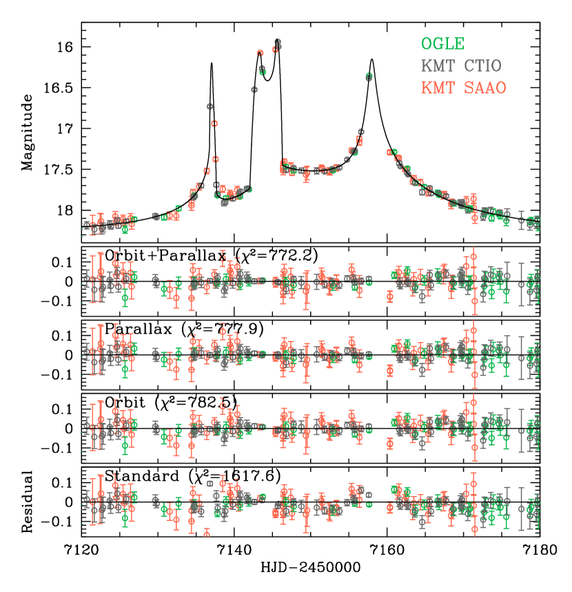
Figure 1.— Light curve of OGLE-2015-BLG-0768. Lower panels show residuals from various tested models and the $\chi^{2}$ values of the models. The curve superposed on the observed data is the best-fit model based on the “orbit+parallax” model.

2. Degeneracy: OGLE-2015-BLG-0768 Case

In order to describe a binary lensing light curves, one needs many parameters. A microlensing modeling is a process of finding a set of lensing parameters that results in the best-fit model light curve to the observed one. For the simplest case of a binary-lens event with a linear observer’s motion and a static binary, one needs 7 parameters and the number of parameters increases in order to consider higher-order effects like the microlens-parallax and lens-orbital effects. Furthermore, lensing parameters are usually tightly correlated one another (Han et al., 2010) and thus the parameters describing the microlens-parallax and lens-orbital effects are likely to be related not only to each other but also to other parameters. As a result, it is difficult to analytically track down the complex multi-dimensional correlations between parameters. We, therefore, show the severity of the degeneracy between the two higher-order effects for an example event where higher-order effects are needed to describe the observed light curve.

OGLE-2015-BLG-0768 is an exemplary lensing event where we find that the degeneracy between the microlens-parallax and lens-orbital effects is severe. The event occurred on a source star that is located toward the Galactic bulge field. The coordinates of the source are $({\rm RA},{\rm DEC})_{\rm J2000}=(17^{\rm h}38^{\rm m}19^{\rm s}\hskip-2.0pt.15,-27^{\circ}28^{\prime}02^{\prime\prime}\hskip-2.0pt.5)$, that correspond to the Galactic coordinates $(l,b)=(0.40^{\circ},2.14^{\circ})$. The lensing-induced brightening of the source star was discovered on 2015 April 22 by the Early Warning System (EWS) of the Optical Gravitational Lensing Experiment (OGLE) group that has conducted microlensing survey since 1992 using the 1.3m telescope located at the Las Campanas Observatory in Chile (Udalski et al., 1992). The event was also observed by the Korean Microlensing Telescope Network (KMTNet: Kim et al., 2016) survey that was commenced in 2015. The KMTNet survey is composed of three identical 1.6m telescopes that are located at Cerro Tololo Interamerican Observatory in Chile (KMT CTIO), South African Astronomical Observatory in South Africa (KMT SAAO), and Siding Spring Observatory in Australia (KMT SSO). The KMT CTIO and SAAO started their operation in February, 2015, but the KMT SSO was not yet operational at the time of the event. The KMTNet survey conducted with a $\sim 10$ minute cadence for its main field. The source star of the event was in the field that was observed with a $\sim 1/2$ – 1 day cadence mainly in support of the Spitzer microlensing program.

In Figure 1, we present the light curve of OGLE-2015-BLG-0768. It shows a complicated sequence of three peaks that occurred chronologically at ${\rm HJD}^{\prime}={\rm HJD}-2450000\sim 7137$, 7144, and 7158. The second peak is composed of two spikes where the region between them shows a “U”-shape trough. Such an anomaly is a characteristic feature that appears when a source crosses caustics, which represent the locations on the source plane at which a point-source magnification becomes infinity, formed by a binary lens, indicating that the event was occurred by a binary lens. The first and third peaks do not show such a caustic-crossing feature, suggesting that they were produced by either passing over or approaching tips of the caustic.

Considering the characteristic features of the light curve, we conduct binary-lens modeling of the light curve. We begin with a simplest case where the relative lens-source motion is linear. Among the 7 principal binary-lensing parameters for this standard modeling, 3 parameters describe the source-lens approach, including the time of the closest approach of the source to a reference position of the lens, $t_{0}$, the source-reference separation at that time, $u_{0}$, and the angle between the source trajectory and the binary axis, $\alpha$ (source trajectory angle). For the reference position in the lens plane, we use the center of mass of the binary lens. Another parameter $t_{\rm E}$ (Einstein time scale), which is defined as the time for the source to cross the angular Einstein radius $\theta_{\rm E}$ of the lens, represents the time scale of the event. The Einstein ring is the image of the source for the case of the exact lens-source alignment and it is used as a length scale in describing lensing phenomenon. Two other parameters characterize the binary lens including $s$ and $q$, which represent the projected separation and mass ratio, respectively. We note that the two parameters $u_{0}$ and $\alpha$ are normalized to $\theta_{\rm E}$. The last parameter $\rho$ is the ratio of the angular source radius $\theta_{*}$ to the angular Einstein radius, i.e. $\rho=\theta_{*}/\theta_{\rm E}$. This normalized source radius is needed to describe the caustic-crossing parts of the light curve that are affected by the finite size of the source star.

Table 1Lensing parameters

Parameters	Standard	Parallax	Orbit	Orbit+Parallax
$\chi^{2}$	1617.6	777.9	782.5	772.2
$t_{0}\ ({\rm HJD}-2450000)$	7156.157 $\pm$ 0.049	7154.669 $\pm$ 0.152	7155.099 $\pm$ 0.074	7154.931 $\pm$ 0.112
$u_{0}$	0.214 $\pm$ 0.001	0.253 $\pm$ 0.001	0.249 $\pm$ 0.001	0.248 $\pm$ 0.003
$t_{\rm E}\ ({\rm days})$	19.69 $\pm$ 0.04	20.35 $\pm$ 0.16	19.39 $\pm$ 0.06	20.08 $\pm$ 0.21
$s$	0.773 $\pm$ 0.001	0.778 $\pm$ 0.001	0.768 $\pm$ 0.002	0.763 $\pm$ 0.006
$q$	0.849 $\pm$ 0.019	0.791 $\pm$ 0.024	0.858 $\pm$ 0.018	0.798 $\pm$ 0.023
$\alpha\ ({\rm rad})$	1.179 $\pm$ 0.008	0.986 $\pm$ 0.015	1.023 $\pm$ 0.009	1.008 $\pm$ 0.011
$\rho\ (10^{-3})$	7.76 $\pm$ 0.23	8.40 $\pm$ 0.19	7.76 $\pm$ 0.23	8.08 $\pm$ 0.25
$\pi_{{\rm E},N}$	-	-4.52 $\pm$ 0.30	-	-2.26 $\pm$ 1.00
$\pi_{{\rm E},E}$	-	0.12 $\pm$ 0.25	-	-0.08 $\pm$ 0.22
$ds/dt$ $(yr^{-1})$	-	-	-0.23 $\pm$ 0.06	-0.46 $\pm$ 0.18
$d\alpha/dt$ $(yr^{-1})$	-	-	-2.55 $\pm$ 0.05	-0.89 $\pm$ 0.57

Modeling the light curve is proceeded in multiple steps. In the first step, we conduct a grid search in the space of the parameters $s$, $q$, and $\alpha$ for which lensing light curves vary sensitively to the changes of the parameters. We search for the other parameters by using a downhill approach based on the Markow Chain Monte Carlo (MCMC) method. In the second step, we identify local minima in the $\chi^{2}$ map of the parameters. We identify a unique minimum with a projected binary separation $s\sim 0.8$ and a mass ratio $q\sim 0.8$. In the next step, we gradually refine the identified minimum by allowing all parameters to vary.

We compute magnifications affected by the finite size of the source star using the combination of the numerical inverse-ray-shooting method (Schneider & Weiss, 1986) and the semi-analytic hexadecapole approximation (Pejcha & Heyrovský, 2009; Gould, 2008). In computing finite-source magnifications, we consider the surface-brightness variation of the source star caused by the limb-darkening effect by modeling the surface brightness profile as $S_{\lambda}\propto 1-\Gamma_{\lambda}(1-3\cos\psi/2)$, where $\psi$ is the angle between the line of sight toward the source center and the normal to the source surface and $\Gamma_{\lambda}$ is the linear limb-darkening coefficient. From the measurements of $I$ and $V$-band magnitudes of the source star followed by the calibration of the color and magnitudes using the centroid of giant clump in the color-magnitude diagram as a reference (Yoo et al., 2004), we find that the source star is a G-type giant with a de-reddened color and a magnitude $(V-I,I)_{0}=(0.86\pm 0.02,15.92\pm 0.01)$. Based on the source type, we adopt the limb-darkening coefficient of $\Gamma_{I}=0.49$.

In the bottom panel of Figure 1, we present the residual of the data from the best-fit “standard” model. It is found that data around the main features of the light curve exhibit noticeable deviations. Considering that the time gap between the first and last peaks, $\sim 20$ days, is considerable, the residual can be ascribed to higher-order effects. We, therefore, conduct additional modeling considering the higher-order effects. In the “parallax” and “orbit” models, we separately consider the microlens-parallax effect and lens-orbital effect, respectively. In the “orbit+parallax” model, we consider both effects.

Consideration of the microlens-parallax effect requires to include two additional parameters $\pi_{{\rm E},N}$ and $\pi_{{\rm E},E}$, which represent the two components of the microlens parallax vector $\mbox{\boldmath$\pi$}_{\rm E}$ projected onto the sky along the north and east equatorial coordinates, respectively. To first-order approximation, the lens-orbital effect is describe by two parameters $ds/dt$ and $d\alpha/dt$, which represent the change rates of the projected binary separation $s$ and the source trajectory angle $\alpha$, respectively. For the description of the full Keplerian orbital motion, one needs two more parameters $s_{\parallel}$ and $ds_{\parallel}/dt$, which are the line-of-sight separation between the binary components and its rate of change, respectively (Skowron et al., 2011). In our analysis, we consider the orbital effect with the two parameters $ds/dt$ and $d\alpha/dt$.

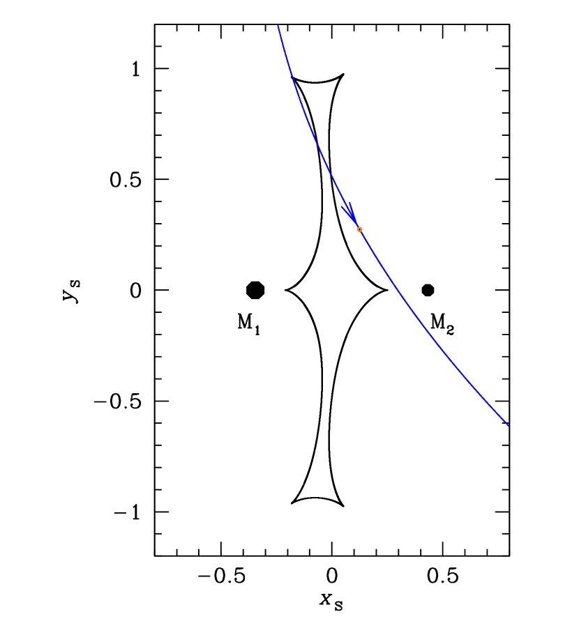
Figure 2.— Geometry of the lens system. The curve with an arrow represents the source trajectory with respect to the caustic which is the figure composed of concave curves. The Two filled dots marked by $M_{1}$ and $M_{2}$ ($<M_{1}$) are the locations of the binary lens components. Lengths are scaled to the Einstein radius corresponding to the total mass of the binary lens. The size of the tiny circle at the tip of the arrow on the source trajectory represents the source size. The model is based on the “orbit+parallax” model of which parameters are presented in Table 1. We note that the lens position and the resulting caustic vary in time due to the orbital motion of the lens and the presented positions are those at ${\rm HJD}=2457144$, which corresponds to the time of the second peak in the light curve presented in Fig. 1.

Table 2Degenerate solutions

Solution	$\chi^{2}$	$\pi_{{\rm E},N}$	$\pi_{{\rm E},E}$	$ds/dt$	$d\alpha/dt$
(1)	772.2	-2.26	-0.08	-0.46	-0.89
(2)	772.5	-3.32	0.00	-0.34	-0.39
(3)	772.6	-0.70	0.38	-0.54	-2.02
(4)	776.0	0.05	0.15	0.15	0.17

In Table 1, we summarize the results of modeling along with the $\chi^{2}$ values and the lensing parameters of the individual tested models. In the lower panels of Figure 1, we present the residuals of the models. The model light curve corresponding to the best-fit model, i.e. orbit+parallax, is plotted over the data in Figure 1. In Figure 2, we also present the geometry of the lens system showing the source trajectory with respect to the caustic for the best-fit model. Figure 2 shows that the event was produced by the passage of the source over a single large caustic formed by a resonant binary with a projected separation similar to the Einstein radius corresponding to the total mass of the binary, i.e. $s\sim 1$. The second peak was produced by the crossing of the source star over the caustic and first and third peaks were produced by the source star’s approaches to the tips of the caustic.

From the results of analysis, it is found that the fit greatly improves when higher-order effects are considered. We find that the consideration of the microlens-parallax effect improves the fit by $\Delta\chi^{2}=839.7$ with respect to the standard model. The consideration of the lens-orbital effect results in a similar fit improvement with $\Delta\chi^{2}=835.1$. However, the further improvement of the fit by considering both effects is meager: $\Delta\chi^{2}=5.7$ from the parallax model and $\Delta\chi^{2}=10.3$ from the orbital model. The fact that the $\chi^{2}$ improvements by the tested models are similar one another regardless of the considered higher-order effects strongly indicates that the lens-parallax and lens-orbital effects are difficult to be distinguished despite the obvious influence of the higher-order effects on the lensing light curve.

The degeneracy between the microlens-parallax and lens-orbital effects is also shown in Figure 3, where we plot the distribution of the parallax parameters $\pi_{{\rm E},N}$ and $\pi_{{\rm E},E}$ obtained from the orbit+parallax modeling. The color coding represents points on the MCMC chain within 1$\sigma$ (red), 2$\sigma$ (yellow), 3$\sigma$ (green), 4$\sigma$ (cyan), and 5$\sigma$ (blue) of the best fit value. One finds that the observed light curve is explained with parallax parameters that are distributed in a wide range of the parameter space. On the $\pi_{{\rm E},N}-\pi_{{\rm E},E}$ distribution plot, we mark 4 different solutions for which the parallax parameters and orbital parameters are presented in Table 2 along with the corresponding $\chi^{2}$ values. For the solution with a large $\pi_{\rm E}$ value, e.g. ‘Solution (2)’, the deviation from the standard model is explained mostly by the parallax effect. On the other hand, the solution with a small $\pi_{\rm E}$ value, e.g. ‘Solution (4)’, the deviation is mostly explained by the orbital effect. Despite the large difference between the parameters of the higher-order effects, $\chi^{2}$ differences among the solutions are very minor, indicating that the degeneracy between the microlens-parallax and lens-orbital effects are very severe.

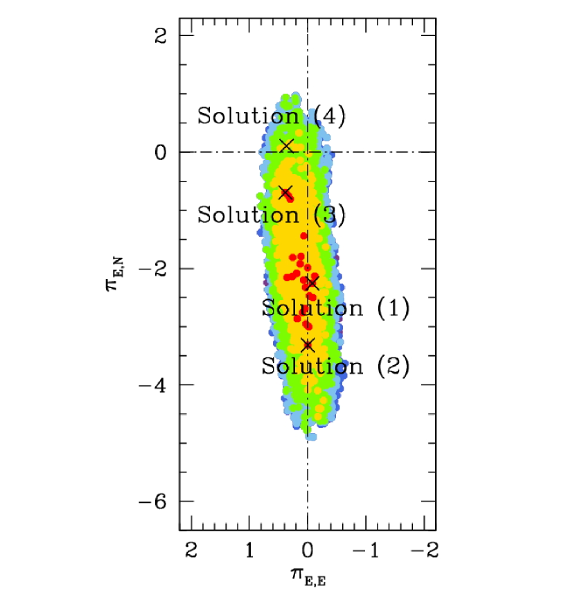
Figure 3.— Distribution of the parallax parameters $\pi_{{\rm E},N}$ and $\pi_{{\rm E},E}$. obtained from the orbit+parallax modeling. The color coding represents points on the MCMC chain within 1 (red), 2 (yellow), 3 (green), 4 (cyan), and 5 (blue) $\sigma$ of the best fit. The microlens-parallax parameters, $\pi_{{\rm E},N}$ and $\pi_{{\rm E},E}$, and the lens-orbital parameters, $ds/dt$ and $d\alpha/dt$, corresponding to the 4 solutions designated by (1) through (4) on the plot are presented in Table 2.

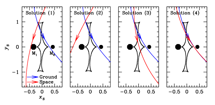
Figure 4.— Lens system geometry corresponding to the 4 solutions presented in Table 2. In each panel, the blue curve represents the source trajectory seen from the Earth and the red curve represents the source trajectory if the event were observed by the Spitzer telescope. Other notations are same as those in Fig. 2.

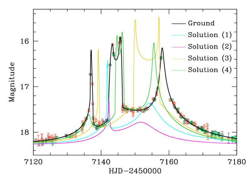
Figure 5.— Expected light curves from space-based observations using the Spitzer telescope for the 4 solutions in Table 2. Also presented is the best-fit model of the ground-based data.

3. Resolving the Degeneracy

In the previous section, we demonstrated that despite an obvious long-term deviation in a microlensing light curve it could be difficult to identify the cause of the deviation because of the difficulty in distinguishing between the microlens-parallax and lens-orbital effects. In this section, we show that the degeneracy can be readily resolved with the additional data provided by space-based microlens parallax observations.

Resolving the degeneracy with the space-based data will be possible because the degenerate solutions with different values of the microlens parallax will result in different lensing light curves when an event is observed by the satellite. We illustrate this for OGLE-2015-BLG-0768 that was used to show the severity of the degeneracy between the microlens-parallax and lens-orbital effects in the data obtained from ground-based observations. In Figure 4, we present the lens system geometry corresponding to the 4 solutions presented in Table 2. In each panel, the blue curve represents the source trajectory seen from the Earth and the red curve represents the source trajectory that is expected if the event were observed by the Spitzer telescope. As expected, one finds that the ground-based source trajectories of the individual solutions show similar paths with respect to the caustics, resulting in similar ground-based light curves. In contrast, the space-based trajectories have dramatically different paths from one another due to the differences in the values of the microlens parallax.

In Figure 5, we present the space-based light curves corresponding to the source trajectories that are marked in the individual panels of Figure 4. In order to show the level of difference between the ground-based and space-based light curves, we also present the ground-based data and the best-fit model. From the comparison of the light curves, it is found that despite the similarity in the ground-based light curves, the resulting space-based light curves of the individual solutions show dramatically different shapes. This indicates that the microlens parallax can be uniquely determined from the difference between the ground-based and space-based light curves and thus the severe degeneracy in the interpretation of the ground-based data can be readily resolved with the additional data provided by the space-based microlensing observations. Once the microlens parallax is determined, one can further constrain the orbital parameters of the lens by analyzing remaining residuals from the parallax model. Therefore, data from space-based microlens-parallax observations are important not only in accurately determining the basic lens parameters of the mass and distance but also in characterizing the orbital parameters of the lens.

The possibility of characterizing the orbital parameters of a binary lens was recently pointed out by Han et al. (2016), where they presented the analysis of the combined data from the ground-based and space-based Spitzer observations of the binary-lens event OGLE-2015-BLG-0479. Thanks to the uniquely determined microlens parallax with the space-based data, they were able to constrain the complete orbital parameters of the lens, although the uncertainties of the estimated orbital parameters are rather big due to the partial coverage of the event by the Spitzer data combined with the sparse coverage and modest photometry quality of the ground-based data. The precision will be improved with the expansion of both the ground-based and space-based surveys.

4. Conclusion

We demonstrated that interpretation of long-term deviations in lensing light curves could be difficult due to the severe degeneracy between the microlens-parallax and lens-orbital effects even for the case of obvious deviations. We also showed that the degeneracy could be readily resolved with the additional data from space-based microlens parallax observations. Being able to unambiguously determine the microlens parallax, space-based microlens observations will enable to determine the physical parameters of the lens with an increased accuracy. Furthermore, space-based data will make it possible to constrain the orbital parameters of the lens with an unprecedented precision.

References

- Bozza et al. (2016) Bozza, V., Shvartzvald, Y., Udalski, A., et al. 2016, ApJ, 820, 79
- Batista et al. (2011) Batista, V., Gould, A., Dieters, S., et al. 2011, A&A, 529, 102
- Calchi Novati et al. (2015) Calchi Novati, S., Gould, A., Udalski, A., et al. 2015, ApJ, 804, 20
- Dominik (1998) Dominik, M. 1998, A&A, 329, 361
- Gould (1992) Gould, A. 1992, ApJ, 392, 442
- Gould (1994) Gould, A. 1994, ApJ, 421, L75
- Gould (2000) Gould, A. 2000, ApJ, 542, 785
- Gould (2008) Gould, A. 2008, ApJ, 681, 1593
- Gould et al. (2014) Gould, A., Carey, S., & Yee, J. 2014, Spitzer Proposal ID#11006
- Han et al. (2010) Han, C., Hwang K.-H., & Ryu, Y.-H. 2010, ApJ, 720, 409
- Han et al. (2016) Han, C., Udalski, A., Gould, A., et al. 2016, ApJ, submitted
- Henderson et al. (2016) Henderson, C. B., Poleski, R., Penny, M., et al. 2016, ApJ, submitted
- Ioka et al. (1999) Ioka, K., Nishi, R., & Kan-Ya, Y. 1999, Prog. Theor. Phys., 102, 983
- Kim et al. (2016) Kim, S.-L., Lee, C.-U., Park, B.-G., et al. 2016, Journal of the Korean Astron. Soc., 49, 37
- Pejcha & Heyrovský (2009) Pejcha, O., & Heyrovský, D. 2009, ApJ, 690, 1772
- Refsdal (1966) Refsdal, S. 1966, MNRAS, 134, 315
- Schneider & Weiss (1986) Schneider, P., & Weiss, A. 1986, A&A, 164, 237
- Shvartzvald et al. (2015) Shvartzvald, Y., Udalski, A., Gould, A., et al. 2015, ApJ, 814, 111
- Skowron et al. (2011) Skowron, J., Udalski, A., Gould, A., et al. 2011, ApJ, 738, 87
- Street et al. (2016) Street, R. A. Udalski, A., Calchi Novati, A., et al. 2016, ApJ, 819, 93
- Shin et al. (2011) Shin, I.-G., Udalski, A., Han, C., et al. 2011, ApJ, 735, 85
- Udalski et al. (1992) Udalski, A. Szymański, M., Kalużny, J. Kubiak, M., & Mateo, M. 1992, Acta Astron., 42, 253
- Udalski et al. (2015) Udalski, A., Yee, J. C., Gould, A., et al. 2015b, ApJ, 799, 237
- Yee et al. (2015) Yee, J. C., Udalski, A.; Calchi Novati, S., et al. 2015, ApJ, 802, 76
- Yoo et al. (2004) Yoo, J., DePoy, D. L., Gal-Yam, A., et al. 2004, ApJ, 603, 139
- Zhu et al. (2015) Zhu, Wei, Udalski, A., Gould, A., et al. 2015, ApJ, 805, 8