Effect of strong $\bar{\rm p}$-p nuclear forces on the rate of the low-energy three-body protonium formation reaction: $\bar{\mbox{p}}+\mbox{H}_{\mu}(1s)\rightarrow(\bar{\mbox{p}}\mbox{p})_{\alpha}+\mu^{-}$

Abstract

The effect of the strong $\bar{\rm p}$-p nuclear interaction in a three-charge-particle system with arbitrary masses is investigated. Specifically, the ($\bar{\rm p},\ \mu^{-}$, p) system is considered, where $\bar{\mbox{p}}$ is an antiproton, $\mu^{-}$ is a muon and p is a proton. A numerical computation in the framework of a detailed few-body approach is carried out for the following protonium (antiprotonic hydrogen) formation three-body reaction: $\bar{\mbox{p}}+\mbox{H}_{\mu}(1s)\rightarrow(\bar{\mbox{p}}\mbox{p})_{\alpha}+\mu^{-}$. Here, $\mbox{H}_{\mu}(1s)$ is a ground state muonic hydrogen, i.e. a bound state of p and $\mu^{-}$. A bound state of p and its counterpart $\bar{\mbox{p}}$ is a protonium atom in a quantum atomic state $\alpha$, i.e. $Pn=(\bar{\mbox{p}}\mbox{p})_{\alpha}$. The low-energy cross sections and rates of the $Pn$ formation reaction are computed in the framework of a Faddeev-like equation. The strong $\bar{\rm p}$-p interaction is included in these calculations within a first order approximation. It was found, that even in the framework of this approximation the inclusion of the strong interaction results in a quite significant correction to the rate of the three-body reaction. Therefore, the title three-body antiprotonic process with participation of muons should be useful, especially at low-energy collisions, in studying the $\bar{\rm p}$-p nuclear forces and the annihilation channels in $Pn$.

I Introduction

The first detection and exploration of antiprotons, $\bar{\rm p}$’s, 1st_pbar occurred more than a half of a century ago. Since that time this research field, which is related to stable baryonic particles, has seen substantial developments in both experimental and theoretical aspects. This field of particle physics represents one of the most important sections of research work at CERN. It will suffice to mention such experimental research groups as ALPHA andresen10 , ATRAP gabr11 , ASACUSA hori2013 and others, which carry out experiments with antiprotons. By using slow antiprotons it is then possible to create ground state antihydrogen atoms $\bar{\mbox{H}}_{1s}$ (a bound state of $\bar{\mbox{p}}$ and $e^{+}$, i.e. a positron) at low temperatures. The resulting two-particle atom at present can be viewed as one of the simplest and most stable anti-matter species amoretti2002 . A comparison of the properties of the resulting hydrogen atom H with $\bar{\mbox{H}}$ reveals that this antiatom lends itself well to support testing of the fundamentals of physics nature2016 . For example, an evaluation of the CPT theorem comes to mind immediately vargas2015 . This possibility reinforces the need to obtain and store low-energy $\bar{\mbox{p}}$’s which could provide a basis for further comparisons of scientific interest. The system certainly contributes to the state of current research in both atomic and nuclear physics hori2013 ; madsen2015 ; gabr11 ; andresen10 . Further, the basic idea could be expanded to other atoms. A good example of this would be metastable antiprotonic helium atoms (atomcules) such as $\bar{\mbox{p}}^{3}$He⁺ and $\bar{\mbox{p}}^{4}$He⁺ hayano2007 . It is important to note that within the field of $\bar{\mbox{p}}$ physics these Coulomb three-body systems are also very important. Specifically, the use of high-precision laser spectroscopy of atomclues allows one to measure $\bar{\mbox{p}}$’s charge-to-mass ratio as well as fundamental constants within the standard model hori11 . Developments in regard to atomcules and $\bar{\mbox{H}}$ atoms have increased interest in the protonium ($Pn$) atom as well. This atom can be viewed as a bound state of $\bar{\mbox{p}}$ and p zurlo2006 ; venturelli07 ; rizzini2012 . The two-heavy-charge-particle system can also be described as antiprotonic hydrogen. Its characteristics within the atomic scale are that it is a heavy and an extremely small system containing strong Coulomb and nuclear interactions. There is an interplay between these interactions inside the atom. This situation is responsible for the creation of interesting resonance and quasi-bound states in $Pn$ shapiro1 . Thus, $Pn$ can be considered as a useful tool in the examination of the antinucleon$-$nucleon $(\bar{N}N)$ interaction potential np2015 ; jmr1992 ; jmr1982a ; jmr1982 as well as the annihilation processes desai1961 ; jmr2002 ; jmr2005 . In other words, the interplay between Coulomb and nuclear forces contributes greatly to $\bar{\mbox{p}}$ and p quantum dynamics shapiro2 . Further, the $\bar{\mbox{p}}+$p elastic scattering problem has also been examined in numerous papers. A good representative example would be paper jmr2002 . It is also worthwhile to note that $Pn$ formation is related to charmonium - a hydrogen-like atom $(\bar{c}c)$, which is also known as a bound state of a $c$-antiquark $(\bar{c})$ and $c$-quark jmr2002 . In sum, the fundamental importance of protonium and problems related to its formation, i.e. bound or quasi-bound states, resonances and spectroscopy, have resulted that this two-particle atom gained much attention in the last decades.

Several few-charge-particle collisions can be used in order to produce low-energy $Pn$ atoms. The following reaction is, for instance, one of them:

$$\bar{\mbox{p}}+\mbox{H}(1s)\rightarrow(\bar{\mbox{p}}\mbox{p})_{\alpha^{\prime}}+e^{-}.$$ (1)

This process is a Coulomb three-body collision which was computed in a few works in which different methods and techniques have been applied tong06 ; sakimoto13 ; esry03 . Because in this three-body process a heavy particle, i.e. a proton, is transferred from one negative ”center”, $e^{-}$, to another, $\bar{\mbox{p}}$, it would be difficult to apply a computational method based on an adiabatic (Born-Oppenheimer) approach born1927 . Besides, experimentalists use another few-body reaction to produce $Pn$ atoms, i.e. a collision between a slow $\bar{\mbox{p}}$ and a positively charged molecular hydrogen ion, i.e. H${}_{2}^{+}$: $\bar{\mbox{p}}+\mbox{H}_{2}^{+}\rightarrow(\bar{\mbox{p}}\mbox{p})_{\alpha^{\prime}}+\mbox{H}.$ Nonetheless, this paper is devoted to another three-body collision of the $Pn$ formation reaction in which we compute the cross-section and rate of a collision between $\bar{\mbox{p}}$ and a muonic hydrogen atom H_μ, which is a bound state of p and a negative muon:

$$\bar{\mbox{p}}+(\mbox{p}\mu)_{1s}\rightarrow(\bar{\mbox{p}}\mbox{p})_{\alpha}+\mu^{-},$$ (2)

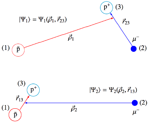
Figure 1: Two asymptotic spacial configurations of the three-body system (123), or more specifically $(\bar{\mbox{p}},\mu^{-},\rm{p}^{+})$, which are considered in this work. The few-body Jacobi coordinates $(\vec{\rho}_{i},\vec{r}_{jk})$, where $i\neq j\neq k=1,2,3$ are also shown together with the three-body wave function components $\Psi_{1}$ and $\Psi_{2}$: $\Psi=\Psi_{1}+\Psi_{2}$ is the total wave function of the three-body system.

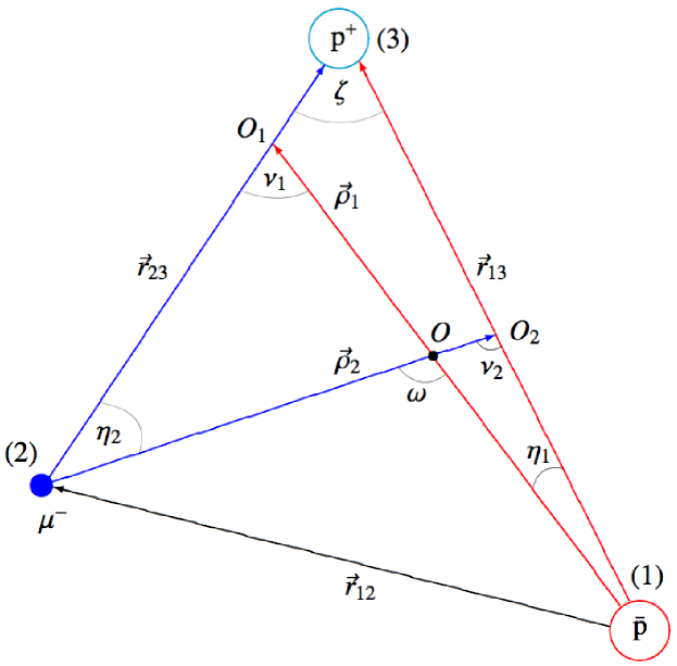
Figure 2: The title three-charge-particle system ${\bar{\rm p}},\mu^{-}$ and p⁺ (proton) and system’s configurational triangle $\triangle$123 are presented together with the few-body Jacobi coordinates (vectors): {$\vec{\rho}_{1},\vec{r}_{23}$} and {$\vec{\rho}_{2},\vec{r}_{13}$}. Additionally, $\vec{r}_{12}$ is the vector between two negative particles in the system. The necessary geometrical angles between the vectors such as $\eta_{1(2)},\nu_{1(2)},\zeta$ and $\omega$ are also shown in this figure.

where, $\alpha$=$1s$, $2s$ or $2p$ is the final quantum atomic state of $Pn$. Since the participation of $\mu^{-}$ in (2), at low-energy collisions $Pn$ would be formed in a very small size - in the ground and close to ground states $\alpha$. It is obvious that in these states the hadronic nuclear force between $\bar{\mbox{p}}$ and p will be strong and pronounced. In its ground state the $Pn$ atom has the following size: $a_{0}(Pn)=\hbar^{2}/(e_{0}^{2}m_{p}/2)\sim$ 50 fm, in which the Coulomb interaction between $\bar{\mbox{p}}$ and p becomes extremely strong. The corresponding $Pn$’s binding energy without the inclusion of the nuclear $\bar{\rm p}$-p interaction is: $E_{n}(Pn)=-e_{0}^{4}m_{p}/2/(2\hbar n^{2})\sim-$ 10 keV. We take: $n=1$, $\hbar$ is the Planck constant, $e_{0}$ is the electron charge, and $m_{p}$ is the proton mass. It would be useful to note, that the realistic $\bar{\rm p}$-p binding energy (with the inclusion of the strong nuclear interaction) can have a large value. This value may be comparable or even larger than $m_{p}$. Consequently, it might be necessary to apply a relativistic treatment to the reaction (2) in the output channel ueda . The situation which involves a very strong Coulomb interaction inside $Pn$ can also be a reason for vacuum polarization forces as well. Therefore, within the reaction (2) it might be quite useful to take into account all these physics effects and carry out a computation of their influence on the reaction’s partial cross sections and rates. Moreover, if in the near future it would be possible to undertake a high quality measurement of (2), we could compare the new results with corresponding theoretical data and fit (adjust) the $\bar{\rm p}$-p strong interaction into the theoretical calculation in order to reproduce the laboratory data. This process will be useful in order to better understand the annihilation processes and the nature of the strong $\bar{\rm p}$-p interaction. Muons are already used as an effective tool to search for ”new physics” and to carry out precise measurements of some fundamental constants lauss2009 . For example, in the atomic analog of the reaction (2) $Pn$ would be formed at highly excited Rydberg states with $\alpha^{\prime}\approx 30$. Therefore, it is interesting to investigate the $\bar{\rm p}$-p nuclear interaction in the framework of the three-body reaction (2) at low-energy collisions. In this paper the reaction (2) is treated as a Coulomb three-body system (123) with arbitrary masses: $m_{1},\ m_{2}$, and $m_{3}$. This is shown in Figs. 1 and 2. A few-body method based on a Faddeev-type equation formalism is used. In this approach the three-body wave function is decomposed in two independent Faddeev-type components fadd ; fadd93 . Each component is determined by its own independent Jacobi coordinates. Since, the reaction (2) is considered at low energies, i.e. well below the three-body break-up threshold, the Faddeev-type components are quadratically integrable over the internal target variables $\vec{r}_{23}$ and $\vec{r}_{13}$. They are also shown in Fig. 1. In this work the nuclear $\bar{\rm p}$-p interaction is included approximately by shifting the Coulomb (atomic) energy levels in $Pn$. In the next sections we will introduce notations pertinent to the few-body system (123), the basic equations, boundary conditions, and a brief derivation of the set of coupled one-dimensional integral-differential equations. The muonic atomic units (m.a.u. or m.u.) are used in this work: $e=\hbar=m_{\mu}=1$, $m_{\mu}=206.769\ m_{e}$ is the mass of the muon, $m_{e}$ is the electron mass, the proton (anti-proton) mass is $m_{p}=m_{\bar{p}}$=1836.152 $m_{e}$.

II A few-body approach

The main thurst of this paper is the three-body reaction (2). As we have already mentioned, a quantum-mechanical Faddeev-type few-body method is applied in this work. A coordinate space representation is used. In general, the Faddeev approach is based on a reduction of the total three-body wave function $\Psi$ on three Faddeev-type components fadd93 . However, when one has two negative and one positive charges only two asymptotic configurations are possible below the system’s total energy $(E)$ break-up threshold. This situation is explained in Fig. 1 specifically for the case of the three-body system: $\bar{\mbox{p}},\ \mu^{-}$ and $\mbox{p}^{+}$. In the framework of an adiabatic hyperspherical close-coupling approach the Coulomb three-body system has been considered in Ref. igarashi2008 . Nevertheless, one can also apply a few-body type method to the three-body system in which one can decompose $\Psi$ on two components and devise a set of two coupled equations hahn72 . Additionally, it would be interesting to investigate and estimate the effect of the strong $\bar{\rm p}$-p nuclear interaction in the final state of the reaction (2). This is done in the current work. For a number of reasons the direct $\bar{\rm p}$-p annihilation channel in (2) is not included in the current calculations. This approximation is discussed at the end of the following subsection.

II.1 Coupled integral-differential equations

A modified close coupling approach (MCCA) is applied in this work in order to solve the Faddeev-Hahn-type (FH-type) equations my2000 ; my2013 ; my03 . In other words, we carry out an expansion of the Faddeev-type components into eigenfunctions of the subsystem Hamiltonians. This technique provides an infinite set of coupled one-dimensional integral-differential equations. Within this formalism the asymptotic of the full three-body wave function contains two parts corresponding to two open channels merkur . One can use the following system of units: $e=\hbar=m_{2}=1$. We denote an antiproton $\bar{\rm{p}}$ by 1, a negative muon $\mu^{-}$ by 2, and a proton p by 3. The total Hamiltonian of the three-body system is:

$$\hat{H}=\hat{H}_{0}+V_{12}(\vec{r}_{12})+V_{23}(\vec{r}_{23})+\mathbb{V}_{13}(\vec{r}_{13}),$$ (3)

where $\hat{H}_{0}$ is the total kinetic energy operator of the three-body system, $V_{12}(\vec{r}_{12})$ and $V_{23}(\vec{r}_{23})$ are Coulomb pair-interaction potentials between particles 12 and 23 respectively, and:

$$\mathbb{V}_{13}(\vec{r}_{13})=V_{13}(\vec{r}_{13})+v_{13}^{\bar{N}N}(\vec{r}_{13})$$ (4)

is the Coulomb+nuclear interaction between particles 13, i.e. $\bar{\rm{p}}$ and p. $v_{13}^{\bar{N}N}(\vec{r}_{13})$ is the $\bar{N}N$ strong short-range interaction between the particles. The last potential is considered as an approximate spherical symmetric intgeraction in this work. The system is depicted in Figs. 1 and 2 together with the Jacobi coordinates $\{\vec{r}_{j3},\vec{\rho}_{k}\}$ and the different geometrical angles between the vectors:

$$\vec{r}_{j3}=\vec{r}_{3}-\vec{r}_{j},$$ (5)

$$\vec{\rho}_{k}=\frac{(m_{3}\vec{r}_{3}+m_{j}\vec{r}_{j})}{(m_{3}+m_{j})}-\vec{r}_{k},\ \ \ (j\not=k=1,2).$$ (6)

Here $\vec{r}_{\xi}$, $m_{\xi}$ are the coordinates and the masses of the particles $\xi=1,2,3$ respectively. This circumstance suggests a few-body Faddeev formulation which uses only two components. A general procedure to derive such formulations is described in Ref. hahn72 . In this approach the three-body wave function is represented as follows:

$$|\Psi\rangle=\Psi_{1}(\vec{r}_{23},\vec{\rho}_{1})+\Psi_{2}(\vec{r}_{13},\vec{\rho}_{2}),$$ (7)

where each Faddeev-type component is determined by its own Jacobi coordinates. Moreover, $\Psi_{1}(\vec{r}_{23},\vec{\rho}_{1})$ is quadratically integrable over the variable $\vec{r}_{23}$, and $\Psi_{2}(\vec{r}_{13},\vec{\rho}_{2})$ over the variable $\vec{r}_{13}$. To define $|\Psi_{l}\rangle$, $(l=1,2)$ a set of two coupled Faddeev-Hahn-type equations would be:

$$\Big{(}E-\hat{H}_{0}-V_{23}(\vec{r}_{23})\Big{)}\Psi_{1}(\vec{r}_{23},\vec{\rho}_{1})=\Big{(}V_{23}(\vec{r}_{23})+V_{12}(\vec{r}_{12})\Big{)}\Psi_{2}(\vec{r}_{13},\vec{\rho}_{2}),$$ (8)

$$\Big{(}E-\hat{H}_{0}-\mathbb{V}_{13}(\vec{r}_{13})\Big{)}\Psi_{2}(\vec{r}_{13},\vec{\rho}_{2})=\Big{(}\mathbb{V}_{13}(\vec{r}_{13})+V_{12}(\vec{r}_{12})\Big{)}\Psi_{1}(\vec{r}_{23},\vec{\rho}_{1}).$$ (9)

Here, $\hat{H}_{0}$ is the kinetic energy operator of the three-particle system, $V_{ij}(r_{ij})$ are paired Coulomb interaction potentials $(i\not=j=1,2,3)$, $E$ is the total energy, and $\mathbb{V}_{13}(\vec{r}_{13})$ is represented in Eq. (4). It is important to point out here, that the constructed equations satisfy the Schrődinger equation exactly hahn72 . For the energies below the three-body break-up threshold these equations exhibit the same advantages as the Faddeev equations fadd , because they are formulated for the wave function components with correct physical asymptotes.

Next, the kinetic energy operator $\hat{H}_{0}$ in Eqs. (8)-(9) can be represented as: $\hat{H}_{0}=\hat{T}_{\rho_{i}}+\hat{T}_{r_{ij}}$, then one can re-write the equations (8)-(9) in the following way:

$$\Big{(}E-\hat{T}_{\rho_{1}}-\hat{h}_{23}(\vec{r}_{23})\Big{)}\Psi_{1}(\vec{r}_{23},\vec{\rho}_{1})=\Big{(}V_{23}(\vec{r}_{23})+V_{12}(\vec{r}_{12})\Big{)}\Psi_{2}(\vec{r}_{13},\vec{\rho}_{2}),$$ (10)

$$\Big{(}E-\hat{T}_{\rho_{2}}-\hat{h}^{\bar{N}N}_{13}(\vec{r}_{13})\Big{)}\Psi_{2}(\vec{r}_{13},\vec{\rho}_{2})=\Big{(}V_{13}(\vec{r}_{13})+v^{\bar{N}N}_{13}(\vec{r}_{13})+V_{12}(\vec{r}_{12})\Big{)}\Psi_{1}(\vec{r}_{23},\vec{\rho}_{1}).$$ (11)

The two-body target hamiltonians $\hat{h}_{23}(\vec{r}_{23})=\hat{T}_{\vec{r}_{23}}+V_{23}(\vec{r}_{23})$ and $\hat{h}^{\bar{N}N}_{13}(\vec{r}_{13})=\hat{T}_{\vec{r}_{13}}+V_{13}(\vec{r}_{13})+v^{\bar{N}N}_{13}(\vec{r}_{13})$ with an additional $\bar{\rm p}$-p nuclear interaction are represented explicitly in these equations. In order to solve Eqs. (10)-(11) a modified close-coupling approach is applied, which leads to an expansion of the system’s wave function components $\Psi_{1}$ and $\Psi_{2}$ into eigenfunctions $\varphi^{(1)}_{n}(\vec{r}_{23})$ and $\varphi^{(2)\bar{N}N}_{n^{\prime}}(\vec{r}_{13})$ of the subsystem (target) Hamiltonians, i.e.

$$\left\{\begin{array}[]{l}\Psi_{1}(\vec{r}_{23},\vec{\rho}_{1})\approx\ \ \ {\large{{\mathclap{\displaystyle\int}\mathclap{\sum_{n}}}}}\hskip 11.38109ptf^{(1)}_{n}(\vec{\rho}_{1})\varphi^{(1)}_{n}(\vec{r}_{23}),\\ \Psi_{2}(\vec{r}_{13},\vec{\rho}_{2})\approx\ \ \ {\large{{\mathclap{\displaystyle\int}\mathclap{\sum_{n^{\prime}}}}}}\hskip 11.38109ptf^{(2)}_{n^{\prime}}(\vec{\rho}_{2})\varphi^{(2)\bar{N}N}_{n^{\prime}}(\vec{r}_{13}).\end{array}\right.$$ (14)

This provides a set of coupled one-dimensional integral-differential equations after the partial-wave projection.

The two complete sets of functions, i.e. $\{\varphi_{n}^{(1)}(\vec{r}_{23})\}$ and $\{\varphi_{n^{\prime}}^{(2)\bar{N}N}(\vec{r}_{13})\}$, represent the eigenfunctions of the two-body target hamiltonians $\hat{h}_{23}(\vec{r}_{23})$ and $\hat{h}^{\bar{N}N}_{13}(\vec{r}_{13})$ respectively:

$$\hat{h}_{23}(\vec{r}_{23})\varphi_{n}^{(1)}(\vec{r}_{23})=\Big{[}\hat{T}_{\vec{r}_{23}}+V_{23}(\vec{r}_{23})\Big{]}\varphi_{n}^{(1)}(\vec{r}_{23})=\varepsilon_{n}\varphi_{n}^{(1)}(\vec{r}_{23})$$ (15)

$$\hat{h}^{\bar{N}N}_{13}(\vec{r}_{13})\varphi^{(2)\bar{N}N}_{n^{\prime}}(\vec{r}_{13})=\Big{[}\hat{T}_{\vec{r}_{13}}+V_{13}(\vec{r}_{13})+v^{\bar{N}N}_{13}(\vec{r}_{13})\Big{]}\varphi^{(2)\bar{N}N}_{n^{\prime}}(\vec{r}_{13})=\mathcal{E}_{n^{\prime}}\varphi^{(2)\bar{N}N}_{n^{\prime}}(\vec{r}_{13})$$ (16)

In addition to the Coulomb potential, the strong interaction, $v^{\bar{N}N}_{13}(\vec{r}_{13})$, is also included in Eq. (16). Coulomb is a central symmetric potential. Therefore, the eigenfunctions $\varphi_{n}^{(1)}$ and the corresponding eigenstates are landau :

$$\varphi_{n}^{(1)}(\vec{r}_{23})=\sum_{lm}R^{(1)}_{nl}(r_{23})Y_{lm}(\vec{r}_{23}),$$ (17)

$$\varepsilon_{n}=-\frac{\mu_{1}}{2n^{2}}.$$ (18)

The full potential between $\bar{\rm p}$ and p is more complex, because its second part, $v^{\bar{N}N}_{13}(\vec{r}_{13})$, posses an asymmetric $\bar{N}N$ nuclear interaction jmr2002 ; jmr2005 . We did not explicitly include the strong interaction in the current calculations. Therefore, in the case of the target $Pn$ eigenfunctions we used the two-body pure Coulomb (atomic) wave functions. Nonetheless, the strong $\bar{\rm p}$-p interaction is approximately taken into account in this work through the eigenstates $\mathcal{E}_{n^{\prime}}$ which have shifted values from the original Coulomb levels $\varepsilon_{n^{\prime}}$ deser , that is:

$$\varphi^{(2)\bar{N}N}_{n^{\prime}}(\vec{r}_{13})\approx\sum_{l^{\prime}m^{\prime}}R^{(2)\bar{N}N}_{n^{\prime}l^{\prime}}(r_{13})Y_{l^{\prime}m^{\prime}}(\vec{r}_{13})\approx\sum_{l^{\prime}m^{\prime}}R^{(2)}_{n^{\prime}l^{\prime}}(r_{13})Y_{l^{\prime}m^{\prime}}(\vec{r}_{13})$$ (19)

$$\mathcal{E}_{n^{\prime}}\approx\varepsilon_{n^{\prime}}+\Delta E_{n^{\prime}}^{\bar{N}N}=-\frac{\mu_{2}}{2n^{\prime 2}}+\Delta E_{n^{\prime}}^{\bar{N}N}.$$ (20)

In Eqs. (17) and (19) $Y_{lm}(\vec{r})$ are spherical functions varshal and $R^{(i)}_{nl}(r)$ $(i=1,2)$ is an analytical solution to the radial part of the two-charge-particle Schrődinger equation landau :

$$\Big{(}\varepsilon_{n}^{(i)}+\frac{1}{2\mu_{j}r_{j3}^{2}}\Big{\{}\frac{\partial}{\partial r_{j3}}\Big{(}r_{j3}^{2}\frac{\partial}{\partial r_{j3}}\Big{)}-l(l+1)\Big{\}}-V_{j3}\Big{)}R_{nl}^{(i)}(r_{j3})=0,$$ (21)

where $j\neq i=1,2$. The method outlined above is only a first order approximation. In the framework of this approach it would be interesting to estimate the level of influence of the strong $\bar{\rm{p}}-$p interaction on the three-charge-particle proton transfer reaction (2).

Broadly speaking, the two-body Coulomb-nuclear wave functions of $Pn$, i.e. $\varphi^{(2)\bar{N}N}_{n^{\prime}}(\vec{r}_{13})$ and corresponding eigenstates, $\mathcal{E}_{n^{\prime}}$, have been of a significant interest for a long time. To build these states one needs to solve the two-charge-particle Schrődinger equation with an additional strong short-range $\bar{N}N$ interaction, i.e. Eq. (16), see for instance jmr1982 . In Ref. armour2005 the authors explicitly included the nuclear $\bar{\rm{p}}$-p interaction in the framework of a variational approach for the case of the $\bar{\rm{H}}$+H scattering. However, as a first step, one can also apply an approximate approach: Eqs. (17)-(19) with an energy shift in the eigenstate of $Pn$ $\mathcal{E}_{n^{\prime}}$, i.e. Eq. (20), $\varepsilon_{n^{\prime}}$ is the Coulomb level and $\Delta E_{n^{\prime}}^{\bar{N}N}$ is its nuclear shift. It can be computed, for example, with the use of the following formula deser :

$$\Delta E^{\bar{N}N}_{n^{\prime}}=-\frac{4}{n^{\prime}}\frac{a_{s}}{B_{Pn}}\varepsilon_{n^{\prime}},$$ (22)

where $a_{s}$ is the strong interaction scattering length in the $\bar{\mbox{p}}+$p collision, i.e. without inclusion of the Coulomb interaction between the particles, $B_{Pn}$ is the Bohr radius of $Pn$. In the literature one can find other approximate expressions to compute $\Delta E^{\bar{N}N}_{n^{\prime}}$, see for example trueman ; popov1979 . It would also be interesting to apply some of these formulas in conjunction with the relativistic effects in protonium, see for example works ueda ; thaler1983 .

After determining a proper angular momentum expansion one can obtain an infinite set of coupled integral-differential equations for the unknown functions $f_{\alpha}^{(1)}(\rho_{1})$ and $f_{\alpha^{\prime}}^{(2)}(\rho_{2})$ my2013 :

$$\left\{\begin{aligned} \left[(k^{(1)}_{n})^{2}\ +\ \frac{\partial^{2}}{\partial\rho_{1}^{2}}\ -\ \frac{\lambda(\lambda+1)}{\rho_{1}^{2}}\right]f_{\alpha}^{(1)}(\rho_{1})=g_{1}\sum_{\alpha^{\prime}}\frac{\sqrt{(2\lambda+1)(2\lambda^{\prime}+1)}}{2L+1}\\ \times\int_{0}^{\infty}d\rho_{2}f_{\alpha^{\prime}}^{(2)}(\rho_{2})\int_{0}^{\pi}d\omega\sin\omega R_{nl}^{(1)}(|\vec{r}_{23}|)\left[-\frac{1}{|\vec{r}_{23}|}+\frac{1}{|\vec{r}_{12}|}\right]R_{n^{\prime}l^{\prime}}^{(2)}(|\vec{r}_{13}|)\\ \times\rho_{1}\rho_{2}\sum_{mm^{\prime}}D_{mm^{\prime}}^{L}(0,\omega,0)C_{\lambda 0lm}^{Lm}C_{\lambda^{\prime}0l^{\prime}m^{\prime}}^{Lm^{\prime}}Y_{lm}(\nu_{1},\pi)Y^{*}_{l^{\prime}m^{\prime}}(\nu_{2},\pi),\\ \\ \left[(k^{(2)}_{n})^{2}\ +\ \frac{\partial^{2}}{\partial\rho_{2}^{2}}\ -\ \frac{\lambda^{\prime}(\lambda^{\prime}+1)}{\rho_{2}^{2}}\right]f_{\alpha}^{(2)}(\rho_{2})=g_{2}\sum_{\alpha^{\prime}}\frac{\sqrt{(2\lambda+1)(2\lambda^{\prime}+1)}}{2L+1}\\ \times\int_{0}^{\infty}d\rho_{1}f_{\alpha^{\prime}}^{(1)}(\rho_{1})\int_{0}^{\pi}d\omega\sin\omega R_{nl}^{(2)}(|\vec{r}_{13}|)\left[-\frac{1}{|\vec{r}_{13}|}+\frac{1}{|\vec{r}_{12}|}\right]R_{n^{\prime}l^{\prime}}^{(1)}(|\vec{r}_{23}|)\\ \times\rho_{2}\rho_{1}\sum_{mm^{\prime}}D_{mm^{\prime}}^{L}(0,\omega,0)C_{\lambda 0lm}^{Lm}C_{\lambda^{\prime}0l^{\prime}m^{\prime}}^{Lm^{\prime}}Y_{lm}(\nu_{2},\pi)Y^{*}_{l^{\prime}m^{\prime}}(\nu_{1},\pi).\end{aligned}\right.$$ (23)

Here: $g_{i}=4\pi M_{i}/\gamma^{3}$ $(i=1,2)$, $L$ is the total angular momentum of the three-body system, $\alpha=(nl\lambda)$ are quantum numbers of a three-body state, $k_{n}^{(i)}=\sqrt{2M_{i}(E-E_{n}^{(j)})}$, with $M_{1}=(m_{2}+m_{3})m_{1}/(m_{1}+m_{2}+m_{3})$, $M_{2}=(m_{1}+m_{3})m_{2}/(m_{1}+m_{2}+m_{3})$, $E_{n}^{(j)}$ is the binding energy of $(j3)$, $(i\neq j=1,2)$, $\gamma=1-m_{1}m_{2}/((m_{1}+m_{3})(m_{2}+m_{3}))$, $D_{mm^{\prime}}^{L}(0,\omega,0)$ is the Wigner function varshal , $C_{\lambda 0lm}^{Lm}$ is the Clebsh-Gordon coefficient varshal , $\omega$ is the angle between the Jacobi coordinates $\vec{\rho}_{i}$ and $\vec{\rho}_{i^{\prime}}$, $\nu_{i}$ is the angle between $\vec{r}_{i^{\prime}3}$ and $\vec{\rho}_{i}$, $\nu_{i^{\prime}}$ is the angle between $\vec{r}_{i3}$ and $\vec{\rho}_{i^{\prime}}$. The following relationships should be used for the numerical calculations:

$$\sin\nu_{i}=\frac{\rho_{i^{\prime}}}{\gamma r_{i^{\prime}3}}\sin\omega,$$ (24)

$$\cos\nu_{i}=\frac{1}{\gamma r_{i^{\prime}3}}(\beta_{i}\rho_{i}+\rho_{i^{\prime}}\cos\omega),\ \ \ (i\neq i^{\prime}=1,2).$$ (25)

A detailed few-body treatment of the heavy-charge-particle reaction (2) is the main goal of this work. The geometric angles of the configurational triangle $\triangle$123: $\nu_{1(2)}$, $\eta_{1(2)}$, $\zeta$, and $\omega$ are shown in Fig. 2 together with the Jacobi coordinates, i.e. $\{\vec{r}_{j3},\ \vec{\rho}_{k}\}$ $(j\neq k=1,2)$ and $\vec{r}_{12}$. The center of mass of the (123) system is $O$. $O_{1}$ and $O_{2}$ are the center of masses of the targets. The Faddeev decomposition avoids over-completeness problems because the subsystems are treated in an equivalent way in the framework of the two-coupled equations. Thus, the correct asymptotes are guaranteed. The Faddeev-components are smoother functions of the coordinates than the total wave function fadd93 ; merkur .

In the framework of the first order approximation approach the direct $\bar{\rm p}$-p annihilation channel in the reaction (2) is not included in this work. In the input channel of the reaction (2), $\bar{\mbox{p}}$+(p${}^{+}\mu^{-})_{1s}$, the relatively heavy muon very effectively screens the strong Coulomb potential of the proton, and therefore it significantly prevents direct annihilation in (2) before the $Pn$ formation. In other words, the $Pn$ formation process dominates. However, it is another matter in the case of the atomic version of the $Pn$ formation reaction (1). Here, the electron cloud around the proton can also block the $\bar{\mbox{p}}$ movement to p, but because of the quantum-tunneling effect the massive antiproton can penetrate with a significant probability through the light electron cloud and then directly annihilate with proton before protonium forms. Therefore, in the framework of the reaction (1) it would be necessary to take into account the tunneling effect. As far as we know, this is still not done in a suitable way.

In terms of the $Pn$ annihilation in the reaction (2) (which can occur after the two-body system formation) and an inclusion of this effect in calculations, it was mentioned above that in this case one needs to build precise Coulomb-nuclear $\bar{\rm p}$-p two-body wave functions $\varphi^{(2)\bar{N}N}_{n^{\prime}}(\vec{r}_{13})$ from Eq. (16). In this special case, one needs to consider not only the shifts of the Coulomb levels Eqs. (20), but also their widths. However, in the current work, as a first order approximation the nuclear effect is considered only through Eqs. (20) and (22).

We believe that to some extent this approximation is justified. In this work, we were mostly interested in the $Pn$ atom formation process (2), where the values of the Coulomb-nuclear atomic levels at which the atom can form are important. As we mentioned, these levels have widths, but they are mostly responsible for the annihilation reaction that follows.

II.2 Boundary conditions

To reach the next step it is necessary to obtain a unique solution for equations (23). While doing so it is important that the appropriate boundary conditions are chosen. They should be related to the physical situation of the system. The following condition is imposed first:

$$f_{nl}^{(i)}(0)\mathop{\mbox{\large$\sim$}}0.$$ (26)

Subsequently, it is then appropriate to solve the three-body charge-transfer problem to utilize the ${\bf K}-$matrix formalism approach. This would appear to be a prudent step because this method has been successfully used to obtain solutions in various three-body problems within the framework of both the Schrődinger equation melezhik ; cohen91 and the coordinate space Faddeev equation kvits1995 . Specifically, in regard to the rearrangement scattering problem $i+(j3)$ as the initial state within the asymptotic region it will be necessary to devise two solutions to Eqs. (23) which then will satisfy the boundary conditions that follow:

$$\left\{\begin{array}[]{l}f_{1s}^{(i)}(\rho_{i})\mathop{\mbox{\large$\sim$}}\limits_{\rho_{i}\rightarrow+\infty}\sin(k^{(i)}_{1}\rho_{i})+K_{ii}\cos(k^{(i)}_{1}\rho_{i})\vspace{1mm}\\ f_{1s}^{(j)}(\rho_{j})\mathop{\mbox{\large$\sim$}}\limits_{\rho_{j}\rightarrow+\infty}\sqrt{v_{i}/v_{j}}K_{ij}\cos(k^{(j)}_{1}\rho_{j})\;,\\ \end{array}\right.$$ (29)

where $\it K_{ij}$ represents the appropriate scattering coefficients, and $v_{i(j)}$ ($i\neq j=1,2$) is the $i(j)$ channel velocity between the particles. Next, one can use the following change of variables in Eq. (23), i.e.

$${\sf f}_{1s}^{(i)}(\rho_{i})=f_{1s}^{(i)}(\rho_{i})-\sin(k^{(i)}_{1}\rho_{i}),\ \ \ (i=1,2).$$ (30)

This substitution results in a modification of the variables and provides two sets of inhomogeneous equations which can now be conveniently solved numerically. Some details of our numerical approach are presented below (See Appendix).The transition also allows the coefficients $K_{ij}$ to be gained by reaching a numerical solution for the previously described FH-type equations. Now the cross section can be expressed as follows:

$$\sigma_{ij}=\frac{4\pi}{k_{1}^{(i)2}}\left|\frac{{\bf K}}{1-i{\bf K}}\right|^{2}=\frac{4\pi}{k_{1}^{(i)2}}\frac{\delta_{ij}D^{2}+{\it K}_{ij}^{2}}{(D-1)^{2}+({\it K}_{11}+{\it K}_{22})^{2}}\ ,$$ (31)

where ($i,j=1,2$) refer to the two channels and $D=K_{11}K_{22}-K_{12}K_{21}$. Next, in accord with the quantum-mechanical unitarity principle the scattering matrix $\bf K=\begin{pmatrix}K_{11}&K_{12}\\ K_{21}&K_{22}\end{pmatrix}$ has an important feature, i.e. $K_{12}=K_{21}$, or:

$$\chi(E)=\frac{K_{12}}{K_{21}}=1.$$ (32)

The last equation has been checked for all considered collision energies within the framework of the 1s, 1s+2s and 1s+2s+2p MCCA approximations, i.e. Eqs. (14).

III Results

In this section we present our results. The $Pn$ formation three-body reaction is computed at low energies. A Faddeev-like equation formalism Eqs. (10)-(11) has been applied. The few-body approach has been explained in previous sections. In order to solve the coupled equations two different independent sets of target expansion functions have been employed (14). In the framework of this approach the two targets are treated equivalently and the method allows us to avoid the over-completeness problem. The goal of this paper is to carry out a reliable quantum-mechanical computation of the cross sections and corresponding rates of the $Pn$ formation reaction at low and very low collision energies. It is very interesting to estimate the influence of the strong short-range $\bar{\rm p}$-p interaction on the rate of the reaction (2). The three-body reaction (2) could be used to investigate the strong $\bar{\rm p}$-p nuclear interaction and the annihilation process in future experiments with the anti-protonic hydrogen atom or protonium $Pn$. The coupled integral-differential Eqs. (23) have been solved numerically for the case of the total angular momentum $L=0$ in the framework of the two-level 2$\times$(1s), four-level 2$\times$(1s+2s), and six-level 2$\times$(1s+2s+2p) close coupling approximations in Eq. (14). The sign ”2$\times$” indicates that two different sets of expansion functions are applied. The $L=0$ computation is justified, because we are interested in a very low-energy collision: $\varepsilon_{coll}\sim 10^{-4}$ eV$-$10 eV. The following boundary conditions (26), (29), and (30) have been applied. To compute the charge transfer cross sections the expression (31) has been used.

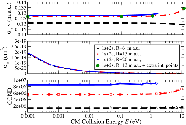
Figure 3: Upper plot: numerical convergence results for the low-energy proton transfer reaction integral cross section $\sigma_{tr}$ multiplied by the collision velocity v $=v_{c.m.}$, i.e. $\sigma_{tr}$v, in the three-body reaction $\bar{\rm{p}}+\rm{H}_{\mu}\rightarrow(\bar{\rm{p}}\rm{p})_{\alpha}+\mu^{-}$. Here, $\rm{H}_{\mu}$ is a muonic hydrogen atom and $\alpha=$1s. Middle plot: same as above but only for the cross section $\sigma_{tr}$. Lower plot: values of the corresponding COND number (see the text). In these calculations only the $1s+2s$ MCCA approach is used.

Below we report the computational results. However, before attempting large scale production calculations one needs to investigate numerical convergence of the method and the computer program. Fig. 3 depicts a few of the initial convergence results for the case of the $1s+2s$ MCCA approach. Specifically, in this case we solved four coupled integral-differential equations. The polarization effect, however, is not included. In Fig. 3 one can see, that the inclusion of only the short-range $s$-states in the expansion (14) provides stable results for the rate, $\sigma_{tr}v_{c.m.}$ (upper plot), and for the transfer cross section, $\sigma_{tr}$ (middle plot). Here, $v_{c.m.}=\sqrt{2\varepsilon_{coll}/M_{k}}$ is a relative center-of-mass velocity between the particles in the input channel of the three-body reaction, $\varepsilon_{coll}$ is the collision energy, and $M_{k}$ is the reduced mass. The upper limit of the integration can be taken as $R\approx$13 m.a.u. or 20 m.a.u. A large number of integration points was used and we obtained a fully convergent result.

Because we compared the $Pn$ formation rates, $\sigma_{tr}v_{c.m.}$, of the process (2) with the corresponding results from Ref. igarashi2008 , we also multiplied our data by factor of ”$\times 5$”, as was done in igarashi2008 . Next, the COND number (Fig. 3, lower plot) is an important special parameter of the DECOMP computer program from forsythe . The program is included and used in our FORTRAN code. DECOMP solves the large system of linear equations (36). COND shows the quality of the numerical solution of a large system of linear equations forsythe . One can see that COND maintains quite constant values, when energy changes from 10^-4 eV to 10 eV. It shows that our calculations are quiet stable. However, COND increases its values when the upper limit of integration is increased.

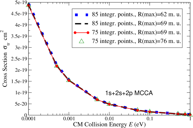
Figure 4: Numerical convergence results for the low-energy proton transfer reaction integral cross section $\sigma_{tr}$ in $\bar{\rm{p}}+\rm{H}_{\mu}\rightarrow(\bar{\rm{p}}\rm{p})_{\alpha}+\mu^{-}$, where $\rm{H}_{\mu}$ is a muonic hydrogen atom and $\alpha=$1s. In these calculations the polarization effects are included, i.e. the $1s+2s+2p$ MCCA approach is used.

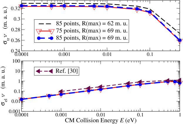
Figure 5: Upper plot: numerical convergence results for the low-energy proton transfer reaction integral cross section $\sigma_{tr}$ multiplied by the collision velocity v $=v_{c.m.}$. Lower plot: elastic scattering cross section $\sigma_{el}$ multiplied by the collision velocity v in $\bar{\rm{p}}+\rm{H}_{\mu}\rightarrow(\bar{\rm{p}}\rm{p})_{\alpha}+\mu^{-}$, where $\rm{H}_{\mu}$ is a muonic hydrogen atom and $\alpha=$1s. In these calculations only the $1s+2s+2p$ MCCA approach is used. Corresponding results (triangles left) from paper igarashi2008 are also shown in this figure.

Figs. 4 and 5 represent the convergence results in the framework of the $1s+2s+2p$ MCCA approach in which we solve six coupled integral-differential equations. In these cases we used a different number of integration points, namely 75 and 85 per the muonic radius length and also varied the values of the upper limit of the integration to 62, 69 and 76 m. a. u. Thus, the maximum number of integration knots used in this work is $N_{max}=76\times 85=6460$. It is seen that the results are in a good agreement with each other in regard to the transfer and the elastic cross sections. Thus, numerical convergence has been achieved.

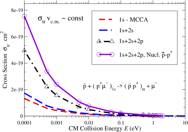
Figure 6: This figure shows our final result (after test calculations) for the low-energy proton transfer reaction integral cross section $\sigma_{tr}$ in the three-charge-particle collision $\bar{\rm{p}}+\rm{H}_{\mu}\rightarrow(\bar{\rm{p}}\rm{p})_{\alpha}+\mu^{-}$, where $\rm{H}_{\mu}$ is a muonic hydrogen atom: a bound state of a proton and a negative muon. Here only the reaction’s final channel with $\alpha$=1s in considered in the framework of the 1s, 1s+2s and 1s+2s+2p MCCA approach. The solid line with open circles is the result with an approximate inclusion of the strong $\bar{\rm{p}}$-$\rm{p}^{+}$ nuclear interaction.

We compared some of our findings with the corresponding data from the older work igarashi2008 . The $Pn$ formation cross section in the reaction (2) are shown in Fig. 6. Here we use $1s$, $1s+2s$ and $1s+2s+2p$ states within the modified close-coupling approximation, i.e. MCCA approach. One can see that the contribution of the $2s$- and $2p$-states from each target is becoming even more significant while the collision energy becomes smaller. It is useful to make a comment about the behavior of $\sigma_{tr}(\varepsilon_{coll})$ at very low collision energies: $\varepsilon_{coll}\sim 0$. From our calculations we found the following relationship in the p transfer cross sections: $\sigma_{tr}\rightarrow\infty$ as $\varepsilon_{coll}\rightarrow 0$. However, the p transfer rates, $\lambda_{tr}$, are proportional to the product $\sigma_{tr}v_{c.m.}$ and this trends to a finite value as $v_{c.m.}\rightarrow 0$.

To compute the proton transfer rate the following formula $\lambda_{tr}=\sigma_{tr}(\varepsilon_{coll}\rightarrow 0)v_{c.m.}$ can be used. Therefore, additionally, for process (2) we can compute the numerical value of the following important quantity:

$$\Lambda(Pn)=\sigma_{tr}(\varepsilon_{coll}\rightarrow 0)v_{c.m.}\approx\mbox{const},$$ (33)

which is proportional to the actual $Pn$ formation rate at low collision energies. In the framework of the 2$\times(1s+2s+2p)$ MCCA approach, i.e. when six coupled Faddeev-Hahn-type integral-differential equations are solved, our result for the $Pn$ formation rate has the following value:

$$\Lambda_{1s2s2p}(Pn)\approx 0.32\ \mbox{m.a.u}.$$ (34)

The corresponding rate from work igarashi2008 is: $\Lambda^{\prime}(Pn)\approx 0.2$ m.a.u. Both of these results are in agreement with each other. For comparison purposes our original result for $\Lambda_{1s2s2p}(Pn)$ has been multiplied by a factor of ”$\times 5$” to match work igarashi2008 .

One of the main goals of this work is to investigate the effect of the $\bar{\rm p}$-p nuclear interaction on the rate of the reaction (2). In Fig. 6 we additionally provide our cross sections for (2) including the nuclear effect in the final $Pn$ state. One can see, that the contribution of the strong interaction becomes even more substantial when the collision energy becomes lower. Also, for a few selected energies Table 1 shows our results for the $Pn$ formation total cross sections and rates in the framework of different MCCA approximations. The unitarity relationship, i.e. Eq. (32), is checked. It is seen, that $\chi$ exhibits fairly constant values close to one. A few additional comments about the inclusion of the $\bar{\rm p}$-p nuclear interaction are appropriate. First of all, we neglected the $\bar{\mbox{p}}$+p annihilation channel. This approximation has been discussed above. However, the effect of the strong nuclear forces on the reaction (2) is incorporated through the energy shifts $\Delta E_{n^{\prime}}^{\bar{N}N}$ to the original Coulomb energy levels in the $Pn$ atom, i.e. $\varepsilon_{n^{\prime}}$ in Eq. (20). To compute $\Delta E_{n^{\prime}}^{\bar{N}N}$ the expression (22) is used from deser . The $\bar{\mbox{p}}+$p elastic scattering length, i.e parameter $a_{s}$, was adopted from work jmr1992 and equals 0.57 fm in our calculations. In jmr1992 the Kohno-Weise strong interaction potential KW1986 has been applied.

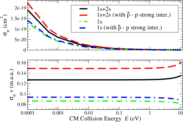
Figure 7: Upper plot: integral cross sections $\sigma_{tr}$ in the reaction (2) with and without inclusion of the $\bar{\rm{p}}$-p strong interaction. Only the $1s$ and $1s+2s$ approximations are used. Lower plot: corresponding results as on the top plot, but for the low-energy reaction rate: $\sigma_{tr}$ multiplied by the collision velocity v $=v_{c.m.}$.

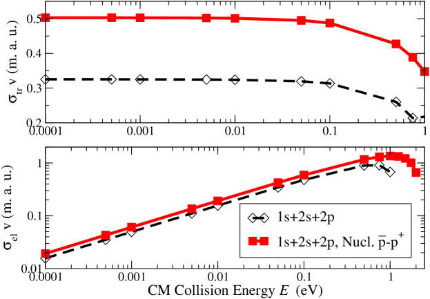
Figure 8: Upper plot: the reaction rate, i.e. integral cross sections $\sigma_{tr}$ of the reaction (2) multiplied by the collision velocity v with and without inclusion of the $\bar{\rm{p}}$-p strong interaction for comparison purposes. Only the $1s+2s+2p$ MCCA method is used in these calculations. Lower plot: corresponding results as on the top plot, but for the elastic scattering cross section of the process (2), $\sigma_{el}$, multiplied by the collision velocity v $=v_{c.m.}$.

The next two Figs. 7 and 8 represent results in which we compare cross sections and rates computed with and without the inclusion of the strong potential within the different close-coupling approximation. Fig. 7 shows our results in the framework of the $1s$ and $1s+2s$ MCCA approaches. The results are numerically stable. It seen that the contribution of the strong nuclear interaction is higher in the case of the $1s+2s$ approximation. For example, in this case the rate of the reaction (2) is about 0.12 m.a.u., however with the inclusion of the nuclear interaction it becomes 0.15 m.a.u. The last figure in this paper, Fig. 8, represents our computational data in the $1s+2s+2p$ approach. The very important polarization effect is included. The inclusion of the nuclear interaction brings a significant change to the rate of the reaction (2). At very low collision energies around $10^{-4}-10^{-2}$ eV the rate is $\sim$0.5 m.a.u. It is important to restate that all calculations carried out in this work have been done for the ground-to-ground state of (2), i.e. $\alpha=1$.

IV Conclusion

In summation, the complexity of the few-body system and the method utilized necessitated that only the total orbital momentum $L=0$ be taken into account. However, the method was indeed adequate for the slow and ultraslow collisions discussed previously. Further, it is important to note that the devised few-body equations (8)-(9) do exactly satisfy the Schrődinger equation. In cases in which the energies below the three-body break-up threshold occur this methodology provides advantages similar to the Faddeev equations fadd93 . This is because these equations are formulated to include wave function components which contain the correct physical asymptotes. The solution of these equations begins by using a close-coupling approach. This then leads to an expansion of the system’s wave function components into eigenfunctions of the subsystem (target) Hamiltonians, which results in a set of one-dimensional integral-differential equations upon completion of the partial-wave projection.

In an effort to expand the scope of the results a strong proton-antiproton interaction was included by appropriately shifting the Coulomb energy levels of the $Pn$ atom jmr1982 ; deser . Interestingly, this process increased the magnitude of the resulting values of the reaction cross section and corresponding rate by $\sim 50$%. Therefore, one further three-body reaction similar to (2) can also be of a sufficient future interest:

$$\bar{\mbox{p}}+{{}^{2}}\mbox{H}_{\mu}(1s)\rightarrow(\bar{\mbox{p}}\mbox{d})_{\alpha}+\mu^{-},$$ (35)

where ²H=d is the deuterium nucleus, $\mu^{-}$ and $\bar{\mbox{p}}$ are muon and antiproton respectively. This is because of a possible effect of the isotopic few-body quantum dynamic differences between reactions (2) and (35), and the nuclear interaction differences between $\bar{\mbox{p}}$ and p and $\bar{\mbox{p}}$ and d. In the future, it would be very interesting to compare the cross sections of both reactions.

Based on the results herein it seems logical for future work to include in Eqs. (14) the higher atomic target states such as $3s+3p+3d+4s+4p...$ as well as the continuum spectrum. Calculations of this type would be very interesting but challenging. The challenge is because at very low energy collisions the higher energy channels are closed and there is a significant energy gap between the states and the actual collision energies. Despite this limitation the primary contribution from s- and p-states (polarization) is still evaluated. In closing, the authors feel that including the strong $\bar{\rm p}$-p interaction explicitly in the numerical solution of Eqs. (10)-(11) could also provide an interesting and challenging direction for future theoretical research in this area.

*

Appendix A Numerical method and solutions

The delicacy of the three-charge-particle system consideration consists in the fact that the Coulomb potential is a singular function. This singularity is a major problem in numerical calculations involving few-body systems with Coulomb potentials. Below we provide a brief discussion of our numerical approach used in this paper. It would be somewhat simpler to reach a numerical solution for the set of coupled Eqs. (23) if only the most important -s and -p waves are included within the expansions (14), (17) and (19), and limit $n$ up to $n=2$ in the Eq. (14). This process results in a truncated set of six coupled integral-differential equations because in $\Psi_{1(2)}$ only 1s, 2s and 2p target two-body atomic wave-functions are included. This method could be considered as a modified version of the close coupling approximation containing six expansion functions. The resulting set of truncated integral-differential Eqs. (23) may be solved by using a discretization procedure. Specifically, on the right side of the equations the integrals over $\rho_{1}$ and $\rho_{2}$ can be replaced with sums using the trapezoidal rule abram . Further, the second order partial derivatives on the left side can be discretized by using a three-point rule abram . This process allows us to obtain a set of linear equations for the unknown coefficients $f^{(i)}_{\alpha}(k)$ ($k=1,N_{p}$) my2013 ; my03 . Then it is possible to ascertain through the symbolic-operator notations that the set of linear equations has the following characteristics my2013 ; my03 :

$$\sum_{\alpha^{\prime}=1}^{2\times N_{s}}\sum_{j=1}^{N_{p}}{\bf A}_{\alpha\alpha^{\prime}}(i,j)\vec{f}_{\alpha^{\prime}}(j)=\vec{b}_{\alpha}(i).$$ (36)

The resulting discretized equations can be then solved using the Gauss elimination method forsythe . It then follows that the matrix $\bf A$ should exhibit a well known block-structure. In this case there are four major blocks in the matrix: two of them are related to the differential operators and other two are related to the integral operators my2013 ; my03 . Further, each block should contain sub-blocks. The number of sub-blocks, of course, depends on the quantum numbers $\alpha=nl\lambda$ and $\alpha^{\prime}=n^{\prime}l^{\prime}\lambda^{\prime}$. It is worth noting that the second order differential operators produce three-diagonal sub-matrixes my03 .

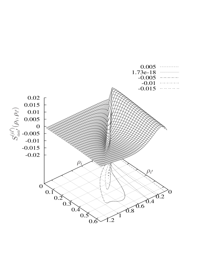
Figure 9: The two-dimensional function Eq. (A) (three-body angular integral), i.e. $S_{\alpha\alpha^{\prime}}^{ii^{\prime}}(\rho_{i},\rho_{i^{\prime}})$, when $\alpha=\alpha^{\prime}$=1s. The values of the coordinates $\{\rho_{i},\rho_{i^{\prime}}\}$ and the surface $S_{\alpha\alpha^{\prime}}^{ii^{\prime}}(\rho_{i},\rho_{i^{\prime}})$ are given in atomic muonic units.

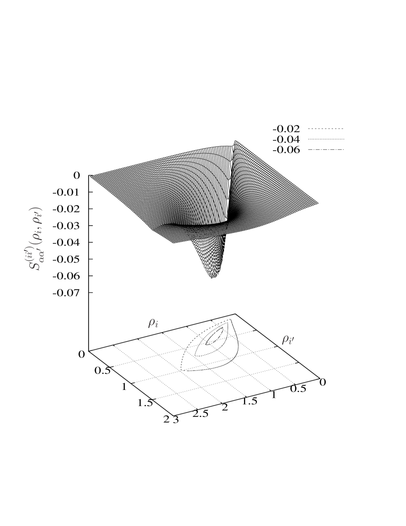
Figure 10: The two-dimensional function Eq. (A) (three-body angular integral), i.e. $S_{\alpha\alpha^{\prime}}^{ii^{\prime}}(\rho_{j},\rho_{k})$, when $\alpha$=1s and $\alpha^{\prime}$=2p. The values of the coordinates $\{\rho_{i},\rho_{i^{\prime}}\}$ and the surface $S_{\alpha\alpha^{\prime}}^{ii^{\prime}}(\rho_{i},\rho_{i^{\prime}})$ are given in atomic muonic units.

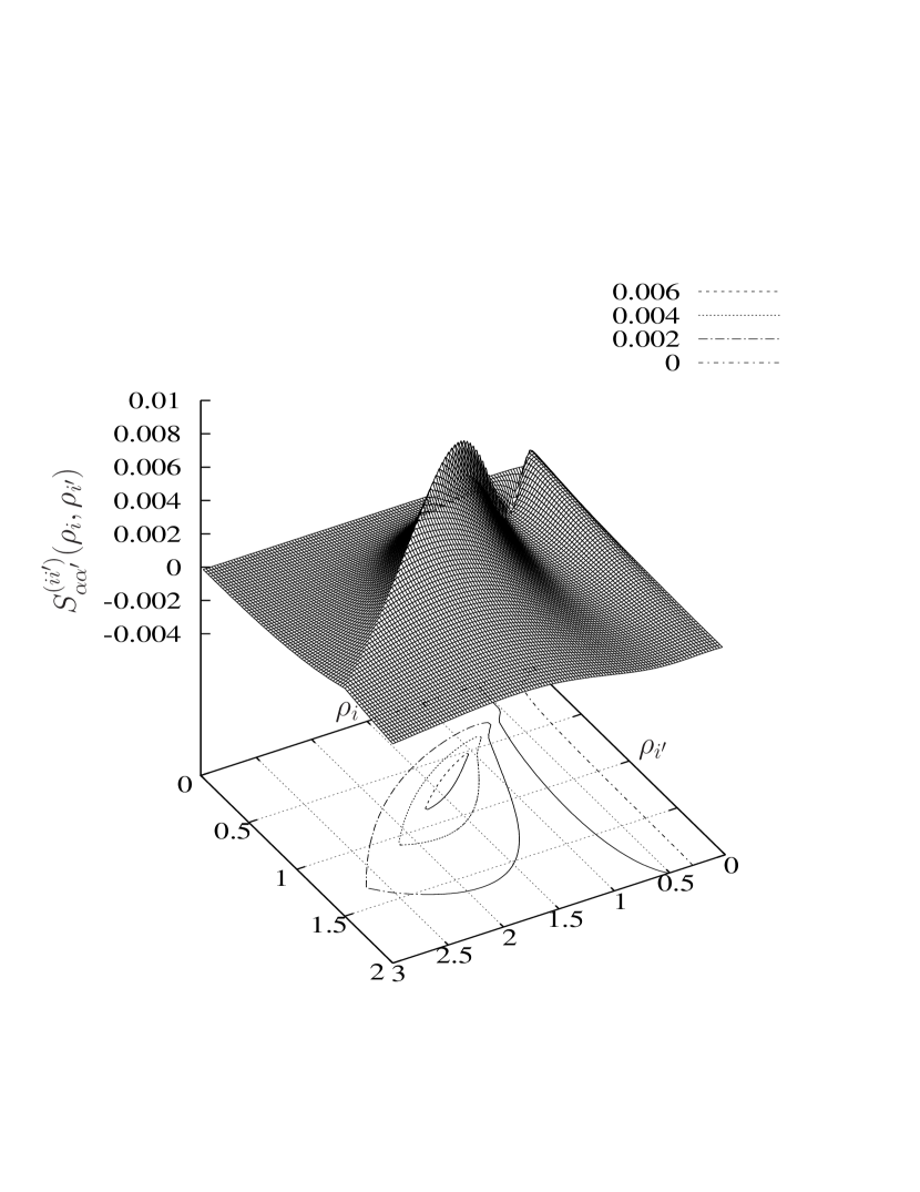
Figure 11: The two-dimensional function Eq. (A) (three-body angular integral), i.e. $S_{\alpha\alpha^{\prime}}^{ii^{\prime}}(\rho_{j},\rho_{k})$, when $\alpha=\alpha^{\prime}$=2s. The values of the coordinates $\{\rho_{i},\rho_{i^{\prime}}\}$ and the surface $S_{\alpha\alpha^{\prime}}^{ii^{\prime}}(\rho_{i},\rho_{i^{\prime}})$ are given in atomic muonic units.

The solution to the coupled integral-differential equations (23) requires one to first compute the angular integrals $S_{\alpha\alpha^{\prime}}^{(ii^{\prime})}(\rho_{i},\rho_{i^{\prime}})$ $(i\neq i^{\prime}=1,2)$ my2013 . These integrals are independent of the energy, $E$. To improve efficiency, one can compute them only once and then store them on a computer’s hard drive for future reference. For example, they could be used in the calculations required to determine charge-transfer cross-sections at different collision energies. Also noteworthy is the relationship of the sub-integral expressions which have a very strong and complicated dependence on the Jacobi coordinates $\rho_{i}$ and $\rho_{i^{\prime}}$ my2013 . The next three figures presented 9, 10 and 11 depict some of these relationships using different quantum numbers $\alpha$ and $\alpha^{\prime}$. Specifically, Fig. 9 depicts the result in a case where $\alpha=\alpha^{\prime}=1s$. In other words, this case illustrates a crucial ground-state to ground-state matrix element in Eqs. (23) within the input channel. Further evaluation reveals that this surface has smaller numerical values relative to the matrix element shown in Fig. 10. In this case $\alpha=1s$ and $\alpha^{\prime}=2p$, which assumes that the polarization effect is taken into account. An interesting case when $\alpha=\alpha^{\prime}=2s$ in the input channel is shown in Fig. 11. Further, the analysis reveals that a very strong polarization effect results in the input channel of the reaction (2). To clarify this further, one can calculate $S_{\alpha\alpha^{\prime}}^{(ii^{\prime})}(\rho_{i},\rho_{i^{\prime}})$ at different values of $\rho_{i}$ and $\rho_{i^{\prime}}$. To do this an adaptable algorithm has been devised and applied using the following mathematical substitution my2013 : $\cos\omega=(x^{2}-\beta_{i}^{2}\rho_{i}^{2}-\rho_{i^{\prime}}^{2})/(2\beta_{i}\rho_{i}\rho_{i^{\prime}}).$ The angle dependent portion of the resulting equation can be described by the following one-dimensional integral:

$$S_{\alpha\alpha^{\prime}}^{(ii^{\prime})}(\rho_{i},\rho_{i^{\prime}})=\frac{4\pi}{\beta_{i}}\frac{[(2\lambda+1)(2\lambda^{\prime}+1)]^{\frac{1}{2}}}{2L+1}\int_{|\beta_{i}\rho_{i}-\rho_{i^{\prime}}|}^{\beta_{i}\rho_{i}+\rho_{i^{\prime}}}dxR_{nl}^{(i)}(x)\left[-1+\frac{x}{r_{ii^{\prime}}(x)}\right]R_{n^{\prime}l^{\prime}}^{(i^{\prime})}(r_{i3}(x))$$

$$\times\sum_{mm^{\prime}}D_{mm^{\prime}}^{L}(0,\omega(x),0)C_{\lambda 0lm}^{Lm}C_{\lambda^{\prime}0l^{\prime}m^{\prime}}^{Lm^{\prime}}Y_{lm}(\nu_{i}(x),\pi)Y^{*}_{l^{\prime}m^{\prime}}(\nu_{i^{\prime}}(x),\pi).\ \$$ (37)

Specifically, the adaptive algorithm incorporated in a FORTRAN subroutine from berlizov99 is used within this work to calculate the angle integration in (A). This recursive computer program known as QUADREC, is an improved version of the well respected program QUANC8 forsythe . Therefore, QUADREC can provide improvements in regard to quality, stability and precision in integration when compared to QUANC8 berlizov99 . When considering the expression (A) it is worth noting that it differs from zero only in a quite narrow strip, i.e. when $\rho_{i}\approx\rho_{i^{\prime}}$. This can be explained because in the three-body system considered the coefficient $\beta_{i}$ approximately equals one. This means to it is imperative, to distribute a very large number of discretization points (up to 6000) between 0 and $\sim$80 muonic units if numerically reliable converged results are to be reached.

We mentioned above, that the truncated set of coupled integral-differential equations (23) is solved with the use of the matrix approach. The computation itself is organized in the following way: as a first step two sets of integration knots are created over the Jacobi coordinates $\rho_{1}$ and $\rho_{2}$, i.e. we have: $\{\rho_{1i},i=1,N_{1}\}$ and $\{\rho_{2j},j=1,N_{2}\}$. We choose $N_{1}=N_{2}=N$, where $N$ is taken up to 6500 points. Within the second step of the method we have to carry out a numerical computation of the angle integrals (A) for each given coordinate value: $\rho_{1i}$ and $\rho_{2j}$. A special FORTRAN adaptive-quadrature subroutine is used in this work. Because of the very singular character of the Coulomb pair-interaction potentials between the particles this step is important but very challenging and time consuming. Based on our observation, the precision and quality of these calculations should be robust enough. The calculated angle integrals, Eq. (A) can be saved on a hard drive of a computer system. After this initial, but very important work our program builds the full matrix which precisely corresponds to the set of coupled Eqs. (23). Finally, one can solve the set of the linear equations (36), compute the three-body wave function, the elastic and charge-transfer cross sections, and the corresponding $Pn$ formation rates.

Also, it would be useful to make few additional comments about the structure of the Eqs. (23) and our numerical method. Namely, on the left side of these equations we have the usual differential operators. However, because coupled Faddeev-Hahn-type equations are used in this work, on the right side of the equations Eqs. (23) we have the unknown functions under the integration over $\rho_{1}$ and $\rho_{2}$. The integration runs from 0 to infinity. Therefore, it is obvious, that the usual step-by-step or predictor-corrector numerical methods in which a computer program itself (automatically) adopts integration steps forsythe cannot be applied in these calculations. Consequently, in the current case one needs, first, to choose and distribute the integration knots in accord with the peculiarities of the potential surfaces (A) and then build the full matrix. In turn the surfaces (matrix elements) $S_{\alpha\alpha^{\prime}}^{(ii^{\prime})}(\rho_{i},\rho_{i^{\prime}})$ have quite complicated and very different shapes and values. This is seen in Figs. 9, 10, and 11. It is very important not to lose all these peculiarities and carefully distribute as well as utilize a large number of integration points. However, the last circumstance results in a very large matrix.

Another complication arises from the fact that the reaction (2) in the input channel has a muonic atom H_μ as a target, but in the output channel $Pn$ is present. The size of $Pn$ is about five times smaller than H_μ, therefore the number of the integration knots which are sufficient to describe the H_μ channel may not be good enough to compute the $Pn$ channel.

Table 1: The total $Pn$ formation cross sections $\sigma_{tr}(\varepsilon_{coll})$ and rates $\Lambda(Pn)$ in the three-body reaction (2), when $\alpha=1$ and $\varepsilon_{coll}$ is the collision energy. The results are presented in the framework of the different MCCA approach: $1s$, $1s+2s$, and $1s+2s+2p$. The cross section $\sigma_{tr}$ is given in cm² and $\Lambda(Pn)$ in m.a.u. The unitarity condition coefficient $\chi$, i.e. Eq. (32), is also shown. Results with the inclusion of the strong nuclear interaction between $\bar{\mbox{p}}$ and p are presented only in the $1s+2s+2p$ approximation. For convenience, rates $\Lambda$’s have been multiplied by factor of ”$\times 5$” in this table, as in Ref. igarashi2008 . The rate with inclusion of the nuclear interaction, i.e. $\Lambda^{\bar{\rm{p}}\rm{p}}$, is also multiplied by the same factor.

	$1s$		$1s+2s$			$1s+2s+2p$		$1s+2s+2p$, Nucl. $\bar{\rm{p}}$-$\rm{p}$
$\varepsilon_{coll}$	$\sigma_{tr}$	$\Lambda(Pn)$	$\sigma_{tr}$	$\Lambda(Pn)$	$\chi$	$\sigma_{tr}$	$\Lambda(Pn)$	$\sigma^{\bar{\rm{p}}\rm{p}}_{tr}$	$\Lambda^{\bar{\rm{p}}\rm{p}}(Pn)$
0.0001	1.3E-19	0.08639	1.9E-19	0.1269	0.97	4.95E-19	0.3251	7.55E-19	0.5027
0.001	4.1E-20	0.08639	6.0E-20	0.1269	0.98	1.57E-19	0.3249	2.39E-19	0.5025
0.05	5.8E-21	0.08636	8.5E-21	0.1269	0.97	2.18E-20	0.3193	3.33E-20	0.4950
1.0	1.3E-21	0.08593	1.9E-21	0.1273	0.97	2.89E-21	-	5.22E-21	-
10.0	3.9E-22	0.08183	6.4E-22	0.1343	0.97		-	-	-

References

- (1) O. Chamberlain, E. Segr, C. Wiegand, and T. Ypsilantis Phys. Rev. 100, 947 (1955).
- (2) G. B. Andresen et al., (ALPHA Collaboration), Phys. Rev. Lett. 105 013003 (2010).
- (3) G. Gabrielse et al., (ATRAP Collaboration), Phys. Rev. Lett. 106 073002 (2011).
- (4) M. Hori and J. Waltz, Prog. Part. Nucl. Phys. 72, 206 (2013).
- (5) M. Amoretti et al., Nature 419, 6906 (2002).
- (6) M. Ahmadi et al. Nature http://dx.doi.org/10.1038/nature21040 (2016).
- (7) V. A. Kosteleck and A. J. Vargas, Phys. Rev. D 92, 056002 (2015).
- (8) W. A. Bertsche, E. Butler, M. Charlton, and N. Madsen, J. Phys. B: At. Mol. Opt. Phys. 48, 232001 (2015).
- (9) R. S. Hayano, M. Hori, D. Horvath, and E. Widmann, Rep. Prog. Phys. 70, 1995 (2007).
- (10) M. Hori et al., Nature 475, 484 (2011).
- (11) N. Zurlo et al., (ATHENA Collaboration), Phys. Rev. Lett. 97, 153401 (2006); Hyperfine Interact. 172, 97 (2006).
- (12) L. Venturelli et al., Nucl. Instrum. Methods Phys. Res., Sect. B 261, 40 (2007).
- (13) E. L. Rizzini et al., Europ. Phys. J. Plus, 127, 1 (2012).
- (14) I. S. Shapiro, Phys. Rep. 35, 129 (1978).
- (15) J. Hrtnkov and J. Mare, Nucl. Phys. A 945, 197 (2015).
- (16) J. Carbonell. J. -M. Richard, and S. Wycech, Z. Phys. A 343, 325 (1992).
- (17) C. B. Dover and J. -M. Richard, Phys. Rev. C 25, 1952 (1982).
- (18) J. -M. Richard and M. E. Sainio, Phys. Lett. B 110, 349 (1982).
- (19) B. R. Desai, Phys. Rev. 119, 1385 (1961).
- (20) E. Klempt, F. Bradamante, A. Martin, J.-M. Richard, Phys. Rep. 368, 119 (2002).
- (21) E. Klempt, C. Batty, J.-M. Richard, Phys. Rep. 413, 197 (2005).
- (22) L. N. Bogdanova, O. D. Dalkarov, and I. S. Shapiro, Ann. Phys. 84, 261 (1974).
- (23) X. M. Tong, K. Hino, N. Toshima, Phys. Rev. Lett. 97, 243202 (2006).
- (24) K. Sakimoto, Phys. Rev. A 88 012507 (2013).
- (25) B. D. Esry and H. R. Sadeghpour, Phys. Rev. A 67, 012704 (2003).
- (26) M. Born and R. Oppenheimer, Ann. Phys., Liepzig, 84, 457 (1927).
- (27) T. Ueda, Prog. Theor. Phys. 62, 1670 (1979.)
- (28) B. Lauss, Nucl. Phys. A 827, 401c (2009).
- (29) L. D. Faddeev, Zh. Eksp. Teor. Fiz. 39 1459 (1960) [Sov. Phys. JETP 12 1014 (1961)].
- (30) L. D. Faddeev and S. P. Merkuriev, Quantum Scattering Theory for Several Particle Systems, (Kluwers Academic Publishers, Dordrecht, 1993); L. D. Faddeev, Mathematical Aspects of the Three-Body Problem in the Quantum Scattering Theory, (Israel, Program for Scientific Translation, Jerusalem, 1965).
- (31) A. Igarashi and N. Toshima, Eur. Phys. J. D 46, 425 (2008).
- (32) Y. Hahn and K. Watson, Phys. Rev. A 5 1718 (1972); Y. Hahn, Nucl. Phys. A 389, 1 (1982).
- (33) R. A. Sultanov and S. K. Adhikari, Phys. Rev. A 61, 227111 (2000); A 62, 022509 (2000); R. A. Sultanov, Few-Body Syst. Suppl. 10, 281 (1999).
- (34) R. A. Sultanov, D. Guster, and S. K. Adhikari, Few-Body Syst. 56, 793 (2015).
- (35) R. A. Sultanov and D. Guster, J. Comp. Phys. 192, 231 (2003); J. Phys. B: At. Mol. Opt. Phys. 46 215204 (2013); EPJ Web of Conf. 122, 09004 (2016).
- (36) S. P. Merkuriev, Ann. Phys. 130, 395 (1980).
- (37) L. D. Landau and E. M. Lifshitz, Quantum Mechanics, Non-Relativistic Theory, Third Edition, Course of Theoretical Physics, Volume 3, (Butterworth-Heinemann, 2003).
- (38) S. Deser, M. L. Goldberger, K. Baumann, and W. Thirring, Phys. Rev. 96, 774 (1954).
- (39) D. A. Varshalovich, A. N. Moskalev, and V. L. Khersonskii, Quantum Theory of Angular Momentum, (World Scientific, Singapore, 1988).
- (40) E. A. G. Armour, Y. Liu, and A. Vigier, J. Phys. B: At. Mol. Opt. Phys. 38, L47 (2005).
- (41) T. L. Trueman, Nucl. Phys. 26, 57 (1961).
- (42) V. S. Popov, A. E. Kudryavtsev, and V. D. Mur, Sov. Phys. JETP 50 (5), 865 (1979).
- (43) J. Thaler, J. Phys. G: Nucl. Phys. 9, 1009 (1983); 11, 201 (1985).
- (44) A. Adamczak, C. Chiccoli, V. I. Korobov, V. S. Melezhik, P. Pasini, L. I. Ponomarev, and J. Wozniak, Phys. Lett. B 285, 319 (1992).
- (45) J.S. Cohen and M.C. Struensee, Phys. Rev. A 43, 3460 (1991).
- (46) A. A. Kvitsinsky, J. Carbonell, C. Gignoux, Phys. Rev. A 51, 2997 (1995).
- (47) G. E. Forsythe, M. A. Malcolm, and C. B. Moler, Computer Methods in Mathematical Computations, (Prentice-Hall, Inc., Englewood Cliffs, New Jersey 1977).
- (48) M. Kohno and W. Weise, Nucl. Phys. A 454, 429 (1986).
- (49) M. Abramowitz and I. A. Stegun, Handbook of Mathematical Functions: with Formulas, Graphs, and Mathematical Tables, (Dover Publications, New York, 1965).
- (50) A. N. Berlizov and A. A. Zhmudsky, arXiv:physics/9905035v2.
TABLE I and FIGURES 111